Abstract

We discuss the near singularity region of the linear mass Vaidya metric for massless particles with non-zero angular momentum. In particular we look at massless geodesics with non-zero angular momentum near the vanishing point of a special subclass of linear mass Vaidya metrics. We also investigate this same structure in the numerical solutions for the scattering of massless scalars from the singularity. Finally we make some comments on the possibility of using this metric as a semi-classical model for the end-point of black hole evaporation.

1 Introduction

The linear mass Vaidya metric is a special class of Vaidya metrics [1, 2, 3] over which one has a certain degree of analytic control, in particular as a consequence of the additional homothety symmetry that these metrics possess. In general the Vaidya metric has the form

$$\mathrm{d}s^{2}=-\left(1-\frac{2m(u)}{r}\right)\mathrm{d}u^{2}-2\,\mathrm{d}u\,\mathrm{d}r+r^{2}\mathrm{d}\Omega^{2}$$ (1.1)

and when $m(u)=-\mu u$ this metric has a homothety symmetry under rescaling of the coordinates $u$ and $r$ together with an overall rescaling of the metric. In addition, when $0<\mu<1/16$ these metrics have the special property that they contain a null singularity that vanishes at an interior point of the spacetime. These metrics have been studied in detail in [4] and for the above range of $\mu$ the detailed causal structure of the space-time is illustrated in the Penrose diagram of figure (1) where $\mathcal{D}$ indicates the vanishing point. These metrics have been used in [5, 6, 7, 8, 9, 10, 11, 12, 13, 14, 15, 16, 17] to study various aspects of black hole evaporation and cosmic censorship. Nevertheless there is still no consistent picture of the complete evaporation of a black hole. The current paper does not claim to resolve this question but presents various arguments to support the proposal that the final stages of evaporation can be modelled at the semi-classical level by a linear mass Vaidya metric.

The outgoing Vaidya metric has also recently been used in [18] to study evaporating black-holes and unitarity. Questions of information loss and unitarity are of great interest but the current paper does not address them as we are specifically looking at the evolution from the Page time [19] (the time after which, assuming that evaporation is unitary, a black hole has reemitted almost all of the information that it contained), up to its complete evaporation.

The motivation for this paper is to propose these linear-mass Vaidya metrics as semi-classical models for the end-point of black hole evaporation. To make this more realistic, one should use a more general mass function that follows the Hawking radiation formula $m(u)=(-u)^{1/3}$ up to the point that the mass of the black hole becomes Planckian, after which it becomes linear. It is generally hypothesised that black hole evaporation concludes with the complete disappearance of the black hole and the singularity that it contains. We do not know precisely what happens beyond the future horizon of this (possibly cataclysmic) event but one expects that the space-time returns to an asymptotically flat and non-singular configuration (protected from more singular fates by cosmic censorship and positive mass theorems). We will assume that the linear mass Vaidya metric is continuously attached to Minkowski space-time as in [20] (some discussion of these issues in a slightly more general context can also be found in [21]). A qualitative sketch of this evolution is illustrated in figure (2).

Figure 1: Penrose diagram for the linear mass Vaidya metric with $0<\mu<1/16$, $\mathcal{D}$ is the vanishing point.

To investigate the viability of this picture in this paper we perform a detailed study of null geodesics and massless scalar fields with non-zero angular momentum in the linear mass Vaidya metrics. We will use a mixture of analytic and numerical techniques to get a complete picture of their behaviour. Our aim is to demonstrate that, close to the vanishing point, the null-singularity effectively becomes repulsive and consequently stable under the effects of small perturbations, backscattering and subsequent backreaction. This stability is a necessary condition for the suitability of this metric as a semi-classical model for the end-point of black hole evaporation.

Most of this article is dedicated to the presentation and discussion of the analysis for massless particles with non-zero angular momentum. In the first section we will look at null ingoing geodesics and then in the second section we study the wave-equation for a massless scalar in this background. In the concluding section we will present a discussion of our results and some additional evidence for our proposal that the linear mass Vaidya metric is a viable candidate for a semi-classical model of the final stages of black hole evaporation.

2 Null geodesics

In the following we will be investigating particles in the background of the linear mass Vaidya metric with $m(u)=-\mu u$ studied in detail by Waugh and Kayll Lake [4]

$$\mathrm{d}s^{2}=-\left(1+\frac{2\mu u}{r}\right)\mathrm{d}u^{2}-2\,\mathrm{d}u\,\mathrm{d}r+r^{2}\mathrm{d}\Omega^{2}.$$ (2.1)

Figure 2: An adiabatically evaporating Schwarzschild space-time evolving to a linear mass Vaidya metric. $\mathcal{D}$ is the vanishing point and $\mathcal{SH}$ the stretched horizon. The region $\mathcal{S}$ is blown up in figure(6).

For $0<\mu<1/16$ this class of space-times has the conformal structure illustrated in figure (1) – note in particular that to the future of the vanishing point $\mathcal{D}$ there is no longer a singularity. This metric (for $u<0$) is a solution to the Einstein equations with the stress-energy tensor

$$T_{\alpha\beta}=\frac{\mu}{4\pi Gr^{2}}\delta_{\alpha}^{u}\delta_{\beta}^{u}$$ (2.2)

corresponding to a purely out-going spherically symmetric flux of radiation.

We are interested in null geodesics with non-zero angular momentum in region II of figure 1. For zero angular momentum the null geodesic equations are integrable and one can find various discussions of these in the literature e.g. [5]. The above coordinate system is however not very useful for the study of the metric in particular near the null singularity due to the degeneracy between $r$ and $u$ for $u\rightarrow 0^{-}$. In fact, as the singularity is approached we find that away from the end-point $r\rightarrow-u(1-\Delta)/4$ while precisely at the end-point $r\rightarrow-u(1+\Delta)/4$, where $\Delta=\sqrt{1-16\mu}$. It will be convenient to sometimes also use the coordinate $z=-u/r$ in terms of which $r\rightarrow r_{\pm}=-u(1\pm\Delta)/4$, corresponding to $z\rightarrow z_{\mp}=(1\pm\sqrt{1-16\mu})/4\mu$ as indicated in figure (1). Note that region II corresponds to $r_{-}<r<r_{+}$ ($z_{+}>z>z_{-}$, as $z_{\pm}=-1/r_{\mp}$). To study the behaviour of the metric around the vanishing point ${\mathcal{D}}$ it is much more convenient to change to the double-null coordinates [4] for which the metric has the form

$$\mathrm{d}s^{2}=-2f(u,v)\,\mathrm{d}u\,\mathrm{d}v+r(u,v)^{2}\mathrm{d}\Omega^{2}$$ (2.3)

with source

$$T_{\alpha\beta}=\frac{\mu}{4\pi Gr(u,v)^{2}}\delta^{u}_{\alpha}\delta^{u}_{\beta}$$ (2.4)

and where

$$f(u,v)=\frac{1+\Delta}{2\Delta r(u,v)}\left(r(u,v)+u(1-\Delta)/4\right)^{2/(1+\Delta)}.$$ (2.5)

In these coordinates $v=0$ coincides with $r=r_{+}=-u(1+\Delta)/4$ ($z=z_{-}$) while the singularity is at $u=0$ and $v<0$ corresponding to $r=r_{-}=-u(1-\Delta)/4$ ($z=z_{+}$). The coordinate transformation from $(u,r)$ to $(u,v)$ can be obtained, in principle, by solving the implicit equation [4]

$$|v|^{1+\Delta}\left(r(u,v)+u(1-\Delta)/4\right)^{1-\Delta}=\left(r(u,v)+u(1+\Delta)/4\right)^{1+\Delta}$$ (2.6)

for $r(u,v)$. For the specific values $\Delta=1/5,1/3$ and $1/2$ where $\Delta=\sqrt{1-16\mu}$, $r(u,v)$ can be found explcitly by solving at most a cubic polynomial equation, leading to the following expressions for $r_{\Delta}(u,v)$;

$$r_{1/5}(u,v)= \frac{1}{30}\left(\sqrt[3]{5}v\left(\sqrt[3]{-\sqrt{27\left(u^{3}\left(27u-40v^{3}\right)\right)}+27u^{2}-180uv^{3}+200v^{6}}\right.\right.$$

$$+ \left.\left.\sqrt[3]{\sqrt{27\left(u^{3}\left(27u-40v^{3}\right)\right)}+27u^{2}-180uv^{3}+200v^{6}}\right)-9u+10v^{3}\right),$$ (2.7)

$$r_{1/3}(u,v)=\frac{1}{2}\left(v\sqrt{v^{2}-\frac{2u}{3}}-\frac{2u}{3}+v^{2}\right),$$ (2.8)

$$r_{1/2}(u,v)=\frac{1}{8}\left(\frac{4}{3^{2/3}}\left(\sqrt[3]{\sqrt{3v^{6}\left(27u^{2}-64v^{3}\right)}-9uv^{3}}+\sqrt[3]{\sqrt{3v^{6}\left(27u^{2}-64v^{3}\right)}+9uv^{3}}\right)-3u\right).$$ (2.9)

These explicit forms for $r(u,v)$ will be used for the quantitative numerical analysis of the geodesic equations and below also for the numerical study of a massless scalar field on this geometry.

Due to the spherical symmetry angular momentum $L$ is conserved and the null condition is

$$\frac{L^{2}}{r^{2}}=\left(1+\frac{2\mu u}{r}\right)\dot{u}^{2}+2\dot{u}\dot{r}=2f(u,v)\dot{u}\dot{v}.$$ (2.10)

In addition, the linear mass Vaidya metrics have a homothety symmetry under rescalings of $u$ and $r$ with a corresponding overall rescaling of the metric. This gives rise to an additional conserved quantity

$$P=\left(1+\frac{2\mu u}{r}\right)u\dot{u}+r\dot{u}+u\dot{r}$$ (2.11)

Solving these two equations for $\dot{u}$ and $\dot{v}$ we find

$$\dot{u}^{\pm}=P\frac{1\pm\sqrt{1-\frac{L^{2}}{P^{2}}\frac{u}{r}k(u/r)}}{rk(u/r)}$$ (2.12)

and

$$\dot{v}^{\pm}=\frac{L^{2}}{2fr^{2}\dot{u}^{\pm}},$$ (2.13)

where

$$k(u/r)=2\mu\frac{u^{2}}{r^{2}}+\frac{u}{r}+2.$$ (2.14)

In region II, between the two roots $r=r_{\pm}$ of $k(u/r)$ we demand that both $\dot{u}$ and $\dot{v}$ are positive (guaranteeing that the geodesics are future directed) and this leads to the requirement that $P<0$. This implies that to each value of $P<0$ there correspond two distinct solutions for $(\dot{u}^{\pm},\dot{v}^{\pm})$. They are both physical but correspond to two different ranges of initial conditions. We can qualitatively understand the behaviour of these solutions by considering the argument of the square root in the expression for $\dot{u}$. Clearly any complete classical trajectory (that does not run into the singularity) should be such that the argument of the square root is always positive, leading to the constraint that

$$h(z)=-z(2\mu z^{2}-z+2)\leq\frac{P^{2}}{L^{2}}.$$ (2.15)

The crossover from the $+$ branch solutions for $(\dot{u},\dot{v})$ to the $-$ branch solutions occurs at the trajectory $h(z)=P^{2}/L^{2}$. These special trajectories are indicated in figure (3) by the boundaries of the classically forbidden regions.

$h(z)$ has a maximum at $z=z_{\text{max}}$ between $z^{+}$ and $z^{-}$ along the curve

$$\frac{u}{r}=-z_{\text{max}}=-\frac{1}{6\mu}(1+\sqrt{1-12\mu})$$ (2.16)

and its value there is

$$h_{\text{max}}=\frac{(1+\sqrt{1-12\mu})(1+\sqrt{1-12\mu}-24\mu)}{108\mu^{2}}.$$ (2.17)

Ingoing particles with $z<z_{\text{max}}$ and $P^{2}/L^{2}<h_{\text{max}}$ will be reflected by the potential barrier continuing on to $\mathcal{I}^{+}$. Taking the limit of small $\mu$, one finds the bound $P^{2}/L^{2}<1/(27\mu^{2})$ which is the same as that for massless geodesics outside a Schwarzschild black hole of mass $\mu$. For particles with $P^{2}/L^{2}>h_{\text{max}}$ on the other hand, they clearly run into the singularity coming in from $z<z_{\text{max}}$. The numerical plots of the vector fields $(\dot{u}^{\pm},\dot{v}^{\pm})$ shown in figure (3) confirm this qualitative analysis. We will refer to the curve $z=z_{\text{max}}$ as the Vaiyda photon sphere. It plays exactly the same role as the photon sphere for the Schwarzschild metric which lies at $r=3GM$ and has a height $E^{2}/L^{2}=1/(27M^{2})$ – incoming/outgoing photons below the barrier will be reflected while those above the barrier continue in the same direction.

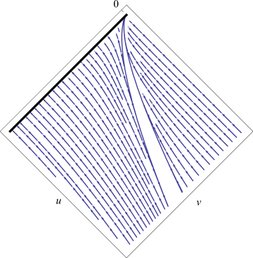
(a) $\dot{u}^{+}(u,v)$

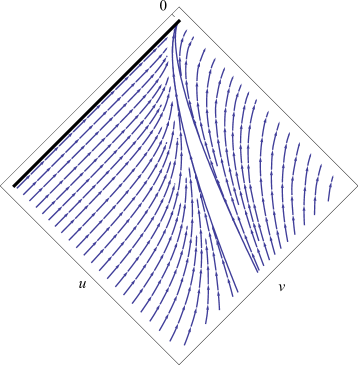
(b) $\dot{u}^{-}(u,v)$

Figure 3: Region II near the singularity for $\Delta=1/2$. The white region is classically forbidden when $P^{2}/L^{2}<h_{\text{max}}=3.75575$ and for the plot we chose $P^{2}/L^{2}=3.7$.

This above analysis gives us a clear picture of the qualitative behaviour of geodesics, however the full numerical analysis of these equations remains quite complicated. To confirm our qualitative discussion, we can extract some analytic information from the geodesic equations if we take a near singularity limit. In particular we can expand around small $v$, studying the behaviour as $u\rightarrow 0^{-}$. The ratio $\dot{u}/\dot{v}$ expanded for small $u$ and $v$

$$\frac{\mathrm{d}u}{\mathrm{d}v}=\frac{\dot{u}}{\dot{v}}=(-u)^{a}(-v)^{b}$$ (2.18)

is characterised by the exponents $a$ and $b$ with solution

$$u(v)=-\left(\frac{1-a}{1+b}(-v)^{1+b}+C\right)^{1/(1-a)}.$$ (2.19)

We can easily see that geodesics will avoid the singularity at $u=0$ and $v<0$ only if both $1-a$ and $1+b$ are negative. To determine the exponents we need an expansion of $r(u,v)$ around $u=0$. In the region $v<0$ and for $u\rightarrow 0^{-}$ one can solve to sub-leading order in $u$ the implicit equation (2.6) for $r_{\Delta}(u,v)$ giving

$$r_{\Delta}(u,v)=-\frac{u(1-\Delta)}{4}+\left(-\frac{\Delta u}{2v}\right)^{(1+\Delta)/(1-\Delta)}.$$ (2.20)

It is easy to check that for the $(u^{+},v^{+})$ branch $a=(1-3\Delta)/(1-\Delta)$ and $b=2\Delta/(1-\Delta)$, while for the $(u^{-},v^{-})$ branch we have $a=(1+\Delta)/(1-\Delta)$ and $b=-2/(1-\Delta)$. Thus for the $+$ branch there is a class of geodesics that can run into the singularity while for the $-$ branch the geodesics go precisely to the vanishing point at $u=v=0$. Alternatively we can look at an expansion relevant for geodesics approaching the potential barrier from the external region. The “$-$” branch is such that all geodesics cross the $v=0$ line before reaching $u=0$ while all of the $+$ branch solutions again go to the vanishing point at $u=v=0$. These conclusions clearly agree with the flow lines of the explicit solutions for $(\dot{u}^{\pm},\dot{v}^{\pm})$ displayed in figure (3).

3 Massless scalar field

To further understand the nature of the null singularity and the potential barrier that surrounds it we will now present the results of the numerical analysis of a massless scalar field in this geometry, in particular studying the scattering of an in-going gaussian wave packet from the near singularity region.

In double-null coordinates the wave-equation for a massless scalar field is

$$\frac{\partial^{2}\Psi}{\partial u\,\partial v}+\frac{\ell(\ell+1)}{2r^{2}}f\Psi=0.$$ (3.1)

The potential $V(u,v)$ is infinite around the vanishing point, and is also divergent along the null-singularity when $\Delta<1/3$ as can be seen clearly in figure (4). As can be seen from the plots the potential for $\Delta=1/2$ grows more rapidly in the region $v<0$ than does that for $\Delta=1/5$, the crossover between these two behaviours is at $\Delta=1/3$ (not shown) for which the potential is completely symmetric about $v=0$.

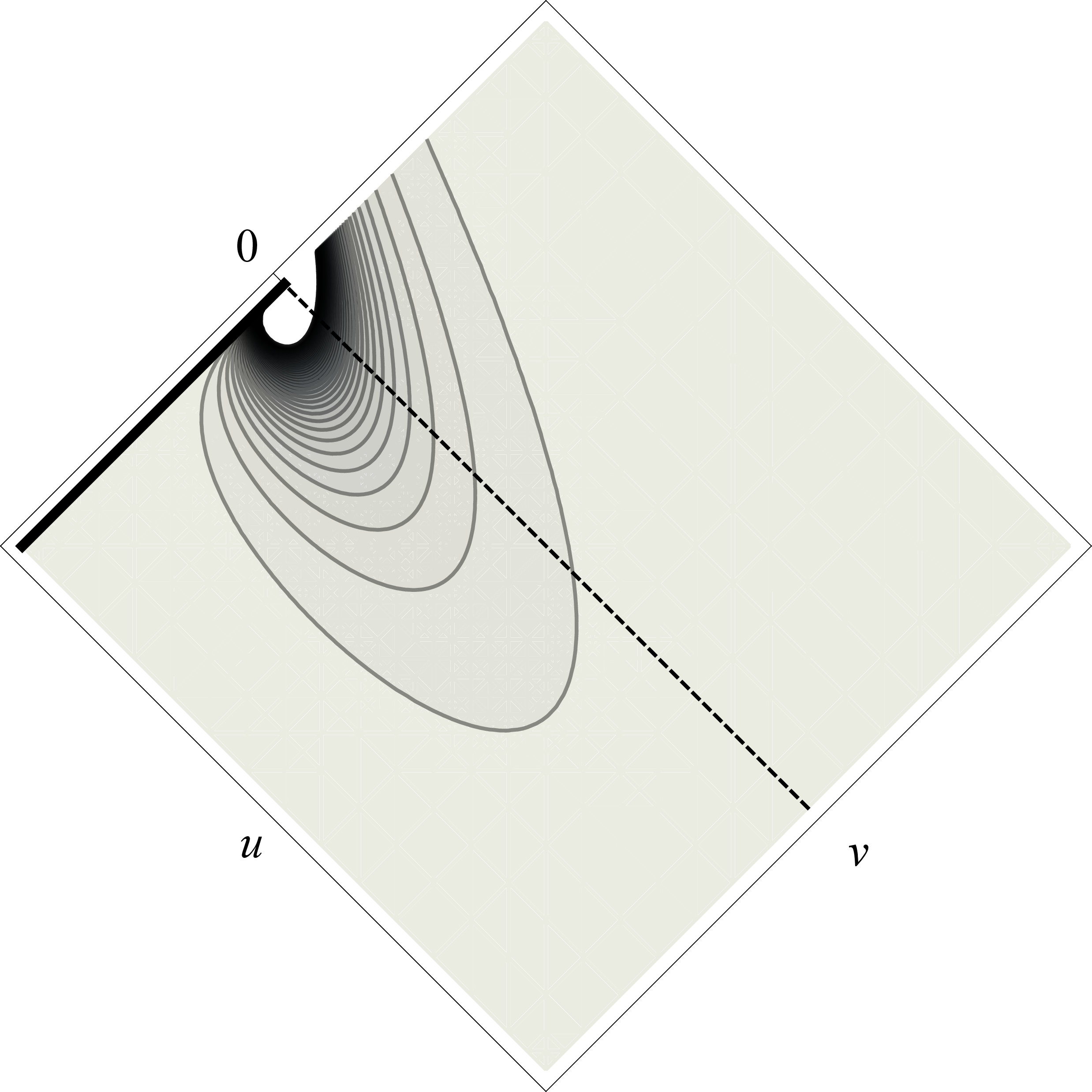
(a) $\Delta=1/2$

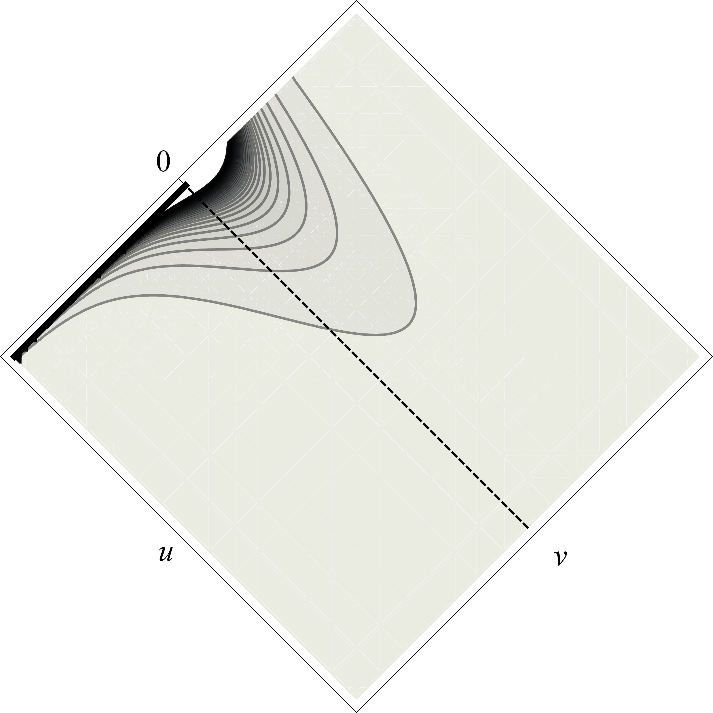
(b) $\Delta=1/5$

Figure 4: Scattering potentials on the boundary between regions II and III. Darker shades correspond to larger $V(u,v)$ with divergence precisely at $u=v=0$ for $\Delta=1/2$ and at $u=0$, $v<0$ for $\Delta=1/5$.

Thus to understand the physics of scalar and other particles near the singularity we simply need to study $V=\ell(\ell+1)f/2r^{2}$. Taking the expression for $f(u,v)$ from (2.5) we obtain, in the limit that $u\rightarrow 0$ while $v<0$, the leading term in $V(u,v)$,

$$V(u,v) = \ell(\ell+1)\left(\frac{1+\Delta}{2\Delta}\right)\left(-\frac{4}{u(1-\Delta)}\right)^{3}\left(-\frac{\Delta U}{2v}\right)^{2/(1-\Delta)}$$ (3.2)

$$= \lambda(\Delta)(-u)^{(-1+3\Delta)/(1-\Delta)}(-v)^{-2/(1-\Delta)}$$

where

$$\lambda(\Delta)\sim\Delta^{(1+\Delta)/(1-\Delta)}\frac{(1+\Delta)}{(1-\Delta)}.$$ (3.3)

As the potential near the singularity is a simple product of a function of $u$ and a function of $v$ we can make the ansatz that near the singularity the wave-function factorizes $\Psi(u,v)\sim U(u)V(v)$ and thus (3.1) can be trivially integrated to obtain

$$\Psi(u,v)=\mathcal{N}e^{\kappa(u,v)},$$ (3.4)

where the exponent $\kappa(u,v)$ is

$$\kappa(u,v)=\frac{2C\Delta}{1-\Delta}(-u)^{2\Delta/(1-\Delta)}+\frac{\lambda(\Delta)}{C}\frac{(1-\Delta)}{(1+\Delta)}(-v)^{-(1-\Delta)/(1+\Delta)}.$$ (3.5)

To avoid possibly unphysical divergences at $v\rightarrow 0^{-}$ we require that the integration constant $C>0$. This means that the singularity is mildly repulsive and thus is not sufficient to completely repel an incoming particle. However it does become more repulsive as $v\rightarrow 0^{-}$.

Looking instead at the behaviour of the potential for small $v$, along the line $v=0$ ($z=z_{-}$) we find that the leading term in 2.6 for small $v$ is simply

$$r(u,v)=-\frac{u(1+\Delta)}{4},$$ (3.6)

giving the leading term in the potential

$$V(u,v)\approx\kappa u^{-(1+3\Delta)/(1+\Delta)}.$$ (3.7)

Inserting this into the wave-equation we find as the leading behaviour of the wave-function along the line $z=z_{-}$

$$\Psi(u,v)\sim\exp\left(-u^{-2\Delta/(1+\Delta)}\right),$$ (3.8)

which clearly goes to zero for $0<\Delta<1$. Ingoing waves localised around $z_{-}$ are thus repelled from the singularity as anticipated above. The effectiveness of this repulsion is obviously greater as $\Delta\rightarrow 1$.

To check the global consistency of this analysis and the detailed behaviour close to the singularity we once again used the explicit solutions for $r_{1/2}(u,v)$ of (2.9) to carry out the numerical integration of the wave-equation on the linear mass Vaidya metric for $\Delta=1/2$. The integration method used was the double-null characteristics technique as originally proposed in [22]. The incoming wave-function is a gaussian and boundary conditions at $v=v_{0}<0$ were simply $\Psi(u,v_{0})=0$, again as proposed and used in [22]. The results for $\Delta=1/2$ are shown in figure (5), the results are very similar to those for $\Delta=1/5,1/3$. It is clear that the behaviour is exactly that predicted in the above calculations. Note in particular that ingoing waves very close to the singularity and with $v\lesssim 0$ are strongly reflected towards $\mathcal{I}^{+}$.

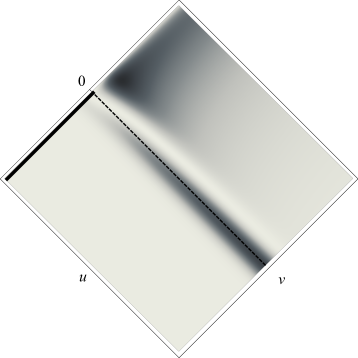
Figure 5: Plot of $|\Psi(u,v)|^{2}$ showing the scattering of a Gaussian wave-packet with $\ell=1$ and centre at $v=0$ from the singularity of the $\Delta=1/2$ metric. Light-shaded regions correspond to $|\Psi|^{2}\approxeq 0$.

4 Discussion

This final section will be a speculative discussion about the possible role of the linear Vaidya metric in the final stages of black hole evaporation. It will necessarily be much more qualitative than the preceeding sections, but we believe that the general semi-classical picture for the final stages of black hole evaporation should have features similar to that which we will present here.

As we do not have control over the late stages of the evolution of the Schwarzschild black-hole we will assume that there is a Planckian sized transition region between the lines $s$ and $s^{\prime}$ in figure (6), interpolating from a near Planck-mass Schwarzschild black hole to a linear mass Vaidya metric with $0<\mu<1/16$. To investigate the possible consistency of this proposal we will first look at the Kretschmann scalar as a measure of the magnitude of the curvature.

Figure 6: A blowup of the region $\mathcal{S}$ of figure (2).

For a Schwarzschild black hole of mass $M$

$$K_{\text{S}}=\frac{48G^{2}M^{2}}{r^{6}}$$ (4.1)

while for Vaidya

$$K_{\text{V}}=\frac{48\mu^{2}u^{2}}{r^{6}}.$$ (4.2)

We propose that the linear mass Vaidya metric should be inserted at a point in the evaporation where the stretched horizon at $r=G(2M+M_{\text{Pl}})$ meets the photon sphere of the Vaidya metric at $z=z_{\text{max}}$ and at this point the strength of the curvatures of Schwarzschild and Vaidya should be similar. Furthermore, continuity of the radius of the transverse sphere requires that the radial coordinates in Schwarzschild and Vaidya coincide in the matching region $\mathcal{T}$. Looking at the Kretschmann scalar we thus require that

$$\frac{M}{2M+M_{\text{Pl}}}=\mu z_{\text{max}}=\frac{1}{6}(1+\sqrt{1-12\mu}).$$ (4.3)

Introducing mass measured in Planck units $\bar{M}=M/M_{\text{Pl}}$ we find

$$\frac{6\bar{M}}{2\bar{M}+1}=1+\sqrt{1-12\mu},$$ (4.4)

and this implies that

$$\mu=\frac{\bar{M}(1-\bar{M})}{(2\bar{M}+1)^{2}}.$$ (4.5)

In addition we would also like the heights of the photon sphere barriers to be similar in the cross-over region and thus

$$\frac{1}{27\bar{M}^{2}}=h_{\text{max}}(\mu),$$ (4.6)

or solving for $\mu$,

$$\mu=-9\bar{M}^{2}-216\bar{M}^{4}+\sqrt{\bar{M}^{2}+108\bar{M}^{4}+3888\bar{M}^{6}+46656\bar{M}^{8}}.$$ (4.7)

Solving (4.5) and (4.7) simultaneously gives $\bar{M}=0.5086\approx 1/2$ at $\mu=0.0614<1/16$, indicating that the ideal matching point is close to $M=M_{\text{Pl}}/2$. If we consider only the matching of the Kretschmann scalar we find that we are restricted to a crossover from Schwarzschild to Vaidya that takes place in the interval $M_{\text{Pl}}/2<M<M_{\text{Pl}}$ corresponding to $0<\mu<1/16$. However, from (4.5), we see that increasing the mass at the transition region towards $M=M_{\text{Pl}}$ corresponds to $\mu\rightarrow 0$. In this limit we find that the height of the photon barrier of Schwarzschild decreases as $1/(27\bar{M}^{2})\rightarrow 1/27$ whereas that of the Vaidya metric increases as $1/(27\mu^{2})\rightarrow\infty$. Note also that, from the discussion of the previous section, the potential for scattering near the singularity and with $v<0$ is more repulsive when $\Delta\rightarrow 1$ ($\mu\rightarrow 0$) as can be seen from (3.8) and in figure (4). If indeed the matching occurs closer to $M_{\text{Pl}}$ it is necessary that after the Page time [19], when the mass of the black hole is on the order of several times $M_{\text{Pl}}$, the space-time becomes modified such that the potential rises more rapidly. The ideal choice of transition region requires some more information about the evolution after the Page time.

At this point we would like to add a couple of comments on the stability and self-consistency of our construction. In [5] it has been argued that the null singularity of these metrics may be unstable to backscattering due to large blueshifts as particles approach the singularity. Back-scattered particles outside the photon sphere will generically have $\ell\neq 0$ and thus will feel the repulsive nature of the singularity possibly reducing the effect of potential blue-shifts. Furthermore, outgoing particles that come from the near horizon region can escape to infinity only if they can pass the photon sphere from the inside, implying that those that get out must have either an energy that is significantly transplanckian, or zero angular momentum. In turn this appears to imply that in the final stages of evaporation outgoing Hawking radiation will predominantly have angular momentum close to zero leading to an a posteriori justification for the use of the Vaidya metric and for its stability.

Another interesting effect of the linear mass Vaidya modification of the final phase of evaporation is a slight cooling down of the black hole to $T\sim 1/\sqrt{M}$ compared to the well-known $T\sim 1/M$ of Schwarzschild. This is still divergent for vanishing mass, but it should be noted that in [9] the inclusion of backreaction causes a more significant cooling down with a finite temperature at the end-point of evaporation.

Obviously this is not a complete analysis of the cross-over region but we believe that the picture we are presenting is quite plausible. To make this more concrete it would be interesting to search for a deformation of the linear mass Vadiya metric for which the stress energy tensor is only spherically symmetric in the final Planckian region and becomes more like the stress-energy tensor of Hawking radiation further in the null past, thus providing also a semi-classical model for the adiabatically evaporating Schwarzschild to linear mass Vaidya transition. Along these lines there is a proposal in [21] for an evolution from a Robinson-Trautmann metric to a Vaidya metric in the final phase of evaporation.

Finally it is worthwhile highlighting the appearance of a scale-invariant metric in the final stages of evaporation. It would be very interesting to further investigate the possible role of scale invariance in black hole production and evaporation. Some interesting examples in black hole physics where scale invariance can be found are Choptuik scaling [23] and the universality of scale-invariant metrics in the Penrose limit of space-like and null space-time singularities [24].

Acknowledgements I would like to thank M. Blau and D. Veberič for useful comments and discussions. I would also like to thank A. Sušnik for help with the figures.

References

- [1] P.C. Vaidya, Current Science 12 (1943) 183.
- [2] H.Stephani, D. Kramer, M. MacCallum, C. Hoenselaers and E. Herlt, Exact solutions of Einstein’s Field Equations, Second Edition (Cambridge University Press, Cambridge, England, 2002).
- [3] P.C. Vaidya, Nonstatic Solutions of Einstein’s Field Equations for Spheres of Fluids Radiating Energy, Phys. Rev. 83 (1951) 10.
- [4] B. Waugh and Kayll Lake, Double-null coordinates for the Vaidya metric, Phys. Rev. D 34 (1986) 2978.
- [5] B. Waugh and Kayll Lake, Backscattered radiation in the Vaidya metric near zero mass, Phys. Lett. A 116 (1986) 154.
- [6] J. Bicak and K.V. Kuchar, Null dust in canonical gravity, Phys. Rev. D 56 (1997) 4878, arXiv:gr-qc/9704053.
- [7] W.A. Hiscock, L.G. Williams and D.M. Eardley, Creation Of Particles By Shell Focusing Singularities, Phys. Rev. D 26 (1982) 751.
- [8] Y. Kuroda, Vaidya Space-time As An Evaporating Black Hole, Prog. Theor. Phys. 71 (1984) 1422.
- [9] R. Balbinot, The back reaction and the small-mass regime, Phys. Rev. D 33 (1986) 1611–1615.
- [10] E. Abdalla, C.B.M.H. Chirenti and A. Saa, Quasinormal modes for the Vaidya metric, Phys.Rev. D 74 (2006) 084029, arXiv:gr-qc/0609036.
- [11] J. Bicak and P. Hajicek, Canonical theory of spherically symmetric space-times with cross streaming null dusts, Phys. Rev. D 68 (2003) 104016, arXiv:gr-qc/0308013.
- [12] S.G. Ghosh and N. Dadhich, On naked singularities in higher-dimensional Vaidya space-times, Phys. Rev. D 64 (2001) 047501, arXiv:gr-qc/0105085.
- [13] T. Harko, Gravitational collapse of a hagedorn fluid in Vaidya geometry, Phys. Rev. D 68 (2003) 064005, arXiv:gr-qc/0307064.
- [14] F. Girotto and A. Saa, Semi-analytical approach for the Vaidya metric in double-null coordinates, Phys. Rev. D 70 (2004) 084014, arXiv:gr-qc/0406067.
- [15] H. Kawai, Y. Matsuo and Y. Yokokura, A Self-consistent Model of the Black Hole Evaporation, Int. J. Mod. Phys. A 28 (2013) 1350050, arXiv:1302.4733 [hep-th].
- [16] F. Fayos and R. Torres, Local behaviour of evaporating stars and black holes around the total evaporation event, Class. Quant. Grav. 27 (2010) 125011.
- [17] A.N.St. J. Farley and P.D. D’Eath, Vaidya space-time in black-hole evaporation, Gen. Rel. Grav. 38 (2006) 425, arXiv:gr-qc/0510040.
- [18] D.A. Lowe and L. Thorlacius, Pure states and black hole complementarity, Phys. Rev. D 88 (2013) 044012, arXiv:1305.7459 [hep-th].
- [19] D.N. Page, Information in black hole radiation, Phys. Rev. Lett. 71 (1993) 3743, arXiv:hep-th/9306083; D.N. Page, How fast does a black hole radiate information?, Int. J. Mod. Phys. D 3 (1994) 93.
- [20] W. Unruh, Collapse of radiating fluid spheres and cosmic censorship, Phys. Rev. D 31 (1985) 2693.
- [21] J. Podolsky and O. Svitek, Radiative spacetimes approaching the Vaidya metric, Phys. Rev. D 71 (2005) 124001, arXiv:gr-qc/0506016.
- [22] C. Gundlach, R.H. Price, J. Pullin, Late time behavior of stellar collapse and explosions: 1. Linearized perturbations, Phys. Rev. D. 49 (1994) 883.
- [23] M. W. Choptuik, Universality and scaling in gravitational collapse of a massless scalar field, Phys. Rev. Lett. 70 (1993) 9.
- [24] M. Blau, M.Borunda, M. O’Loughlin and G. Papdopoulos, The Universality of Penrose limits near space-time singularities, JHEP 0407 (2004) 068, arXiv:hep-th/0403252; M. Blau, M.Borunda, M. O’Loughlin and G. Papdopoulos, Penrose limits and space-time singularities, Class. Quant. Grav. 21 (2004) L43, arXiv:hep-th/0312029.