Graphics Processing Units Accelerated Semiclassical Initial Value Representation Molecular Dynamics

Abstract

This paper presents a Graphics Processing Units (GPUs) implementation of the Semiclassical Initial Value Representation (SC-IVR) propagator for vibrational molecular spectroscopy calculations. The time-averaging formulation of the SC-IVR for power spectrum calculations is employed. Details about the GPU implementation of the semiclassical code are provided. Four molecules with an increasing number of atoms are considered and the GPU-calculated vibrational frequencies perfectly match the benchmark values. The computational time scaling of two GPUs (NVIDIA Tesla C2075 and Kepler K20) respectively versus two CPUs (Intel Core i5 and Intel Xeon E5-2687W) and the critical issues related to the GPU implementation are discussed. The resulting reduction in computational time and power consumption is significant and semiclassical GPU calculations are shown to be environment friendly.

I Introduction

The exponentially increasing demand for advanced graphics solutions for many software applications including entertainment, visual simulation, computer-aided design and scientific visualization has boosted high-performance graphics systems architectural innovation.NVIDIA Nowadays, Graphics Processing Units (GPUs) are ubiquitous, affordable and designed to exploit the tremendous amount of data parallelism of graphics algorithms.

In recent years, GPUs have evolved into fully programmable devices and they are now ideal resources for accelerating several scientific applications. GPUs are designed with a philosophy which is very different from CPUs. On one hand, CPUs are more flexible than GPUs and able to provide a fast response to a single task instruction. On the other hand, GPUs are best performing for highly parallelized processes. CPUs provide caches and this hardware tool has been developed in a way to better assist programmers. In particular, caches are transparent to programmers and the recent bigger ones can capture most used data. GPUs, instead, achieve high performances by means of hundreds of cores which are fed by multiple independent parallel memory systems. A single GPU is composed of groups of single-instruction multiple-data (SIMD) processing units and each unit is made of multiple smaller processing parts called threads. These are set to execute the same instructions concurrently. The advantages of this type of architecture consist in a reduced power consumption and an increased number of floating point arithmetic units per unit area. In other words, a reduced amount of space, power and cooling is necessary to operate. However, parallelization efficiency depends critically on threads synchronization. In fact, accidental or forced inter-thread synchronization can turn out to be very costly, because it involves a kernel termination. Generation of a new kernel implies overhead from the host. Another GPU drawback is represented by its better efficiency for single precision arithmetics. Unfortunately, single precision is not enough for most scientific calculations. In general, then, there may not be a single stable GPU programming model and CPU codes need usually to be extensively changed in order to fit the GPU hardware.

GPUs are becoming more and more popular among the scientific community mainly thanks to the release of NVIDIA’s Compute Unified Device Architecture (CUDA) toolkit.CUDA This is a programming model based on a user-friendly decomposition of the code into grids and threads which significantly simplifies the code development. It allows to exploit all of the key hardware capabilities, such as scatter/gather and thread synchronizations.

Applications of GPU programming in theoretical chemistry include implementations for classical molecular dynamics (MD),Schulten_GPUMD_07 ; Schulten_2 ; Schulten_conference ; Elber2 quantum chemistry Martinez_2008 ; Yasuda ; Alan_JPCA_08 ; Genovese ; Alan_QuantumChemistryGPU_10 ; Tomono ; Genovese2 ; Alan_Rubio_12 ; Dronskowski ; Hammond ; QE_GPU ; Stotzka ; Maia ; Hacene ; Esler ; Hakala ; Jia ; Hutter , protein folding Pande_GPUfolding_13 , quantum dynamicsZerbetto_QMGPU_12 ; Han_scattering_13 ; Lagana1 ; Lagana2 ; Lagana3 ; Murgante and quantum mechanics / molecular mechanics (QM/MM) Maezono_QMMMGPU_11 simulations. For instance, classical MD can be sped up by using GPUs for the calculation of long-range electrostatics and non-bonded forces.Schulten_GPUMD_07 ; Schulten_2 The direct Coulomb summation algorithm accesses the shared memory area only at the very beginning and the very end of the processing for each thread block, so MD takes full advantage of the GPUs architecture by eliminating any use of thread synchronizations. For instance, the popular Not (just) Another Molecular Dynamics (NAMD) program Schulten_2 ; Schulten_conference is accelerated several times by directing the electrostatics and implicit solvent model calculations to GPUs while the remaining tasks are handled by CPUs. Significant progress by Friedrichs et al. has determined a MD speed up of about 500 times over an 8-core CPU by using the OpenMM library.Friedrichs More difficult has been the adoption of GPUs for quantum chemistry. The first full electronic-structure implementation on GPUs was Ufimtsev and Martinez’s TeraChem.Martinez_2008 Currently, there are several electronic structure codes that have to some extent implemented GPU accelerations.Yasuda ; Alan_QuantumChemistryGPU_10 ; QE_GPU For example, Aspuru’s group successfully accelerated real-space DFT calculations making this approach interesting and competitive.Alan_JCTC_13_realspaceDFT A simple GPU implementation of the Cublas SGEMM subroutine in quantum chemistry has been shown to be about 17 times faster than the parent DGEMM subroutine on CPU.Alan_QuantumChemistryGPU_10 Recently, CPU/GPU-implemented time-independent quantum scattering calculations featured a 7-time acceleration by employing 3 GPU and 3 CPU cores.

In a time-dependent quantum propagation, instead, almost all of the computational resources are spent for the time propagation of the wavepacket. Only the initial wavepacket is calculated on the CPU. Data are copied from the CPU memory to the GPU one for wavepacket propagation. Furthermore, it has been shown that quantum time-dependent approaches can be boosted up to two orders of magnitude by taking advantage of the matrix-matrix multiplication for the time-evolution that maps well to GPU architectures.Zerbetto_QMGPU_12 ; Han_scattering_13 Lagana’s group demonstrated that quantum reactive scattering for reactive probabilities calculations can be accelerated as much as 20 times.Lagana1 ; Lagana2 ; Lagana3 ; Lagana_Pacifici_13

The main goal of this paper is to speed up our semiclassical dynamics CPU code by exploiting the GPU hardware. We show how and when it is convenient to employ GPU devices to perform semiclassical simulations. The GPU approach is also demonstrated to require a largely reduced amount of power supply. Unfortunately, GPU accelerated programming experiences gained for quantum propagation matrix-matrix multiplications or for the classical Coulombic MD force field are not helpful in the case of semiclassical simulations, due to the need to calculate concurrently quantum delocalization and classical localization. Given the mixed classical and quantum nature of the semiclassical propagator, a general purpose (GP) GPU approach is taken. With this approach host codes run on CPUs and kernel codes on GPUs. GPGPU programming is principally aimed at minimizing data transfer between the host and the kernel, since this communication is made via bus with relatively low speed.

The paper is organized as follows. Next Section recalls the semiclassical initial value representation quantum propagator and the following one describes the GPGPU programming approach adopted here. The Section compares the performances of CPU and GPGPU codes and discusses them. The last Section reports our conclusions.

II Semiclassical initial value representation of the quantum propagator

The semiclassical propagator can be derived from the Feynman Path Integral formulation of the quantum evolution operator Feynman_Hibbs from point $\mathbf{q}$ to $\mathbf{q}^{\prime}$

$$\mbox{$\left\langle\mathbf{q}^{\prime}\left|e^{-i\hat{H}t/\hbar}\right|\mathbf{q}\right\rangle$}=\left(\frac{m}{2\pi i\hbar t}\right)^{1/2}\int\mathcal{D}\left[\mathbf{q}\left(t\right)\right]e^{iS_{t}\left(\mathbf{q},\mathbf{q}^{\prime}\right)/\hbar}$$ (1)

where $S_{t}\left(\mathbf{q},\mathbf{q}^{\prime}\right)$ is the path action for time $t$ and $\mathcal{D}\left[\mathbf{q}\left(t\right)\right]$ indicates the differential over all paths. Stationary phase approximation of Eq. (1) (see, for instance, Ref. 37; 38) yields the semiclassical van Vleck-Gutzwiller propagatorvanVleck_PNAS ; Gutzwiller_SCpropagator

$$\left\langle\mathbf{q}^{\prime}\left|e^{-i\hat{H}t/\hbar}\right|\mathbf{q}\right\rangle\approx\sum_{\mbox{roots}}\left[\frac{1}{\left(2\pi i\hbar\right)^{F}}\left|-\frac{\partial^{2}S}{\partial\mathbf{q}^{\prime}\partial\mathbf{q}}\right|\right]^{1/2}e^{iS_{t}\left(\mathbf{q},\mathbf{q}^{\prime}\right)/\hbar-i\nu\pi/2}$$ (2)

where the sum is over all classical trajectories going from $\mathbf{q}$ to $\mathbf{q}^{\prime}$ in an amount of time $t$, $F$ is the number of degrees of freedom, and $\nu$ is the Maslov or Morse index, i.e. the number of points along the trajectory where the determinant in Eq. (2) diverges.Morse ; Maslow To apply Eq. (2) as written, one needs to solve a nonlinear boundary value problem. The classical trajectory evolved from the initial phase space point $\left(\mathbf{p}\left(0\right),\mathbf{q}\left(0\right)\right)$ is such that $\mathbf{q}_{t}\left(\mathbf{p}\left(0\right),\mathbf{q}\left(0\right)\right)=\mathbf{q}^{\prime}$. In general, there will be multiple roots to this equation and the summation of Eq. (2) is over all such roots. Finding these roots is a formidable task that has hindered use and diffusion of semiclassical dynamics. The issue was overcome by Miller’s Semiclassical Initial Value Representation (SC-IVR), whereby the boundary condition summation is replaced by an initial phase space integration amenable to Monte Carlo implementation.Miller_IVR ; Grossmann_avd ; Kay_IVR ; Pollak ; ContePollak10 ; ContePollak12 ; Jiri By representing the van Vleck-Gutzwiller propagator by direct product of one-dimensional $\gamma_{i}$-width coherent states Kay_IVR ; Heller_frozengaussian ; HermanKlukcoherstates ; SunMiller_HCldimer ; Miller_JPC_featurearticle ; Miller_PNAS defined by

$$\left\langle\mathbf{q}|\mathbf{p}\left(t\right),\mathbf{q}\left(t\right)\right\rangle =\prod_{i}\left(\mathbf{\gamma}_{i}/\pi\right)^{F/4}$$

$$\times \mbox{exp}\left[-\frac{\gamma_{i}}{2}\left(q_{i}-q_{i}\left(t\right)\right)^{2}+\frac{i}{\hbar}p_{i}\left(t\right)\left(q_{i}-q_{i}\left(t\right)\right)\right]$$ (3)

and using Miller’s IVR trick, the semiclassical propagator becomes

$$e^{-i\hat{H}t/\hbar}= \frac{1}{\left(2\pi\hbar\right)^{F}}\int d\mathbf{p}\left(0\right)\int d\mathbf{q}\left(0\right)\>C_{t}\left(\mathbf{p}\left(0\right),\mathbf{q}\left(0\right)\right)$$ (4)

$$e^{iS_{t}\left(\mathbf{p}\left(0\right),\mathbf{q}\left(0\right)\right)/\hbar}\left|\mathbf{p}\left(t\right),\mathbf{q}\left(t\right)\left\rangle\right\langle\mathbf{p}\left(0\right),\mathbf{q}\left(0\right)\right|.$$

$\left(\mathbf{p}\left(t\right),\mathbf{q}\left(t\right)\right)$ represent the set of classically-evolved phase space coordinates and $C_{t}$ is a pre-exponential factor. In the Herman-Kluk frozen Gaussian version of SC-IVR, the pre-exponential factor is written asKay_IVR ; Heller_frozengaussian ; HermanKlukcoherstates

$$C_{t}\left(\mathbf{p}\left(0\right),\mathbf{q}\left(0\right)\right) =$$ (5)

$$\sqrt{\frac{1}{2}\left|\frac{\partial\mathbf{q}\left(t\right)}{\partial\mathbf{q}\left(0\right)}+\frac{\partial\mathbf{p}\left(t\right)}{\partial\mathbf{p}\left(0\right)}-i\hbar\Gamma\frac{\partial\mathbf{q}\left(t\right)}{\partial\mathbf{p}\left(0\right)}+\frac{i}{\Gamma\hbar}\frac{\partial\mathbf{p}\left(t\right)}{\partial\mathbf{q}\left(0\right)}\right|}$$

where $\Gamma=\mbox{diag}\left(\gamma_{1},...,\gamma_{F}\right)$ is the coherent state matrix which defines the Gaussian width of the coherent state. The calculation of C_t is conveniently performed from blocks of size $F\times F$ by introducing a $2F\times 2F$ symplectic (monodromy or stability) matrix $\mathbf{M}\left(t\right)\equiv\partial\left(\left(\mathbf{p}_{t},\mathbf{q}_{t}\right)/\partial\left(\mathbf{p}_{0},\mathbf{q}_{0}\right)\right)$. The accuracy of time-evolved classical trajectories is monitored by calculating the deviation of the determinant of the positive-definite matrix $\mathbf{M}^{T}\mathbf{M}$ from unity.Miller340_GeneralizedFilinov_01 In this work, a trajectory is discarded when its deviation is greater than $10^{-6}$. For semiclassical dynamics of bound systems, a reasonable choice for the $\gamma_{i}$ width parameters is provided by the harmonic oscillator approximation to the wave function at the global minimum.

In this paper, we employ the SC-IVR propagator to calculate the spectral density

$$I\left(E\right)\equiv\left\langle\chi\left|\delta\left(\hat{H}-E\right)\right|\chi\right\rangle=\sum_{n}\left|\left\langle\chi|\psi_{n}\right\rangle\right|^{2}\delta\left(E-E_{n}\right),$$ (6)

where $\left|\chi\right\rangle$ is some reference state, $\left\{\left|\psi_{n}\right\rangle\right\}$ are the exact eigenfunctions and $\left\{E_{n}\right\}$ the corresponding eigenvalues of the Hamiltonian $\hat{H}$. A more practical dynamical representation of Eq. (6) is given by the following time-dependent representationHeller_review_autocorrel ,

$$I\left(E\right)=\frac{1}{2\pi\hbar}\int_{-\infty}^{+\infty}\left\langle\chi\left|e^{-i\hat{H}t/\hbar}\right|\chi\right\rangle e^{iEt/\hbar}dt=\frac{\mbox{Re}}{\pi\hbar}\int_{0}^{+\infty}\left\langle\chi\left|e^{-i\hat{H}t/\hbar}\right|\chi\right\rangle e^{iEt/\hbar}dt$$ (7)

which is obtained by replacing the Dirac delta function in Eq. (6) by its Fourier representation. According to Eq. (7) and Eq. (4), the SC-IVR spectral density representation becomesMiller312_FaradayDisc_98

$$I\left(E\right) = \frac{1}{2\pi\hbar}\int_{-\infty}^{+\infty}e^{iEt/\hbar}\frac{1}{\left(2\pi\hbar\right)^{F}}\int d\mathbf{p}\left(0\right)\int d\mathbf{q}\left(0\right)\>C_{t}\left(\mathbf{p}\left(0\right),\mathbf{q}\left(0\right)\right)$$ (8)

$$\times e^{iS_{t}\left(\mathbf{p}\left(0\right),\mathbf{q}\left(0\right)\right)/\hbar}\left\langle\chi|\mathbf{p}\left(t\right),\mathbf{q}\left(t\right)\right\rangle\left\langle\mathbf{p}\left(0\right),\mathbf{q}\left(0\right)|\chi\right\rangle dt$$

where the reference state $\left|\chi\right\rangle=\left|\mathbf{p}_{eq},\mathbf{q}_{eq}\right\rangle$ is represented in phase space coordinates. The Monte Carlo phase space integration is made easier to treat by introducing a time averaging filter at the cost of a longer simulation time. This implementation was introduced by Kaledin and MillerAlex resulting in the following time-averaging (TA) SC-IVR formulation for the spectral density

$$I\left(E\right) = \frac{1}{\left(2\pi\hbar\right)^{F}}\int d\mathbf{p}\left(0\right)\int d\mathbf{q}\left(0\right)\frac{\mbox{Re}}{\pi\hbar T}\int_{0}^{T}dt_{1}\int_{t_{1}}^{T}dt_{2}\>C_{t_{2}}\left(\mathbf{p}\left(t_{1}\right),\mathbf{q}\left(t_{1}\right)\right)$$ (9)

$$\times \left\langle\chi\left|\right.\mathbf{p}\left(t_{2}\right),\mathbf{q}\left(t_{2}\right)\right\rangle e^{i\left(S_{t_{2}}\left(\mathbf{p}\left(0\right),\mathbf{q}\left(0\right)\right)+Et_{2}\right)/\hbar}\left[\left\langle\chi\left|\right.\mathbf{p}\left(t_{1}\right),\mathbf{q}\left(t_{1}\right)\right\rangle e^{i\left(S_{t_{1}}\left(\mathbf{p}\left(0\right),\mathbf{q}\left(0\right)\right)+Et_{1}\right)/\hbar}\right]^{*}.$$

Eq. (9) presents two time variables. The integration over $t_{2}$ is taking care of the Fourier transform of Eq. (7) (limited to the simulation time T), while the one over $t_{1}$ does the filtering job. The positions $\left(\mathbf{p}\left(t_{1}\right),\mathbf{q}\left(t_{1}\right)\right)$ and $\left(\mathbf{p}\left(t_{2}\right),\mathbf{q}\left(t_{2}\right)\right)$ are referred to the same trajectories but at different times. By adopting a reasonable approximation for the pre-exponential factor, $C_{t_{2}}\left(\mathbf{p}\left(t_{1}\right),\mathbf{q}\left(t_{1}\right)\right)=\mbox{Exp}\left[i\left(\phi\left(t_{2}\right)-\phi\left(t_{1}\right)\right)/\hbar\right],$Alex where $\phi\left(t\right)=\mbox{phase}\left[C_{t}\left(\mathbf{p}\left(0\right),\mathbf{q}\left(0\right)\right)\right]$, the double-time integration of Eq. (9) is reduced to a single one and the spectral density becomes

$$I\left(E\right) = \frac{1}{\left(2\pi\hbar\right)^{F}}\frac{1}{2\pi\hbar T}\int d\mathbf{p}\left(0\right)\int d\mathbf{q}\left(0\right)$$

$$\times \left|\int_{0}^{T}dt\left\langle\chi|\mathbf{p}\left(t\right),\mathbf{q}\left(t\right)\right\rangle\right.$$

$$\times \left.e^{i\left(S_{t}\left(\mathbf{p}\left(0\right),\mathbf{q}\left(0\right)\right)+Et+\phi_{t}\left(\mathbf{p}\left(0\right),\mathbf{q}\left(0\right)\right)\right)/\hbar}\right|^{2}.$$

Eq. (II) offers the advantage that the integrand is now positive-definite and the integration is less computationally demanding. Several applicationsAlex ; Ceotto_1traj ; Ceotto_MCSCIVR ; Ceotto_david ; Ceotto_eigenfunctions ; Ceotto_cursofdimensionality_11 ; Ceotto_acceleratedSCIVR ; Ceotto_NH3 have demonstrated that this approximation is quite accurate.

III GPU Implementation of the SC-IVR Spectral Density

III.1 Monte-Carlo SC-IVR algorithm

To point out the degree of parallelism available in the SC-IVR procedure, we describe the main steps that lead to the computation of the semiclassical power spectrum.
The spectrum is conveniently represented as a $k$-dimensional vector $\left(E_{1}=E_{min},E_{2},...,E_{k}=E_{max}\right)$ of equally spaced points in the range $[E_{min},E_{max}]$. To evaluate each element of the discretized spectrum we need to calculate $I(E_{i}),\,i=1,2,\ldots,k$ from Eq. (II). To this end we use a Monte Carlo (MC) method. The phase-space integral of Eq. (II) is approximated by means of the following MC sum of $n_{traj}$ classical trajectories

$$I(E_{i})=\frac{1}{\left(2\pi\right)^{F+1}}\frac{1}{n_{good}T}\sum_{j=1}^{n_{traj}}w_{j}\left|\sum_{c=0}^{n_{steps}}\left\langle\chi\left|\mathbf{p}_{j}(c\Delta t),\mathbf{q}_{j}(c\Delta t)\right.\right\rangle e^{i\left(S_{c\Delta t}\left(\mathbf{p}_{j}\left(0\right),\mathbf{q}_{j}\left(0\right)\right)+E_{i}c\Delta t+\phi_{c\Delta t}\left(\mathbf{p}_{j}\left(0\right),\mathbf{q}_{j}\left(0\right)\right)\right)}\right|^{2}$$ (11)

where atomic units have been employed, and $n_{good}$ is the actual number of trajectories ($n_{good}\leq n_{traj}$) over which the sum is averaged, as discussed at the end of next paragraph. The MC phase space sampling is performed according to the Husimi distribution which determines the weight $w_{j}$ of each trajectory.Alex The classical trajectories $\left(\mathbf{p}_{j}(t),\mathbf{q}_{j}(t)\right)$ and the actions are then evolved, through $n_{steps}$ discrete time steps of length $\Delta t$ from time $0$ to time $T$ by means of a fourth order symplectic algorithm.Ceotto_HessianAccuracy
The structure of the sequential (CPU) code is shown in Fig. 1.

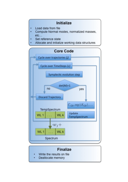
Figure 1: The structure of the sequential code.

First, all the relevant information about the molecule under investigation are read from the configuration files. These are the masses and the equilibrium positions of the atoms. Then, normal mode coordinates are generated together with the conversion matrix from normal modes to Cartesian coordinates. This matrix is necessary, since the simulations are performed in normal mode coordinates, while the potential subroutines are written in Cartesian or Internal coordinates. Once all the simulation and molecule-configuration parameters have been loaded into the program, the sequential generation of MC trajectories starts. In order to check the stability of the symplectic evolution of each trajectory, the determinant of the monodromy matrix $\left|M(t)\right|$ is evaluated. As soon as it deviates from unity by an amount greater than $10^{-6}$, the evolution of the trajectory is interrupted and its contribution to the MC integration discarded. The intermediate results produced by the trajectory are stored in a buffer (TempSpectrum). The buffered results contribute to the computation of the spectrum(which is done in the Spectrum array) only if the trajectory has completed its evolution over the whole $[0,T]$ time interval. We use a counter $n_{good}$ to count the number of "good" trajectories. When all the trajectories have been generated, the spectrum is normalized over $n_{good}$ and copied into a file.

III.2 GP-GPU Implementation

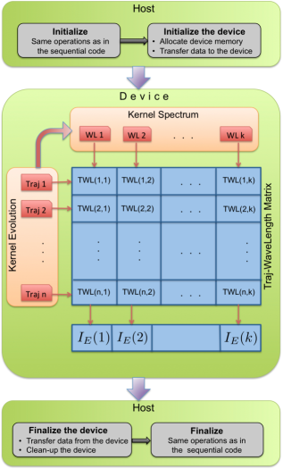
(a) CUDA code structure. The $j$-th row $(TW(j,1),TW(j,2),\ldots,TW(j,k))$ of the Traj-WaveLength matrix contains the private copy of the TempSpectrum array of the $j$-th trajectory. After the threads of KernelEvolution have filled the matrix, KernelSpectrum is launched. Each thread of KernelSpectrum performs the sum of the elements over each column of Traj-WaveLength.

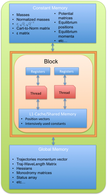
(b) Use of the memory hierarchy while executing the Evolution Kernel.

Figure 2:

Since each trajectory evolves independently, the design of a parallel version of the MC algorithm described in Eq. (11) is rather straightforward. As the most direct implementation, a $n_{traj}$ simulation can be performed by means of $n_{traj}$ independent computational units, each one working on a private memory space. Once all the trajectories have been run, the results can be summed up to obtain the final spectrum. Here, we describe the implementation of the MC SC-IVR algorithm for $\mbox{NVIDIA}^{\text{\textregistered}}$ GP-GPU with compute capability $\geq 2.0$ . Double precision floating point operations are supported. Therefore, we can adopt the terminology of NVIDIA CUDA. The design guidelines that we are going to introduce can also be implemented on other GP-GPUs and more generally on any Single Instruction Multiple Data (SIMD) architectures, e.g. through OpenCLKhronos
The present parallel implementation of the SC-IVR algorithm uses two kernels, which are the Evolution Kernel (KernelEvolution in the code and in Fig. 2a) and the Spectrum Kernel (KernelSpectrum in the code and in Fig. 2a). In the Evolution Kernel the cycle over the trajectories (see Fig. 1) is distributed over a number of $n_{traj}$ threads. The $j$-th thread evolves a given initial condition $\left(\mathbf{p}_{j}(0),\mathbf{q}_{j}(0)\right)$ from time $0$ to time $T$ and works on its private copy of the working variables used in the sequential code. Details about the memory usage will be presented below. In order to avoid instruction branching, which is highly detrimental in the SIMD setup, all the trajectories are evolved up to time $T$. The trajectory status is monitored by means of a flag variable which is initialized to good and switched to bad as soon as the determinant of the monodromy matrix associated to the trajectory deviates from the allowed tolerance. Information about the spectrum contributed by each trajectory during its evolution are stored in its private copy of the buffer array. We organize these private copies into the $n_{traj}\times k$ buffer matrix (Traj-WaveLength in Fig. 2a).
When the Evolution kernel terminates, the Spectrum kernel is launched with $k$ threads. At the end of the time evolution, the $j$-th thread computes the weighted sum of the elements of the $j$-th column of the buffer matrix. The results of bad trajectories are not considered by setting their weight to zero. The structure of the CUDA code just described is shown in Fig. 2a. The main advantage of using two separate kernels is that we are able to take into account the different dimensions of the problem, that is the number $n_{traj}$ of MC trajectories and the number $k$ of sampled energies. Another advantage is that the threads work always on separate memory locations, making therefore unnecessary the use of atomic operations or any other kind of thread synchronization mechanism that otherwise would slash the performance of the parallel code.

A central task in the development of CUDA coding concerns the optimization of the use of different types of GPU memories. As a matter of fact, memory bandwidth can be the real bottleneck in a GPGPU computation. As mentioned above, in order to reproduce the independence on the MC trajectory in the code, each thread works on a private copy of variables. On one hand, this could be easily accomplished by reserving to each thread a portion of consecutive Global Memory words large enough to contain all its working variables. On the other hand, this naive approach would lead to highly misaligned memory accesses and to a large amount of unnecessary and costly memory traffic. In order to allow for coalesced read/write operations in the global memory, we store the $n_{traj}$ copies of the same variable in contiguous positions. For instance, the momenta of the different MC trajectories are stored as $\left(p_{1}^{1},p_{2}^{1},...,p_{n_{traj}}^{1},...,p_{1}^{F},p_{2}^{F},...,p_{n_{traj}}^{F}\right)$, where $F$ is the number of degrees of freedom (the normal modes) of the molecule. In this way neighbor threads will issue read/write memory requests to neighbor memory locations that can be "simultaneously" served.

We recall that atom masses, equilibrium positions, the conversion matrix and other potential-structure matrices are constant and trajectory-independent. Thus, we store these parameters in the Constant Memory. In this way, when all the threads in an half-warp issue a “read” of the same constant memory address, i.e. for the same parameter, a single “read” request is generated and the result is broadcasted to all the requiring threads. Moreover, since constant memory is cached, all the subsequent requests of the same parameter by other threads will not generate memory traffic.

Finally, we discuss the matter of the L1-Cache/shared memory usage. This 64kB memory is located close (on chip) to the processing units (CUDA cores) and provides the lowest latency times. By default, 16kB of this memory are used as L1-Cache memory, which is automatically managed by the device, whereas the remaining 48kB can be used either to share information between the threads in a block or as a "programmable cache". Since there is no flow of information between threads, we use the shared memory as "programmable" cache. Due to the limited size of this memory, we employ it to store only the position vectors of the trajectories in a block and some intensively used parameters. Fig. (2b) shows where the main data structures employed by the code are allocated.

We conclude this Section with a remark about the block-versus-thread structure. The threads that are used to generate the MC trajectories or to compute the components of the spectrum are evenly distributed among the blocks. The number of blocks, therefore, determines the threads/block ratio. Taking into account the dimension of the scheduling unit (warp), we constrain the number of threads-per-block to be an integer multiple of 32. Subsequently, we choose the configuration that provides the best performance, i.e. the shortest computing time. This procedure allows us to slash most of memory latency times and guarantees a sufficient number of Registers for each thread as well.

IV Results and discussion

Initially, debugging calculations are performed with GPU $\mbox{NVIDIA}^{\text{\textregistered}}\mbox{Tesla}^{\mbox{TM}}\mbox{C2075}$ and CPU Intel core i5-3550 (6M Cache, 3.3GHz) processors. Then, performance calculations are done employing the GPU $\mbox{NVIDIA}^{\text{\textregistered}}\mbox{Kepler}^{\mbox{\text{\textregistered}}}\mbox{K20}$ and CPU Intel Xeon E5-2687W (20M Cache, 3.10 GHz) at the Eurora cluster of the Italian supercomputer center CINECA.
In order to avoid any accidental over-estimation of the GPU code performance, we stress that the CPU code uses a single thread and does not make any use of SIMD instruction sets, such as Intel SSE. This means that the CPU code is not designed to fully exploit the computational power of multi-core or SSE-enabled processors. Considered the parallel nature of the described MC algorithm, a multi-thread version of the code will require in the best case $1/k$ of the single-thread CPU time, where $k$ is the number of available cores.
As for GPUs, we use the same code on both Tesla C2075 and K20, with the exception of the block vs thread configuration that is set to maximize the performance on each device. The new functionalities introduced by the Kepler architecture (such as dynamic parallelism and the 48K Read-Only Data Cache) are not exploited.

In order to test the performance of the CUDA SC-IVR code described in the previous section, we look at four molecules with an increasing number of degrees of freedom. It is important to study the time scaling not only for increasing number of trajectories, but also for increasing complexity of the molecular system. The chosen molecules are $\mbox{H}_{2}$, $\mbox{H}_{2}\mbox{O}$, $\mbox{H}_{2}\mbox{CO}$, and $\mbox{C}\mbox{H}_{2}\mbox{D}_{2}$ and the number of their vibrational degrees of freedom is respectively 1, 3, 6, and 9. So, one should keep in mind that the vibrational mode number grows at the fast pace of three times the number of atoms. Another aspect to take into account for a proper time scaling evaluation is represented by the potential energy subroutine adopted. For the $\mbox{H}_{2}$ molecule, a simple Morse oscillator is employed, while for the other molecules we use analytical potential energy surfaces fitted to ab initio quantum electronic energies.PES_H2O ; PES_H2CO ; PES_CH2D2

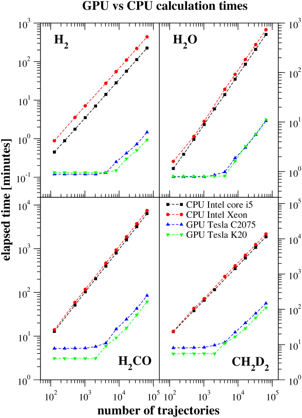
Figure 3: Elapsed computational time for CPU-SCIVR and GPU-SCIVR calculations. For a small number of trajectories (<2048), GPU times are roughly constant: the GPUs computational capabilities are not fully exploited. For a large number of trajectories (>>4096) GPU times scale linearly with respect to the number of trajectories. CPU times grow linearly with the number of trajectory on the whole range $[128,65536]$.

We are aware that about one thousand trajectories per vibrational degree of freedom Alex are necessary in order to reach convergence in the Monte Carlo integration of Eq. (II). However, we report calculations performed up to 65536 trajectories. This allows for a study of computing capability saturation of the two GPUs under consideration (see below) as well as a better description of the different computational simulation time trends of CPUs and GPUs. Fig. 3 shows the computational time at different numbers of classical trajectories and for different molecules. Semiclassical CPU calculations show a linear scaling up to the maximum number of 65536 trajectories tested. Instead, the computational time of the SC-IVR GPU CUDA code described above is roughly constant up to $n_{traj}=2048$ for K20 and $n_{traj}=4096$ for C2075, independently of the molecule under investigation. While the serial operation modality enforced by CPU architecture is clearly at the origin of the linear scaling, the GPU behaviour is a more sophisticated one. As a matter of fact, the execution time for a number of trajectories smaller than the indicated thresholds (2048/4096) is very close to the time required by the GPU to complete the evolution of a single trajectory. By accurately profiling the execution of the code, we find that this behaviour is largely due to the high memory traffic generated by the code, since a single trajectory requires the manipulation of a large number of data. Thanks to an accurate memory mapping of the information needed by the code (see below), we are able to minimize the on-chip/off-chip data transfer. We find that the latency-time (i.e. the amount of time required for data to become available to a thread) is playing a central role. However, when the number of threads is larger than the number of Streaming Multiprocessors (the computational units in CUDA), part of the latencies is hidden by the thread scheduler. Instead, when a thread is inactive while waiting for data to arrive, another one, which is ready for execution, is run. The execution time ceases to remain constant as soon as the number of threads becomes larger than the time needed to hide the latencies. This occurs when the computational power of the GPU is saturated. Interestingly enough, the "more powerful" K20 gets saturated sooner (2048 threads) than the "old" C2075. We will address this issue later in this section.

For every molecular system, once the number of trajectories is large enough for the Monte Carlo integral to converge, the resulting power spectrum is compared to the one reported by Kaledin and Miller.Alex We find our eigenvalues to be in agreement within 0.1%. This negligible discrepancy is due to the slightly different number of trajectories used in the GPU calculations.

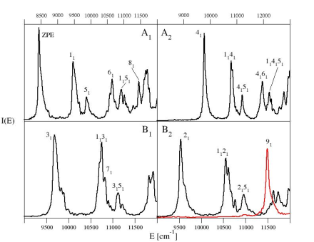
Figure 4: The deuterated methane $\mbox{CH}_{2}\mbox{D}_{2}$ power spectrum using the K20 GPU. The MC integration was converged with 8192 trajectories and the spectrum has been projected onto the four irreducible representations for a peak attribution. Red and black lines are different coherent state combinations for the same irreducible representation.

As an example, we report in Fig. 4 the power spectrum of di-deuterated methane. We stress once more that our main goal is to test accuracy and efficiency of the GPU implemented SC-IVR code and not just the determination of the spectrum, a problem which has already been solved. In Fig. 4, the power spectrum of the deuterated methane $\mbox{CH}_{2}\mbox{D}_{2}$ is projected onto the irreducible representations of the relevant molecular point group. This procedure helps the reader, assists the authors to assign peaks more easily and permits a stricter comparison with previous calculations on the same systems.Alex ; Ceotto_cursofdimensionality_11

After verifying that indeed the GPU implemented code preserves the same accuracy of the CPU one, we turn to the computational performance difference between the two NVIDIA graphics units, i.e. C2075 and K20. Clearly, for each molecule tested, one would expect a better performance of the more recent K20 with respect to C2075, as reported in Fig. 5.

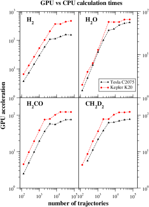
Figure 5: NVIDIA graphics units C2075 and K20 performances respectively versus the Intel Core i5 and the Intel Xeon E5-2687W for the calculation of the power spectra.

The acceleration amount shown in Fig. 5 increases with the number of trajectories. The upper left panel of the Figure reports the speed-up for the Morse oscillator power spectrum calculation. The acceleration is comparable in magnitude for the water molecule presented on the upper right panel and the two graphics units performances are quite similar. Instead, for the complex systems reported on the lower panels, the acceleration of the K20 graphic card is larger, as pointed out by the log-scale.

The trends of computational time (see Fig. 3) and acceleration beyond $n_{traj}=2048$ for K20 and $n_{traj}=4096$ for C2075 deserve some further discussion. As mentioned above, for a given number $n_{traj}$ of MC trajectories, the number of threads per block configuration is always chosen to maximize the performance. This number is usually kept high enough to make it possible for the warp scheduler to hide memory access latency. We find out that for $256\leq n_{traj}\leq 8192$ the best results are obtained with 128 threads in each block, independently of the device we run the code on. The real occupancy, i.e. the number of warps (execution units of 32 threads) running concurrently on a multiprocessor, however, is determined by the register needed by each thread. This is a key issue when codes are using a high number of variables, like in the present case. The dimension of the SMX register file is twice the size of the register memory for C2075 (256kB vs. 128kB), so the occupancy of K20 can be higher than that of C2075. On one side, this contributes to speed-up the calculations as shown by the K20 device performances. On the other side, the size of the L1 cache memory we use (48kB) is the same on both devices. This means that the same amount of L1 cache is shared among more really concurrent threads on K20 than on C2075. This results in a higher on-chip/off-chip memory traffic, and it is likely a reason for the earlier reduction of the GPU acceleration growth rate of Kepler K20 with respect to Tesla C2075.

Table 1: Performance of each computing device.^a)

Molecule	i5-3550	C2075	ratio CPU/GPU	E5-2687W	K20	ratio CPU/GPU
$\mbox{H}_{2}$	28.20b)	0.25	113	55.03	0.15	367
$\mbox{H}_{2}\mbox{O}$	73.63	1.87	39	91.60	1.62	57
$\mbox{H}_{2}\mbox{CO}$	798.07	14.42	55	936.73	9.18	102
$\mbox{CH}_{2}\mbox{D}_{2}$	1428.35	22.35	64	1715.73	16.63	103

$a)$ The number of trajectories is 65536. $b)$ The computational time is measured in minutes.

Table 1 reports the computational time for the fully converged TA-SC-IVR spectra calculations for the devices employed. This Table shows that the K20 computational time is always smaller than that of the older C2075 and of any other CPU device.

If we consider the computational time for the better performing K20 GPU and look at the time scaling for all the molecules under examination, we obtain the plot reported by the black filled circles in Fig. 6.

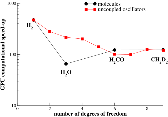
Figure 6: Power spectrum GPU computational speed-up for $\mbox{H}_{2}$, $\mbox{H}_{2}\mbox{O}$, $\mbox{H}_{2}\mbox{CO}$, and $\mbox{C}\mbox{H}_{2}\mbox{D}_{2}$ (filled black circles) compared to uncoupled Morse oscillators (filled red squares) with the same number of degrees of freedom and for a 65536 trajectory Monte Carlo integration.

Opposite to what one would expect, the ratio of the CPU computational time over the GPU one is not monotonically decreasing with the number of vibrational degrees of freedom for the molecule calculations. To find the source of such an irregular behavior, we treat a set of uncoupled Morse oscillators. We calculate the ratio between the CPU and GPU computational time for an increasing number of oscillators while keeping the same number of trajectories used for the molecules considered. The red filled squares in Fig. 6 report these values. In this case, the GPU acceleration contribution is slightly decreasing with the number of degrees of freedom. In the case of a single oscillator, the GPU speed-up factor is exactly the same found for the hydrogen molecule because the $\mbox{H}_{2}$ potential is a Morse potential. Also the speed-up for the molecules with six and nine degrees of freedom is similar to that for the corresponding oscillators. Conversely, the GPU acceleration for the water molecule strongly deviates from its Morse oscillator reference. We ascribe this speed-up discrepancy to the potential subroutine. This subroutine is called several times, i.e. at each time step and for each trajectory. For a typical 65536 trajectory simulation with a fourth order symplectic algorithm iterated for 4000 time steps, the potential subroutine is called about $2.9\times 10^{11}$ times and we estimate it to take, for all the molecules except $\mbox{H}_{2}$, approximately 70% of the overall running time. Different analytical expressions for the fitting potential surfaces lead to different performances after GPU implementation. For instance, an additional square root calculation can significantly change the computational time considered the number of times the potential subroutine is called. Thus, Fig. 6 eloquently shows how important it is to write the potential energy surface in an analytical form as simple as possible. We actually think that this consideration is valid beyond the employment of the GPU hardware. These limitations related to the fitted analytical potential are not present in a direct “on-the-fly” semiclassical dynamics simulation. However, in this last case, the bottleneck is represented by the cost of ab initio electronic energy calculations, especially when high level electronic theory and large basis sets are employed. A viable and convenient future perspective would be to combine the present SC-IVR Monte Carlo GPU parallelization with the available GPU ab initio codes,Martinez_2008 to investigate if and to which extent GPUs slash direct dynamics times and allow accurate calculations for sizeable molecules.

Finally, we discuss the power consumption convenience of using GPU devices for semiclassical calculations. Thanks to the support of the Italian Supercomputing Center CINECA, we have been able to measure the amount of energy dissipated by each job. As an example, we focus on 65536 trajectory runs for deuterated methane, which is the largest molecule considered in this work. We found that the power dissipated by the K20 GPU computation is 0.33 kWh, whereas for the single-thread CPU computation on Xeon is 24.50 kWh. Even assuming that an eight concurrent threads simulation is consuming $24.50/8$ kWh, the GPU run is still ten times more convenient, in terms of power consumption, than the CPU one.

V Conclusions

This paper describes the implementation of the SC-IVR algorithm for CUDA GPUs. Through a careful usage of the memory hierarchy, it is possible to use a GPU as if it were a “cluster” of CPUs, each working on an independent memory space. We find a significant speed-up with respect to CPU simulations. Taking a multi-thread simulation over eight cores, the GPU speed-ups is lowered to about 12 for most of the molecules here considered. Interestingly enough, the performance delivered by the GPU is strongly dependent on the kind of operations required by the potential energy surface subroutine. We bench-marked the code on molecules up to nine degrees of freedom. Our future work will be mainly focused on the development of new implementations able to offer a viable alternative route to the use of multiple parallel GPUs in applications where a large number of trajectories is necessary.

References

- (1) http://www.nvidia.com
- (2) J. Sanders and E. Kandrot, CUDA by Example: An Introduction to General- Purpose GPU Programming; Addison-Wesley, Boston, Massachusetts, 2010; CUDA Community Showcase. Available at http://www.nvidia.com/ object/cuda_apps_flash_new.html.
- (3) J. E. Stone, J. C. Phillips, P. L. Freddolino, D. J. Hardy, L. G. Trabuco and K. J. Schulten, Comput. Chem. 28, 2618 (2007).
- (4) J. E. Stone, D. J. Hardy, I. S. Ufimtsev and K. J. Schulten, Mol. Graphics 29, 116 (2010).
- (5) J. C. Phillips, J. E. Stone and K, Schulten, Adapting a Message-Driven Parallel Application to GPU-Accelerated Clusters. In International Conference for High Performance Computing, Networking, Storage, and Analysis, Austin, TX, Nov 15-21 (2008).
- (6) A. P. Ruymgaart and R. Elber, J. Chem. Theory Comput. 8, 4624 (2012).
- (7) I. Ufimtsev and T. J. Martínez, Comput. Sci. Eng. 10, 4653202 (2008); I. Ufimtsev and T.J. Martinez, J. Chem. Theory and Compu. 4, 222 (2008); ibidem 5, 1004 (2009); ibidem 5, 2619 (2009); N. Luehr, I. S. Ufimtsev, T. J. Martinez, J. Chem. Theory and Compu. 7, 949 (2011); C. M. Isborn, N. Luehr, I. S. Ufimtsev, T. J. Martinez, J. Chem. Theory and Compu. 7, 1814 (2001); I. S. Ufimtsev, N. Luehr, T. J. Martinez, J. Phys. Chem. Lett. 2, 1789 (2001); A. V. Titov, I. S. Ufimtsev, N. Luehr, T. J. Martinez, J. Chem. Theory and Compu. 9, 213 (2013)
- (8) K. J. Yasuda, Chem. Theory Comput. 4, 1230 (2008).
- (9) L. Vogt, R. Olivares-Amaya, S. Kermes, Y. Shao, C. Amador-Bedolla and A. Aspuru-Guzik, J. Phys. Chem. A 112, 2049 (2008).
- (10) L. Genovese, M. Ospici, T. Deutsch, J.-F. Méhaut, A. Neelov and S. Goedecker, J. Chem. Phys. 131, 034103 (2009).
- (11) M. Watson, R. Olivares-Amaya, R. G. Edgar, A. Aspuru-Guzik, Comput. Sci. Eng. 12, 40 (2010).
- (12) H. Tomono, M. Aoki, T. Iitaka, K. Tsumuraya, J. Phys.: Conf. Ser. 215, 012121 (2010).
- (13) X. Andrade, L. Genovese, In Fundamentals of Time-Dependent Density Functional Theory; M. A. Marques, N. T. Maitra, F. M. Nogueira, E. Gross, A. Rubio, Eds.; Lecture Notes in Physics; Springer: Berlin 837, 401 (2012).
- (14) X. Andrade, J. Alberdi-Rodriguez, D. A. Strubbe, M. J. Oliveira, F. Nogueira, A. Castro, J. Muguerza, A. Arruabarrena, S. G. Louie, A. Aspuru- Guzik, A. Rubio, M. A. L. Marques, Phys.: Condens. Matter 24, 233202 (2012).
- (15) S. Maintz, B. Eck, R. Dronskowski, Comput. Phys. Commun. 182, 1421 (2011).
- (16) A. E. DePrince, J. R. Hammond, J. Chem. Theory Comput. 7, 1287 (2011).
- (17) F. Spiga, I. Girotto, phiGEMM: A CPU-GPU Library for Porting Quantum ESPRESSO on Hybrid Systems. In Proceedings of the 20th Euromicro International Conference on Parallel, Distributed and Network-based Processing (PDP), Garching, Germany, Feb 15−17, (2012).
- (18) R. Stotzka, M. Schiffers, Y. Cotronis, Eds.; The Institute of Electrical and Electronics Engineers, Inc.: New York, (2012).
- (19) J. D. C. Maia, G. A. Urquiza Carvalho, C. P. Mangueira, S. R. Santana, L. A. F. Cabral, G. B. Rocha, G. B., J. Chem. Theory Comput. 8, 3072 (2012).
- (20) M. Hacene, A. Anciaux-Sedrakian, X. Rozanska, D. Klahr, T. Guignon, P. Fleurat-Lessard, J. Comput. Chem. 33, 2581 (2012).
- (21) K. Esler, J. Kim, D. M. Ceperley, L. Shulenburger, Comput. Sci. Eng. 14, 40 (2012).
- (22) S. Hakala, V. Havu, J. Enkovaara, R. Nieminen, In Applied Parallel and Scientific Computing; P. Manninen, P. Öster, Eds.; Lecture Notes in Computer Science; Springer: Berlin 7782, 63 (2013).
- (23) W. Jia, Z. Cao, L. Wang, J. Fu, X. Chi, W. Gao, L.-W. Wang, Comput. Phys. Commun. 184, 9 (2013); W. Jia, J. Fu, Z. Cao, L. Wang, X. Chi, W. Gao, L.-W. Wang, J. Comput. Phys. 251, 102 (2013).
- (24) J. Hutter, M. Iannuzzi, F. Schiffmann, J. VandeVondele, Wiley Interdiscip. Rev.: Comput. Mol. Sci. (2013), DOI: 10.1002/wcms.1159.
- (25) J. C. Sweet, J. N. Ronald; T. Cickovski, C. R. Sweet, V. S. Pande, J. A. Izaguirre, J. Chem. Theory Comput. 9, 3267 (2013).
- (26) S. Hoefinger, A. Acocella, S. C. Pop, T. Narumi, K. Yasuoka, T. Beu, F. Zerbetto, J. Compu. Chem. 33, 2351 (2012).
- (27) P.-Y. Zhang, K.-L. Han, J. Phys. Chem. A 117, 8512 (2013).
- (28) R. Baraglia, M. Bravi, G. Capannini, A. Lagana’, E. Zambonini, Lecture Notes Computer Science 6784, 412 (2011).
- (29) L. Pacifici, D. Nalli, D. Skouteris, A. Lagana’, Lecture Notes Computer Science 6784, 428 (2011).
- (30) L. Pacifici, D. Nalli, A. Lagana’, Lecture Notes Computer Science 7333, 292 (2012).
- (31) B. Murgante, O. Gervasi, A. Iglesias, D. Taniar, B. O. Apduhan, Eds.; Springer-Verlag: Berlin 6784, 412 (2011).
- (32) Y. Uejima, T. Terashima, R. Maezono, J Comput Chem 32, 2264 (2011); I.S. Ufimtsev, N. Luehr, T. J. Martinez, J Phys Chem Lett 2, 1789 (2011); C. M. Isborn, A. W. Gotz, M. A. Clark, R. C. Walker, T. J. Martinez, J Chem Theory and Compu 8, 5092 (2012); C. M. Isborn, B. D. Mar, B. F. E. Curchod, I. Tavernelli, T. J. Martinez, J Phys Chem B 117, 12189 (2013); H. J. Kulik, N. Luehr, I. S. Ufimtsev, T. J. Martinez, J. Phys. Chem. B 116, 12501 (2012).
- (33) M. Friedrichs, P. Eastman, V. Vaidyanathan, M. Houston, S. Legrand, A. Beberg, D. Ensign, C. Bruns, V. S. Pande, J. Comput. Chem. 30, 864 (2009); P. Eastman, V. S. Pande, Comput. Sci. Eng. 12, 34 (2010).
- (34) X. Andrade, A. Aspuru-Guzik, J. Chem. Theory Comput. 9, 4360 (2013).
- (35) L. Pacifici, A. Nalli, A. Lagana, Comput. Phys. Commun. 184, 1372 (2013).
- (36) R. P. Feynman, A. R. Hibbs, Quantum Mechanics and Path Integrals (McGraw-Hill Companies, 1965).
- (37) M. V. Berry, K. E. Mount, Rep. Prog. Phys. 35, 315 (1972).
- (38) D. J. Tannor, “Introduction to Quantum Mechanics a time-dependent perspective”, University Science Books (2007), Sausalito, California.
- (39) J. H. van Vleck, Proc. Natl. Acad. Sci. 14, 178 (1928).
- (40) M. C. Gutzwiller, J. Math. Phys. 8, 1979 (1967).
- (41) M. Morse, Variational Analysis (Wiley, New York, 1973).
- (42) V. P. Maslow, Théorie des Perturbations et Méthodes Asymptotiques (Paris, Dunod, 1972).
- (43) W. H. Miller, J. Chem. Phys. 53, 3578 (1970); ibidem 53, 1949 (1970); W. H. Miller, Adv. Chem. Phys. 30, 77 (1975); W. H. Miller, Adv. Chem. Phys. 25, 69 (1974).
- (44) M. A. Sepulveda, F. Grossmann, Adv. Chem. Phys. 96, 191 (1996).
- (45) K. G. Kay, J. Chem. Phys. 100, 4377 (1994); ibidem 100, 4432 (1994); ibidem 101, 2250 (1994).
- (46) S. Zhang, E. Pollak, J. Chem. Phys. 119, 11058 (2003); S. Zhang, E. Pollak, J. Chem. Phys. 121, 3384 (2004); S. Zhang, E. Pollak, J. Chem. Theory Comput. 1, 345 (2005); J. Tatchen, E. Pollak, G. Tao, W. H. Miller, J. Chem. Phys. 134, 134104 (2011); J. Tatchen, E. Pollak, J. Chem. Phys. 130, 041103 (2009); R. Ianconescu, J. Tatchen, E. Pollak, J. Chem Phys. 139, 154311 (2013).
- (47) R. Conte, E. Pollak, Phys. Rev. E 81, 036704 (2010).
- (48) R. Conte, E. Pollak, J. Chem. Phys. 136, 094101 (2012).
- (49) J. Vanicek, E. J. Heller, Phys. Rev. E 67, 016211 (2003); J. Vanicek, E. J. Heller, Phys. Rev. E 64, 026215 (2001); C. Mollica, J. Vanicek, Phys. Rev. Lett. 107, 214101 (2011); S. Miroslav, J. Vanicek, Molecular Physics 110, 945 (2012).
- (50) E. J. Heller, J. Chem. Phys. 62, 1544 (1975); E. J. Heller, J. Chem. Phys. 75, 2923 (1981).
- (51) M. F. Herman, E. Kluk, Chem. Phys. 91, 27 (1984); M. F. Herman, J. Chem. Phys. 85, 2069 (1986); E. Kluk, M. F. Herman, H. L. Davis, J. Chem. Phys. 84, 326 (1986).
- (52) X. Sun, W. H. Miller, J. Chem. Phys. 108, 8870 (1998).
- (53) W. H. Miller, J. Phys. Chem. A 105, 2942 (2001).
- (54) W. H. Miller, Proc. Natl. Acad. Sci. U.S.A. 102, 6660 (2005).
- (55) H. Wang, D. E. Manolopoulos, W. H. Miller, J. Chem. Phys. 115, 6317 (2001).
- (56) E. J. Heller, Acc. Chem. Res. 14, 368 (1981).
- (57) W. H. Miller, Faraday Disc. Chem. Soc. 110, 1 (1998).
- (58) A. L. Kaledin, W. H. Miller, J. Chem. Phys. 118, 7174 (2003); A. L. Kaledin, W. H. Miller, J. Chem. Phys. 119, 3078 (2003).
- (59) M. Ceotto, S. Atahan, S. Shim, G. F. Tantardini, A. Aspuru-Guzik, Phys. Chem. Chem. Phys. 11, 3861 (2009).
- (60) M. Ceotto, S. Atahan, G. F. Tantardini, A. Aspuru-Guzik, J. Chem. Phys. 130, 234113 (2009).
- (61) M. Ceotto, D. dell’Angelo, G. F. Tantardini, J. Chem. Phys. 133, 054701 (2010).
- (62) M. Ceotto, S. Valleau, G. F. Tantardini, A. Aspuru-Guzik, J. Chem Phys. 134, 234103 (2011).
- (63) M. Ceotto, G. F. Tantardini, A. Aspuru-Guzik, J. Chem. Phys. 135, 214108 (2011).
- (64) M. Ceotto, Y. Zhuang, W. L. Hase, J. Chem. Phys. 138, 054116 (2013).
- (65) R. Conte, A. Aspuru-Guzik, M. Ceotto, J. Phys. Chem. Lett. 4, 3407 (2013).
- (66) Y. Zhuang, M. R. Siebert, W. L. Hase, K. G. Kay, M. Ceotto, J. Chem. Theory Comput. 9, 54 (2013).
- (67) http://www.khronos.org/opencl/
- (68) J. M. Bowman, A. Wierzbicki, J. Zuniga, Chem. Phys. Lett. 150, 269 (1988).
- (69) J. M. L. Martin, T. J. Lee, P. R. Taylor, J. Mol. Spect. 160, 105 (1993).
- (70) T. J. Lee, J. M. L. Martin, P. R. Taylor, J. Chem. Phys. 102, 254 (1995).