Strong-coupling study of spin-1 bosons in square and triangular optical lattices

Abstract

We examine the superfluid-Mott insulator (SF-MI) transition of antiferromagnetically interacting spin-1 bosons trapped in a square or triangular optical lattice. We perform a strong-coupling expansion up to the third order in the transfer integral $t$ between the nearest-neighbor lattices. As expected from previous studies, an MI phase with an even number of bosons is considerably more stable against the SF phase than it is with an odd number of bosons. Results for the triangular lattice are similar to those for the square lattice, which suggests that the lattice geometry does not strongly affect the stability of the MI phase against the SF phase.

1 Introduction

The development of optical lattice systems based on laser technology has renewed interest in strongly correlated lattice systems. One of the most striking phenomena of the optical-lattice systems is the superfluid-Mott insulator (SF-MI) phase transition; the SF phase (i.e., the coherent-matter-wave phase) emerges when the kinetic energy is larger enough compared with the on-site repulsive interaction. Otherwise, the MI phase, i.e., the number-state phase without coherence emerges. The low-lying excitations of these optical-lattice systems can be described by using the Bose–Hubbard model. The temperature of trapped-atom systems can be extremely low, and hence, we hereafter assume the ground states of the system.

Spin degrees of freedom also play an important role in optical-lattice systems. In theory, lots of analytical and numerical studies have been performed for the spin-1 Bose–Hubbard model [1], including rigorous results for a finite system [2]. In the case of antiferromagnetic spin-spin interactions, the perturbative mean-field approximation (PMFA) [3] indicates that when filling with an even number of bosons, the MI phase is considerably more stable against the SF phase than when filling with an odd number of bosons. This conjecture has been found by density matrix renormalization group (DMRG) [4] and quantum Monte Carlo (QMC) methods [5, 6] in one dimension (1D). Recently, QMC methods also confirmed that conjecture in a two-dimensional (2D) square lattice [8].

Another interesting property of the spin-1 Bose–Hubbard model with antiferromagnetic interactions is the first-order phase transition: the SF-MI phase transition is of the first order in a part of the SF-MI phase diagram. The first-order transition has also been studied by using the variational Monte Carlo [7] and QMC [8] methods in a 2D square lattice. The QMC results indicate that the phase transition can be of the first order, which is consistent with mean-field (MF) analysis [9, 10, 11]. However, the first-order transition disappears for strong antiferromagnetic interactions; a MF calculation similar to that of Ref. [9] and the QMC study [8] show that the first-order SF-MI transition from the Mott lobe with two bosons per site disappears when $U_{2}/U_{0}\geq 0.32$ and $U_{2}/U_{0}\geq 0.15$, respectively. Thus, we assume strong interactions where the SF-MI transition is of the second order.

For the second-order SF-MI transition, the strong-coupling expansion of kinetic energy [12] is excellent for obtaining the phase boundary. This method has been applied to the spinless [12, 13], extended [14], hardcore [15], and two-species models [16], and the results agree well with QMC results [13, 15]. Thus, in this study, we perform the strong-coupling expansion with the spin-1 Bose–Hubbard model. In another publication [17], we examined the case of hypercubic lattices. In this study, we examine the triangular lattice and compare the results with those of a square lattice to clarify whether the lattice structure plays a key role for the SF-MI transition. The triangular lattice is intriguing because it frustrates the spin systems or spinful Fermi systems.

The rest of this paper is organized as follows: Section II briefly introduces the spin-1 Bose–Hubbard model and the strong-coupling expansion. Section III provides our results. A summary of the results is given in Section IV. Some long equations that result from the strong-coupling expansion are summarized in Appendix A.

2 Spin-1 Bose–Hubbard model and strong coupling expansion

The spin-1 Bose–Hubbard model is given by $H=H_{0}+H_{1}$, where

$$H_{0} = -t\sum_{\langle i,j\rangle,\alpha}(a_{i\alpha}^{\dagger}a_{j\alpha}+a_{j\alpha}^{\dagger}a_{i\alpha}),$$

$$H_{1} = -\mu\sum_{i,\alpha}a_{i\alpha}^{\dagger}a_{i\alpha}+\frac{1}{2}U_{0}\sum_{i,\alpha,\beta}a_{i\alpha}^{\dagger}a_{i\beta}^{\dagger}a_{i\beta}a_{i\alpha}$$ (1)

$$+\frac{1}{2}U_{2}\sum_{i,\alpha,\beta,\gamma,\delta}a_{i\alpha}^{\dagger}a_{i\gamma}^{\dagger}{\bf F}_{\alpha\beta}\cdot{\bf F}_{\gamma\delta}a_{i\delta}a_{i\beta}.$$

$$= \sum_{i}\Big{[}-\mu\hat{n}_{i}+\frac{1}{2}U_{0}\hat{n}_{i}(\hat{n}_{i}-1)+\frac{1}{2}U_{2}({\hat{\mathbf{S}}_{i}}^{2}-2\hat{n}_{i})\Big{]}.$$

Here, $\mu$ and $t(>\ 0)$ are the chemical potential and the hopping matrix element, respectively. $U_{0}$ ($U_{2}$) is the spin-independent (spin-dependent) interaction between bosons. We assume repulsive ($U_{0}>0$) and antiferromagnetic ($U_{2}>0$) interaction. $a_{i\alpha}$ ($a_{i\alpha}^{\dagger}$) annihilates (creates) a boson at site $i$ with spin-magnetic quantum number $\alpha=1,0,-1$. $\hat{n}_{i}\equiv\sum_{\alpha}n_{i\alpha}$ ($n_{i\alpha}\equiv a_{i\alpha}^{\dagger}a_{i\alpha}$) is the number operator at site $i$. ${\hat{\bf S}_{i}}\equiv\sum_{\alpha,\beta}a_{i\alpha}^{\dagger}{\bf F}_{\alpha\beta}a_{i\beta}$ is the spin operator at site $i$, where ${\bf F}_{\alpha\beta}$ represents the spin-1 matrices. In this study, we assume a tight-binding model with only nearest-neighbor hopping and $\langle i,j\rangle$ expresses sets of adjacent sites $i$ and $j$.

When $t\rightarrow 0$, the ground state is the MI phase with the lowest interaction energy. The number $n_{0}$ of bosons per site is odd when $U_{0}(n_{0}-1)<\mu<U_{0}n_{0}-2U_{2}$, whereas it is even when $U_{0}(n_{0}-1)-2U_{2}<\mu<U_{0}n_{0}$. The MI phase with an even number of bosons is

$$\Psi_{\rm even}=\prod_{k}|n_{0},0,0\rangle_{k}.$$ (2)

Here, $|n_{0},0,0\rangle_{k}$ implies the boson number $n_{0}$, the spin magnitude $S=0$, and the spin magnetic quantum number $S_{z}=0$ at site $k$. However, for the MI phase with an odd number of bosons per site, we define a nematic state with $S_{z}=0$:

$$\Psi_{\rm odd}=\prod_{k}|n_{0},1,0\rangle_{k}$$ (3)

because we assume antiferromagnetic interactions. The dimerized state is degenerate with $\Psi_{\rm odd}$ for $t=0$ and is considered to be the ground state for finite $t$ in 1D. Therefore, the results based on $\Psi_{\rm odd}$ are basically limited to 2D or larger dimensions.

Next, we define the defect states by doping an extra particle or hole into $\Psi_{\rm even}$ and $\Psi_{\rm odd}$ as follows:

$$\Psi^{\rm part}_{\rm even} = \frac{1}{\sqrt{N}}\sum_{i}\Big{[}|n_{0}+1,1,0\rangle_{i}\otimes\prod_{k\neq i}|n_{0},0,0\rangle_{k}\Big{]},$$ (4)

$$\Psi^{\rm hole}_{\rm even} = \frac{1}{\sqrt{N}}\sum_{i}\Big{[}|n_{0}-1,1,0\rangle_{i}\otimes\prod_{k\neq i}|n_{0},0,0\rangle_{k}\Big{]},$$ (5)

$$\Psi^{\rm part}_{\rm odd} = \frac{1}{\sqrt{N}}\sum_{i}\Big{[}|n_{0}+1,0,0\rangle_{i}\otimes\prod_{k\neq i}|n_{0},1,0\rangle_{k}\Big{]},$$ (6)

$$\Psi^{\rm hole}_{\rm odd} = \frac{1}{\sqrt{N}}\sum_{i}\Big{[}|n_{0}-1,0,0\rangle_{i}\otimes\prod_{k\neq i}|n_{0},1,0\rangle_{k}\Big{]}.$$ (7)

Here, $N$ is the number of lattice sites. We assume that these defect states can be regarded as the SF states doped with infinitesimal numbers of particles or holes. By applying the Rayleigh–Schrödinger perturbation theory to these MI and defect states, we obtain the energy of the MI state and that of the defect states up to the third order in $t$.

3 Results

The results for the energy per site of the MI state and of defect states in the square lattice are summarized in Appendix A. The phase can be determined by these energies. Specifically, if $E_{\rm MI}(n_{0},\mu,t)>(<)\min\Big{(}E^{\rm part}_{\rm def}(n_{0},\mu,t),E^{\rm hole}_{\rm def}(n_{0},\mu,t)\Big{)}$, then the phase is SF (MI), where $E_{\rm MI}(n_{0},\mu,t)$ is the energy of the MI state and $E^{\rm part}_{\rm def}(n_{0},\mu,t)$ [$E^{\rm hole}_{\rm def}(n_{0},\mu,t)$] is the energy of the defect state with one extra particle (hole). The SF–MI phase boundary is thus determined by

$$E_{\rm MI}(n_{0},\mu,t) = E^{\rm part}_{\rm def}(n_{0},\mu,t)$$ (8)

or

$$E_{\rm MI}(n_{0},\mu,t) = E^{\rm hole}_{\rm def}(n_{0},\mu,t).$$ (9)

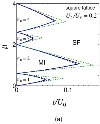
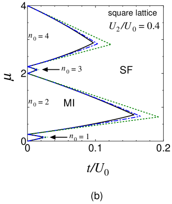
Figure 1: (Color online) Phase diagrams obtained by strong-coupling expansion for (a) $U_{2}/U_{0}=0.2$ and for (b) $U_{2}/U_{0}=0.4$ in the square lattice. The solid curves show the results up to third order in t. Results up to first order (second order) in $t$ are also shown by the green dashed (blue dot-dashed) curve.

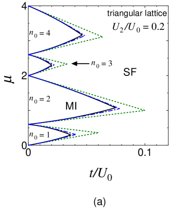
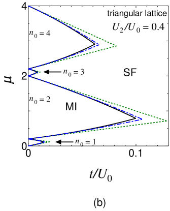
Figure 2: (Color online) Same plot as in Fig. 1 but for (a) $U_{2}/U_{0}=0.2$ and (b) $U_{2}/U_{0}=0.4$ in the triangular lattice.

Figures 1 and 2 show the phase diagram obtained from the strong-coupling expansion for the square lattice and for the triangular lattice, respectively. In both lattices, the MI phase for even-boson filling is considerably more stable against the SF phase than for odd-boson filling, which is consistent with QMC studies for the square lattice and MF studies. The area of the MI phase for even-boson (odd-boson) filling increases more (decreases more) for $U_{2}/U_{0}=0.4$ than for $U_{2}/U_{0}=0.2$. The convergence of the strong-coupling expansion from the first to the third order in $t$ is fairly good. We also find that higher-order terms mostly render the SF phase more stable against the MI phase because the area of the MI phase mostly becomes smaller for higher-order expansions, which is similar to the case of spinless Bose–Hubbard model.

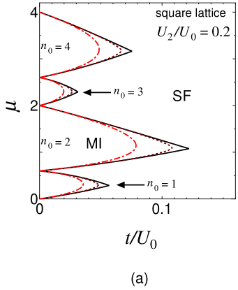
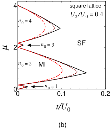
Figure 3: (Color Online) Phase diagrams for (a) $U_{2}/U_{0}=0.2$ and for (b) $U_{2}/U_{0}=0.4$ obtained by the strong-coupling expansion (solid curve) and its chemical-potential fitting (brown dashed curve) in the square lattice. The red dot-dashed curve shows the PMFA results.

The phase-boundary curve obtained by the strong-coupling expansion up to the third order in $t$ has a cusp at the peak of the Mott lobe. However, the chemical potential in infinite order in $t$ should follow a power-law scaling near $t_{\rm C}$, which is the value of $t$ at the tip of the Mott lobe. Following Ref. [12] to the spinless Bose–Hubbard model in 2D, we perform a chemical-potential fitting method which assumes

$$\mu=A(t)\pm B(t)(t_{\rm C}-t)^{z\nu}.$$ (10)

with a critical exponent $z\nu\simeq 2/3$. Here $A(t)\approx a+bt+ct^{2}+dt^{3}$ and $B(t)\approx\alpha+\beta t+\gamma t^{2}$ are the regular polynomial functions of $t$. By using our strong-coupling expansion up to the third order in $t$, we immediately determine $a$, $b$, $c$, and $d$ by setting $A(t)=[\mu^{\rm part}(t)+\mu^{\rm hole}(t)]/2$. In order to determine $\alpha$, $\beta$, $\gamma$, and $t_{\rm C}$ we compare the Taylor expansion of $t$ in $B(t)(t_{\rm C}-t)^{z\nu}$ with $[\mu^{\rm part}(t)-\mu^{\rm hole}(t)]/2$. Figures 3 and 4 compare the phase-boundary curves obtained by the third-order strong-coupling expansion with those obtained by the chemical-potential fitting in the square lattice and in the triangular lattice, respectively. The chemical-potential fitting makes the phase-boundary curves smooth and natural, as expected. The results obtained by the PMFA are also presented in both figures.

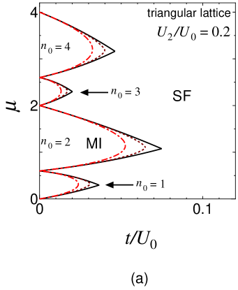
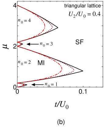
Figure 4: (Color online) Same plot as in Fig. 3 but for (a) $U_{2}/U_{0}=0.2$ and (b) $U_{2}/U_{0}=0.2$ in the triangular lattice.

For the square lattice, the QMC data show, for the $n_{0}=2$ Mott lobe, $t_{\rm C}/U_{0}\simeq 0.09(0.13)$ when $U_{2}/U_{0}=0.25(0.5)$ (as per our interpretation of Fig. 15 of Ref. [8]). Our third-order strong-coupling results and the chemical-potential fitting show $t_{\rm C}/U_{0}=0.132(0.187)$ when $U_{2}/U_{0}=0.25(0.5)$ and $t_{\rm C}/U_{0}=0.114(0.151)$ when $U_{2}/U_{0}=0.25(0.5)$, respectively. This shows that the chemical-potential fitting clearly improves the results obtained by the strong-coupling expansion up to third order in $t$. On the other hand, $t_{\rm C}/U_{0}=0.084(0.113)$ is obtained by the PMFA when $U_{2}/U_{0}=0.25(0.5)$. Hence the results obtained by QMC methods are in between those obtained by the chemical-potential fitting and PMFA, at least in the case of the square lattice where QMC has been performed. This seems to reflect the fact that the PMFA includes a part of the infinite-order terms in $t$ but neglects the quantum fluctuations that possibly stabilize the MI phase, whereas the chemical-potential fitting based on the strong-coupling expansion up to third order in $t$ includes the quantum fluctuations but does not directly include the higher-order terms in $t$ that possibly stabilize the SF phase.

Comparing the results obtained in the square lattice and those obtained in the triangular lattice, we find that $t_{\rm C}$ is roughly $6/4=3/2$ times greater in the square lattice than that in the triangular lattice, because of the difference between the number of nearest-neighbor sites $z$ [$z=4(6)$ in the square (triangular) lattice]. However, there seems to be no significant qualitative difference between the results obtained in the square lattice and those obtained in the triangular lattice. These results suggest that there the SF-MI transition has no significant dependence on the lattice structure.

4 Summary

In this paper, we present the strong-coupling expansion for the spin-1 Bose–Hubbard model for the square and triangular lattices. In both lattices, we confirm that for filling with an even number of bosons, the MI phase is considerably more stable against the SF phase than for filling with an odd number of bosons. We also fit the phase-boundary curves obtained by the strong-coupling expansion to the scaling form of the curves by using the chemical-potential fitting method. The fitting curves smooth and natural as expected, and the values of $t_{\rm C}$ are clearly improved.

Overall, there has been no essential difference in the phase boundary curves for the square and triangular lattices. This might be due to our assumption that the zeroth order in $t$ MI state is a nematic state. However, QMC study [8] of the square lattice indicates that the magnetic structure factor shows no trace of magnetic order anywhere in the phase diagram. Thus, in contrast to the usual antiferromagnetic spin systems, there might be no significant dependence on the lattice structure for spin-1 bosons in two or more dimensions.

4.1 Appendices

Appendix A Energies of Mott insulator and defect states in square and triangular lattices

By using $\Psi_{\rm even}$ and $\Psi_{\rm odd}$ [Eqs. (2) and (3)], the energy per site of the MI state in the square lattice is

$$\frac{E_{\rm square,MI,even}(n_{0})}{N} = \frac{U_{0}}{2}n_{0}(n_{0}-1)-U_{2}n_{0}-n_{0}\mu-\frac{z_{s}t^{2}}{3}\frac{n_{0}(n_{0}+3)}{U_{0}+2U_{2}},$$ (11)

$$\frac{E_{\rm square,MI,odd}(n_{0})}{N} = \frac{U_{0}}{2}n_{0}(n_{0}-1)-U_{2}(n_{0}-1)-n_{0}\mu$$ (12)

$$-\frac{1}{9}z_{s}t^{2}\Big{[}\frac{34}{25}\frac{(n_{0}+4)(n_{0}-1)}{U_{0}+4U_{2}}+\frac{4}{5}\frac{2n_{0}^{2}+6n_{0}+7}{U_{0}+U_{2}}$$

$$+\frac{(n_{0}+1)(n_{0}+2)}{U_{0}-2U_{2}}\Big{]}$$

up to the third order in $t$, and where $z_{s}=4$ is the number of nearest-neighbor sites in the square lattice. The corresponding MI-state energy in the triangular lattice is

$$\frac{E_{\rm triangular,MI,even}(n_{0})}{N}$$ (14)

$$= \frac{U_{0}}{2}n_{0}(n_{0}-1)-U_{2}n_{0}-n_{0}\mu-\frac{z_{t}t^{2}}{3}\frac{n_{0}(n_{0}+3)}{U_{0}+2U_{2}}-\frac{2}{9}z_{t}t^{3}\frac{n_{0}(n_{0}+3)(2n_{0}+3)}{(U_{0}+2U_{2})^{2}},$$

$$\frac{E_{\rm triangular,MI,odd}(n_{0})}{N}$$

$$= \frac{U_{0}}{2}n_{0}(n_{0}-1)-U_{2}(n_{0}-1)-n_{0}\mu$$

$$-\frac{1}{9}z_{t}t^{2}\Big{[}\frac{34}{25}\frac{(n_{0}-1)(n_{0}+4)}{U_{0}+4U_{2}}+\frac{4}{5}\frac{2n_{0}^{2}+6n_{0}+7}{U_{0}+U_{2}}+\frac{(n_{0}+1)(n_{0}+2)}{U_{0}-2U_{2}}\Big{]}$$

$$-\frac{2}{27}z_{t}t^{3}\Big{[}\frac{118}{125}\frac{(n_{0}-1)(n_{0}+4)(2n_{0}+3)}{(U_{0}+4U_{2})^{2}}+\frac{32}{25}\frac{(n_{0}-1)(n_{0}+4)(2n_{0}+3)}{(U_{0}+4U_{2})(U_{0}+U_{2})}$$

$$+\frac{4}{25}\frac{(n_{0}^{2}-1)(9n_{0}+1)+(n_{0}+2)(n_{0}+4)(9n_{0}+26)}{(U_{0}+U_{2})^{2}}$$

$$+\frac{8}{5}\frac{(n_{0}+1)(n_{0}+2)(2n_{0}+3)}{(U_{0}+U_{2})(U_{0}-2U_{2})}+\frac{(n_{0}+1)(n_{0}+2)(2n_{0}+3)}{(U_{0}-2U_{2})^{2}}\Big{]}$$

up to the third order in $t$, and where $z_{t}=6$ is the number of nearest-neighbor sites in the triangular lattice. Up to the second order in $t$, the expressions for the MI energy is the same for both lattices except for the difference between $z_{s}$ and $z_{t}$. However, in contrast to the square lattice, the third-order terms in $t$ exist for the triangular lattice.

The energies of the defect states can be obtained by using $\Psi^{\rm part}_{\rm even}$, $\Psi^{\rm hole}_{\rm even}$, $\Psi^{\rm part}_{\rm odd}$, and $\Psi^{\rm hole}_{\rm odd}$ [Eqs. (4)–(7)] up to the third order in $t$. For the square lattice, we obtain

$$E^{\rm part}_{\rm square,def,even}(n_{0})-E_{\rm square,MI,even}(n_{0})$$ (15)

$$= U_{0}n-\mu-z_{s}t\frac{n_{0}+3}{3}$$

$$-\frac{z_{s}(z_{s}-7)t^{2}}{9}\frac{n_{0}(n_{0}+3)}{U_{0}+2U_{2}}-\frac{z_{s}t^{2}n_{0}}{9}\Big{[}2\Big{(}\frac{n_{0}+5}{2U_{0}+3U_{2}}+\frac{n_{0}+3}{3U_{2}}\Big{)}+\frac{n_{0}+2}{2U_{0}}\Big{]}$$

$$-\frac{z_{s}t^{3}}{27}n_{0}(n_{0}+3)\Big{\{}(z_{s}-1)\Big{[}\frac{(2n_{0}+3)z_{s}-3(3n_{0}+8)}{(U_{0}+2U_{2})^{2}}$$

$$+\frac{2}{U_{0}+2U_{2}}\Big{(}2\frac{n_{0}+5}{2U_{0}+3U_{2}}+\frac{n_{0}+2}{2U_{0}}\Big{)}+\frac{4(n_{0}+3)}{3U_{2}(U_{0}+2U_{2})}\Big{]}$$

$$-z_{s}\Big{[}2\Big{(}\frac{n_{0}+5}{(2U_{0}+3U_{2})^{2}}+\frac{n_{0}+3}{(3U_{2})^{2}}\Big{)}+\frac{n_{0}+2}{(2U_{0})^{2}}\Big{]}+\frac{4}{3U_{2}}\Big{(}\frac{1}{5}\frac{n_{0}+5}{2U_{0}+3U_{2}}+\frac{n_{0}+2}{2U_{0}}\Big{)}\Big{\}},$$

$$E^{\rm hole}_{\rm square,def,even}(n_{0})-E_{\rm square,MI,even}(n_{0})$$ (16)

$$= -U_{0}(n_{0}-1)+2U_{2}+\mu-z_{s}t\frac{n_{0}}{3}$$

$$-\frac{z_{s}(z_{s}-7)t^{2}}{9}\frac{n_{0}(n_{0}+3)}{U_{0}+2U_{2}}-\frac{z_{s}t^{2}(n_{0}+3)}{9}\Big{[}2\Big{(}\frac{n_{0}-2}{2U_{0}+3U_{2}}+\frac{n_{0}}{3U_{2}}\Big{)}+\frac{n_{0}+1}{2U_{0}}\Big{]}$$

$$-\frac{z_{s}t^{3}}{27}n_{0}(n_{0}+3)\Big{\{}(z_{s}-1)\Big{[}\frac{(2n_{0}+3)z_{s}-3(3n_{0}+1)}{(U_{0}+2U_{2})^{2}}$$

$$+\frac{2}{U_{0}+2U_{2}}\Big{(}2\frac{n_{0}-2}{2U_{0}+3U_{2}}+\frac{n_{0}+1}{2U_{0}}\Big{)}+\frac{4n_{0}}{3U_{2}(U_{0}+2U_{2})}\Big{]}$$

$$-z_{s}\Big{[}2\Big{(}\frac{n_{0}-2}{(2U_{0}+3U_{2})^{2}}+\frac{n_{0}}{(3U_{2})^{2}}\Big{)}+\frac{n_{0}+1}{(2U_{0})^{2}}\Big{]}+\frac{4}{3U_{2}}\Big{(}\frac{1}{5}\frac{n_{0}-2}{2U_{0}+3U_{2}}+\frac{n_{0}+1}{2U_{0}}\Big{)}\Big{\}},$$

$$E^{\rm part}_{\rm square,def,odd}(n_{0})-E_{\rm square,MI,odd}(n_{0})$$ (17)

$$= U_{0}n_{0}-2U_{2}-z_{s}t\frac{n_{0}+1}{3}-\mu$$

$$-\frac{z_{s}(z_{s}-3)t^{2}}{9}(n_{0}+1)\Big{[}\frac{n_{0}+2}{U_{0}-2U_{2}}+\frac{4}{5}\frac{n_{0}-1}{U_{0}+U_{2}}\Big{]}$$

$$-\frac{z_{s}t^{2}}{9}(n_{0}+4)\Big{[}2\frac{n_{0}-1}{2U_{0}+3U_{2}}+\frac{n_{0}+2}{2U_{0}}-\frac{68}{25}\frac{n_{0}-1}{U_{0}+4U_{2}}-\frac{8}{5}\frac{n_{0}+2}{U_{0}+U_{2}}\Big{]}$$

$$-\frac{2}{45}z_{s}(2z_{s}+3)t^{2}\frac{(n_{0}+1)(n_{0}+4)}{3U_{2}}$$

$$-\frac{z_{s}(z_{s}-1)t^{3}}{27}\frac{(n_{0}+1)(n_{0}+2)}{(U_{0}-2U_{2})^{2}}\big{[}(2n_{0}+3)z_{s}-(5n_{0}+6)\big{]}$$

$$-\frac{4}{675}z_{s}(z_{s}-1)t^{3}\frac{n_{0}+1}{(U_{0}+U_{2})^{2}}\big{[}(n_{0}-1)(9n_{0}+1)z_{s}-2(17n_{0}^{2}+26n_{0}+32)\big{]}$$

$$-\frac{z_{s}(z_{s}-1)^{2}t^{3}}{27}\frac{n_{0}+1}{U_{0}+U_{2}}\Big{[}\frac{32}{25}\frac{(n_{0}-1)(n_{0}+4)}{U_{0}+4U_{2}}+\frac{8}{5}\frac{(n_{0}+2)(2n_{0}+3)}{U_{0}-2U_{2}}\Big{]}$$

$$-\frac{2}{27}z_{s}(z_{s}-1)t^{3}(n_{0}+1)(n_{0}+4)\Big{\{}\frac{n_{0}-1}{2U_{0}+3U_{2}}\Big{[}\frac{34}{25}\frac{1}{U_{0}+4U_{2}}+\frac{4}{5}\frac{1}{U_{0}+U_{2}}\Big{]}$$

$$+\frac{n_{0}+2}{2U_{0}}\Big{[}\frac{1}{U_{0}-2U_{2}}+\frac{4}{5}\frac{1}{U_{0}+U_{2}}\Big{]}+\frac{1}{3U_{2}}\Big{[}\frac{2}{25}(8z_{s}+9)\frac{n_{0}-1}{U_{0}+4U_{2}}+\frac{4}{5}z_{s}\frac{n_{0}+2}{U_{0}+U_{2}}\Big{]}\Big{\}}$$

$$-\frac{4}{135}z_{s}(2z_{s}+3)t^{3}\frac{(n_{0}+1)(n_{0}+4)}{3U_{2}}\Big{[}\frac{1}{5}\frac{n_{0}-1}{2U_{0}+3U_{2}}+\frac{n_{0}+2}{2U_{0}}\Big{]}$$

$$+\frac{2}{675}z_{s}t^{3}\frac{(n_{0}+1)(n_{0}+4)}{(3U_{2})^{2}}\big{[}2(n_{0}-11)z_{s}^{2}+9(3n_{0}+7)z_{s}-9(n_{0}+4)\big{]}$$

$$+\frac{z_{s}t^{3}}{27}(n_{0}+1)(n_{0}+4)\Big{[}\frac{68}{25}(z_{s}-1)\frac{n_{0}-1}{(U_{0}+4U_{2})^{2}}$$

$$+2z_{s}\frac{n_{0}-1}{(2U_{0}+3U_{2})^{2}}+z_{s}\frac{n_{0}+2}{(2U_{0})^{2}}\Big{]},$$

$$E^{\rm hole}_{\rm square,def,odd}(n_{0})-E_{\rm square,MI,odd}(n_{0})$$ (18)

$$= -U_{0}(n_{0}-1)-z_{s}t\frac{n_{0}+2}{3}+\mu$$

$$-\frac{z_{s}(z_{s}-3)t^{2}}{9}(n_{0}+2)\Big{[}\frac{n_{0}+1}{U_{0}-2U_{2}}+\frac{4}{5}\frac{n_{0}+4}{U_{0}+U_{2}}\Big{]}$$

$$-\frac{z_{s}t^{2}}{9}(n_{0}-1)\Big{[}2\frac{n_{0}+4}{2U_{0}+3U_{2}}+\frac{n_{0}+1}{2U_{0}}-\frac{68}{25}\frac{n_{0}+4}{U_{0}+4U_{2}}-\frac{8}{5}\frac{n_{0}+1}{U_{0}+U_{2}}\Big{]}$$

$$-\frac{2}{45}z_{s}(2z_{s}+3)t^{2}\frac{(n_{0}-1)(n_{0}+2)}{3U_{2}}$$

$$-\frac{z_{s}(z_{s}-1)t^{3}}{27}\frac{(n_{0}+1)(n_{0}+2)}{(U_{0}-2U_{2})^{2}}\big{[}(2n_{0}+3)z_{s}-(5n_{0}+9)\big{]}$$

$$-\frac{4}{675}z_{s}(z_{s}-1)t^{3}\frac{n_{0}+2}{(U_{0}+U_{2})^{2}}\big{[}(n_{0}+4)(9n_{0}+26)z_{s}-2(17n_{0}^{2}+76n_{0}+107)\big{]}$$

$$-\frac{z_{s}(z_{s}-1)^{2}t^{3}}{27}\frac{n_{0}+2}{U_{0}+U_{2}}\Big{[}\frac{32}{25}\frac{(n_{0}-1)(n_{0}+4)}{U_{0}+4U_{2}}+\frac{8}{5}\frac{(n_{0}+1)(2n_{0}+3)}{U_{0}-2U_{2}}\Big{]}$$

$$-\frac{2}{27}z_{s}(z_{s}-1)t^{3}(n_{0}-1)(n_{0}+2)\Big{\{}\frac{n_{0}+4}{2U_{0}+3U_{2}}\Big{[}\frac{34}{25}\frac{1}{U_{0}+4U_{2}}+\frac{4}{5}\frac{1}{U_{0}+U_{2}}\Big{]}$$

$$+\frac{n_{0}+1}{2U_{0}}\Big{[}\frac{1}{U_{0}-2U_{2}}+\frac{4}{5}\frac{1}{U_{0}+U_{2}}\Big{]}+\frac{1}{3U_{2}}\Big{[}\frac{2}{25}(8z_{s}+9)\frac{n_{0}+4}{U_{0}+4U_{2}}+\frac{4}{5}z_{s}\frac{n_{0}+1}{U_{0}+U_{2}}\Big{]}\Big{\}}$$

$$-\frac{4}{135}z_{s}(2z_{s}+3)t^{3}\frac{(n_{0}-1)(n_{0}+2)}{3U_{2}}\Big{[}\frac{1}{5}\frac{n_{0}+4}{2U_{0}+3U_{2}}+\frac{n_{0}+1}{2U_{0}}\Big{]}$$

$$+\frac{2}{675}z_{s}t^{3}\frac{(n_{0}-1)(n_{0}+2)}{(3U_{2})^{2}}\big{[}2(n_{0}+14)z_{s}^{2}+9(3n_{0}+2)z_{s}-9(n_{0}-1)\big{]}$$

$$+\frac{z_{s}t^{3}}{27}(n_{0}-1)(n_{0}+2)\Big{[}\frac{68}{25}(z_{s}-1)\frac{n_{0}+4}{(U_{0}+4U_{2})^{2}}$$

$$+2z_{s}\frac{n_{0}+4}{(2U_{0}+3U_{2})^{2}}+z_{s}\frac{n_{0}+1}{(2U_{0})^{2}}\Big{]}.$$

For the triangular lattice, we obtain

$$E^{\rm part}_{\rm triangular,def,even}(n_{0})-E_{\rm triangular,MI,even}(n_{0})$$ (19)

$$= U_{0}n-\mu-z_{t}t\frac{n_{0}+3}{3}$$

$$-\frac{z_{t}(z_{t}-7)t^{2}}{9}\frac{n_{0}(n_{0}+3)}{U_{0}+2U_{2}}-\frac{z_{t}t^{2}n_{0}}{9}\Big{[}2\Big{(}\frac{n_{0}+5}{2U_{0}+3U_{2}}+\frac{n_{0}+3}{3U_{2}}\Big{)}+\frac{n_{0}+2}{2U_{0}}\Big{]}$$

$$-\frac{z_{t}t^{3}}{27}n_{0}\Big{\{}\frac{n_{0}+3}{(U_{0}+2U_{2})^{2}}\big{[}(2n_{0}+3)z_{t}^{2}-2(4n_{0}+9)z_{t}-3(17n_{0}+32)\big{]}$$

$$-2\frac{n_{0}+5}{(2U_{0}+3U_{2})^{2}}\big{[}(n_{0}+3)z_{t}-2n_{0}\big{]}-\frac{n_{0}+2}{(2U_{0})^{2}}\big{[}(n_{0}+3)z_{t}-2n_{0}\big{]}-2(z_{t}-2)\frac{(n_{0}+3)^{2}}{(3U_{2})^{2}}$$

$$+2(z_{t}+1)\frac{n_{0}+3}{U_{0}+2U_{2}}\Big{[}2\frac{n_{0}+5}{2U_{0}+3U_{2}}+\frac{n_{0}+2}{2U_{0}}\Big{]}$$

$$+4\frac{n_{0}+3}{3U_{2}}\Big{[}\frac{(n_{0}+3)z+n_{0}-3}{U_{0}+2U_{2}}+\frac{1}{5}\frac{n_{0}+5}{2U_{0}+3U_{2}}+\frac{n_{0}+2}{2U_{0}}\Big{]}\Big{\}}$$

$$E^{\rm hole}_{\rm triangular,def,even}(n_{0})-E_{\rm triangular,MI,even}(n_{0})$$ (20)

$$= -U_{0}(n_{0}-1)+2U_{2}+\mu-z_{t}t\frac{n_{0}}{3}$$

$$-\frac{z_{t}(z_{t}-7)t^{2}}{9}\frac{n_{0}(n_{0}+3)}{U_{0}+2U_{2}}-\frac{z_{t}t^{2}(n_{0}+3)}{9}\Big{[}2\Big{(}\frac{n_{0}-2}{2U_{0}+3U_{2}}+\frac{n_{0}}{3U_{2}}\Big{)}+\frac{n_{0}+1}{2U_{0}}\Big{]}$$

$$-\frac{z_{t}t^{3}}{27}(n_{0}+3)\Big{\{}\frac{n_{0}}{(U_{0}+2U_{2})^{2}}\big{[}(2n_{0}+3)z_{t}^{2}-2(4n_{0}+3)z_{t}-3(17n_{0}+19)\big{]}$$

$$-2\frac{n_{0}-2}{(2U_{0}+3U_{2})^{2}}\big{[}n_{0}z_{t}-2(n_{0}+3)\big{]}-\frac{n_{0}+1}{(2U_{0})^{2}}\big{[}n_{0}z_{t}-2(n_{0}+3)\big{]}-2(z_{t}-2)\frac{n_{0}^{2}}{(3U_{2})^{2}}$$

$$+2(z_{t}+1)\frac{n_{0}}{U_{0}+2U_{2}}\Big{[}2\frac{n_{0}-2}{2U_{0}+3U_{2}}+\frac{n_{0}+1}{2U_{0}}\Big{]}$$

$$+4\frac{n_{0}}{3U_{2}}\Big{[}\frac{n_{0}z+n_{0}+6}{U_{0}+2U_{2}}+\frac{1}{5}\frac{n_{0}-2}{2U_{0}+3U_{2}}+\frac{n_{0}+1}{2U_{0}}\Big{]}\Big{\}}$$

$$E^{\rm part}_{\rm triangular,def,odd}(n_{0})-E_{\rm triangular,MI,odd}(n_{0})$$ (21)

$$= U_{0}n_{0}-2U_{2}-z_{t}t\frac{n_{0}+1}{3}-\mu$$

$$-\frac{z_{t}(z_{t}-3)t^{2}}{9}(n_{0}+1)\Big{[}\frac{n_{0}+2}{U_{0}-2U_{2}}+\frac{4}{5}\frac{n_{0}-1}{U_{0}+U_{2}}\Big{]}$$

$$-\frac{z_{t}t^{2}}{9}(n_{0}+4)\Big{[}2\frac{n_{0}-1}{2U_{0}+3U_{2}}+\frac{n_{0}+2}{2U_{0}}-\frac{68}{25}\frac{n_{0}-1}{U_{0}+4U_{2}}-\frac{8}{5}\frac{n_{0}+2}{U_{0}+U_{2}}\Big{]}$$

$$-\frac{2}{45}z_{t}(2z_{t}+3)t^{2}\frac{(n_{0}+1)(n_{0}+4)}{3U_{2}}$$

$$+\frac{2z_{t}t^{3}}{3375}\frac{(n_{0}-1)(n_{0}+4)}{(U_{0}+4U_{2})^{2}}\big{[}85(n_{0}+1)z_{t}+2(524n_{0}+701)\big{]}$$

$$+\frac{4}{675}\frac{z_{t}t^{3}}{(U_{0}+U_{2})^{2}}\Big{\{}(n_{0}^{2}-1)\big{[}-(9n_{0}+1)z_{t}^{2}+4(7n_{0}+3)z_{t}+8(11n_{0}+4)\big{]}$$

$$+(n_{0}+2)(n_{0}+4)\big{[}5(n_{0}+1)z_{t}+2(37n_{0}+88)\big{]}\Big{\}}$$

$$+\frac{z_{t}t^{3}}{27}\frac{(n_{0}+1)(n_{0}+2)}{(U_{0}-2U_{2})^{2}}\big{[}-(2n_{0}+3)z_{t}^{2}+2(3n_{0}+4)z_{t}+19n_{0}+26\big{]}$$

$$+\frac{2z_{t}t^{3}}{675}\frac{(n_{0}-1)(n_{0}+4)}{(2U_{0}+3U_{2})^{2}}\big{[}25(n_{0}+1)z_{t}-34(n_{0}-1)\big{]}$$

$$+\frac{z_{t}t^{3}}{27}\frac{(n_{0}+2)(n_{0}+4)}{(2U_{0})^{2}}\big{[}(n_{0}+1)z_{t}-2(n_{0}+2)\big{]}$$

$$+\frac{2z_{t}t^{3}}{675}\frac{(n_{0}+1)(n_{0}+4)}{(3U_{2})^{2}}\big{[}2(n_{0}-11)z_{t}^{2}+9(3n_{0}+7)z_{t}-27(n_{0}+4)\big{]}$$

$$-\frac{32z_{t}t^{3}}{675}\frac{(n_{0}-1)(n_{0}+4)}{(U_{0}+4U_{2})(U_{0}+U_{2})}\big{[}(n_{0}+1)z_{t}^{2}-2(n_{0}+1)z_{t}-(13n_{0}+19)\big{]}$$

$$-\frac{8}{135}z_{t}(z_{t}^{2}-2z_{t}-7)t^{3}\frac{(n_{0}+1)(n_{0}+2)(2n_{0}+3)}{(U_{0}+U_{2})(U_{0}-2U_{2})}-\frac{16z_{t}t^{3}}{135}\frac{(n_{0}-1)(n_{0}+2)(n_{0}+4)}{2U_{0}(2U_{0}+3U_{2})}$$

$$-\frac{68z_{t}t^{3}}{675}\frac{(n_{0}-1)(n_{0}+4)}{(2U_{0}+3U_{2})(U_{0}+4U_{2})}\big{[}(n_{0}+1)z_{t}+n_{0}+7\big{]}$$

$$-\frac{8}{135}z_{t}(z_{t}+1)t^{3}\frac{(n_{0}^{2}-1)(n_{0}+4)}{(2U_{0}+3U_{2})(U_{0}+U_{2})}-\frac{8z_{t}t^{3}}{135}\frac{(n_{0}+2)(n_{0}+4)}{2U_{0}(U_{0}+U_{2})}\big{[}(n_{0}+1)z_{t}+n_{0}+7\big{]}$$

$$-\frac{2}{27}z_{t}(z_{t}+1)t^{3}\frac{(n_{0}+1)(n_{0}+2)(n_{0}+4)}{2U_{0}(U_{0}-2U_{2})}-\frac{4}{675}z_{t}(8z_{t}^{2}+z_{t}+9)t^{3}\frac{(n_{0}^{2}-1)(n_{0}+4)}{3U_{2}(U_{0}+4U_{2})}$$

$$-\frac{8}{135}z_{t}^{2}(z_{t}-1)t^{3}\frac{(n_{0}+1)(n_{0}+2)(n_{0}+4)}{3U_{2}(U_{0}+U_{2})}-\frac{4}{675}z_{t}(2z_{t}+3)t^{3}\frac{(n_{0}^{2}-1)(n_{0}+4)}{3U_{2}(2U_{0}+3U_{2})}$$

$$-\frac{4}{135}z_{t}(2z_{t}+3)t^{3}\frac{(n_{0}+1)(n_{0}+2)(n_{0}+4)}{3U_{2}\cdot 2U_{0}}$$

$$E^{\rm hole}_{\rm triangular,def,odd}(n_{0})-E_{\rm triangular,MI,odd}(n_{0})$$ (22)

$$= -U_{0}(n_{0}-1)-z_{t}t\frac{n_{0}+2}{3}+\mu$$

$$-\frac{z_{t}(z_{t}-3)t^{2}}{9}(n_{0}+2)\Big{[}\frac{n_{0}+1}{U_{0}-2U_{2}}+\frac{4}{5}\frac{n_{0}+4}{U_{0}+U_{2}}\Big{]}$$

$$-\frac{z_{t}t^{2}}{9}(n_{0}-1)\Big{[}2\frac{n_{0}+4}{2U_{0}+3U_{2}}+\frac{n_{0}+1}{2U_{0}}-\frac{68}{25}\frac{n_{0}+4}{U_{0}+4U_{2}}-\frac{8}{5}\frac{n_{0}+1}{U_{0}+U_{2}}\Big{]}$$

$$-\frac{2}{45}z_{t}(2z_{t}+3)t^{2}\frac{(n_{0}-1)(n_{0}+2)}{3U_{2}}$$

$$+\frac{2z_{t}t^{3}}{3375}\frac{(n_{0}-1)(n_{0}+4)}{(U_{0}+4U_{2})^{2}}\big{[}85(n_{0}+2)z_{t}+2(524n_{0}+871)\big{]}$$

$$+\frac{4}{675}\frac{z_{t}t^{3}}{(U_{0}+U_{2})^{2}}\Big{\{}(n_{0}+2)(n_{0}+4)\big{[}-(9n_{0}+26)z_{t}^{2}+4(7n_{0}+18)z_{t}+8(11n_{0}+29)\big{]}$$

$$+(n_{0}^{2}-1)\big{[}5(n_{0}+2)z_{t}+2(37n_{0}+23)\big{]}\Big{\}}$$

$$+\frac{z_{t}t^{3}}{27}\frac{(n_{0}+1)(n_{0}+2)}{(U_{0}-2U_{2})^{2}}\big{[}-(2n_{0}+3)z_{t}^{2}+2(3n_{0}+5)z_{t}+19n_{0}+31\big{]}$$

$$+\frac{2z_{t}t^{3}}{675}\frac{(n_{0}-1)(n_{0}+4)}{(2U_{0}+3U_{2})^{2}}\big{[}25(n_{0}+2)z_{t}-34(n_{0}+4)\big{]}$$

$$+\frac{z_{t}t^{3}}{27}\frac{n_{0}^{2}-1}{(2U_{0})^{2}}\big{[}(n_{0}+2)z_{t}-2(n_{0}+1)\big{]}$$

$$+\frac{2z_{t}t^{3}}{675}\frac{(n_{0}-1)(n_{0}+2)}{(3U_{2})^{2}}\big{[}2(n_{0}+14)z_{t}^{2}+9(3n_{0}+2)z_{t}-27(n_{0}-1)\big{]}$$

$$-\frac{32z_{t}t^{3}}{675}\frac{(n_{0}-1)(n_{0}+4)}{(U_{0}+4U_{2})(U_{0}+U_{2})}\big{[}(n_{0}+2)z_{t}^{2}-2(n_{0}+2)z_{t}-(13n_{0}+20)\big{]}$$

$$-\frac{8}{135}z_{t}(z_{t}^{2}-2z_{t}-7)t^{3}\frac{(n_{0}+1)(n_{0}+2)(2n_{0}+3)}{(U_{0}+U_{2})(U_{0}-2U_{2})}-\frac{16z_{t}t^{3}}{135}\frac{(n_{0}^{2}-1)(n_{0}+4)}{2U_{0}(2U_{0}+3U_{2})}$$

$$-\frac{68z_{t}t^{3}}{675}\frac{(n_{0}-1)(n_{0}+4)}{(2U_{0}+3U_{2})(U_{0}+4U_{2})}\big{[}(n_{0}+2)z_{t}+n_{0}-4\big{]}$$

$$-\frac{8}{135}z_{t}(z_{t}+1)t^{3}\frac{(n_{0}-1)(n_{0}+2)(n_{0}+4)}{(2U_{0}+3U_{2})(U_{0}+U_{2})}-\frac{8z_{t}t^{3}}{135}\frac{n_{0}^{2}-1}{2U_{0}(U_{0}+U_{2})}\big{[}(n_{0}+2)z_{t}+n_{0}-4\big{]}$$

$$-\frac{2}{27}z_{t}(z_{t}+1)t^{3}\frac{(n_{0}^{2}-1)(n_{0}+2)}{2U_{0}(U_{0}-2U_{2})}-\frac{4}{675}z_{t}(8z_{t}^{2}+z_{t}+9)t^{3}\frac{(n_{0}-1)(n_{0}+2)(n_{0}+4)}{3U_{2}(U_{0}+4U_{2})}$$

$$-\frac{8}{135}z_{t}^{2}(z_{t}-1)t^{3}\frac{(n_{0}^{2}-1)(n_{0}+2)}{3U_{2}(U_{0}+U_{2})}-\frac{4}{675}z_{t}(2z_{t}+3)t^{3}\frac{(n_{0}-1)(n_{0}+2)(n_{0}+4)}{3U_{2}(2U_{0}+3U_{2})}$$

$$-\frac{4}{135}z_{t}(2z_{t}+3)t^{3}\frac{(n_{0}^{2}-1)(n_{0}+2)}{3U_{2}\cdot 2U_{0}}$$

As for the MI energy, the expressions for the MI energy up to the second order in $t$ are the same for both lattices except for the difference between $z_{s}$ and $z_{t}$ but the third-order terms in $t$ are different from each lattice. This difference between the third-order terms originates from particles or holes that can (cannot) return to their original site through three hopping processes in the triangular (square) lattice.

References

References

- [1] Stamper-Kurn D M and Ueda M 2013 Rev. Mod. Phys. 85 1191; Lewenstein M, Sanpera A and Ahufinger V 2012 Ultracold Atoms in Optical Lattices: Simulating Quantum Many-Body Systems (Oxford Univ. Pr.)
- [2] Katsura H and Tasaki H 2013 Phys. Rev. Lett. 110 130405
- [3] Tsuchiya S, Kurihara S and Kimura T 2004 Phys. Rev. A 70 043628
- [4] Rizzi M, Rossini D, De Chiara G, Montangero S and Fazio R 2005 Phys. Rev. Lett. 95 240404
- [5] Batrouni G G, Rousseau V G and Scalettar R T 2009 Phys. Rev. Lett. 102 140402
- [6] Apaja V and Syljuåsen O F 2006 Phys. Rev. A 74 035601
- [7] Toga Y, Tsuchiura H, Yamashita M, Inaba K and Yokoyama H 2012 J. Phys. Soc. Jpn. 81 063001
- [8] de Forges de Parny L, Hébert F, Rousseau V G and Batrouni G G arXiv:1306.5515
- [9] Kimura T, Tsuchiya S and Kurihara S 2005 Phys. Rev. Lett. 94 110403
- [10] Krutitsky K V and Graham R 2004 Phys. Rev. A 70 063610
- [11] Krutitsky K V, Timmer M and Graham R 2005 Phys. Rev. A 71 033623
- [12] Freericks J K and Monien H 1996 Phys. Rev. B 53 2691; Freericks J K and Monien H 1994 Europhys. Lett. 26, 545
- [13] Freericks J K, Krishnamurthy H R, Kato Y, Kawashima N and Trivedi N 2009 Phys. Rev. A 79 053631
- [14] Iskin M and Freericks J K 209 Phys. Rev. A 79 053634
- [15] Hen I, Iskin M and Rigol M 2010 Phys. Rev. B 81 064503
- [16] Iskin M 2010 Phys. Rev. A 82 033630
- [17] Kimura T 2013 Phys. Rev. A 87 043624