Goos-Hänchen-like shift of three-level matter wave incident on Raman beams

Abstract

When a three-level atomic wavepacket is obliquely incident on a ”medium slab” consisting of two far-detuned laser beams, there exists lateral shift between reflection and incident points at the surface of a ”medium slab”, analogous to optical Goos-Hänchen effect. We evaluate lateral shifts for reflected and transmitted waves via expansion of reflection and transmission coefficients, in contrast to the stationary phase method. Results show that lateral shifts can be either positive or negative dependent on the incident angle and the atomic internal state. Interestingly, a giant lateral shift of transmitted wave with high transmission probability is observed, which is helpful to observe such lateral shifts experimentally. Different from the two-level atomic wave case, we find that quantum interference between different atomic states plays crucial role on the transmission intensity and corresponding lateral shifts.

¹ Key Laboratory of Photo-electronic, Telecommunication of Jiangxi Province, Jiangxi Normal University, Nanchang, 330022, China
² Center for Engineered Quantum System, School of Mathematics and Physics, University of Queensland, St Lucia, 4072, Qld, Australia ^∗ duanzhenglu@jxnu.edu.cn

(020.1335) Atom optics; (260.3160) Interference;(240.7040) Tunneling.

1 Introduction

The exit point of a light beam totally reflected by a surface separating two different refractive index media will experience a lateral displacement corresponding to the incident point. This phenomenon is called the Goos-Hänchen effect [1, 2] and was first experimentally demonstrated by Goos and Hänchen in 1947. However,as early as 270 years ago, Newton intuitively conjectured it via using light ray reflection from the surface of a mirror [3]. Soon after Goos and Hänchen’s experiment, Artmann theoretically evaluated the lateral displacement using stationary phase method starting from Maxwell equations [4]. In 1964, Renard applied energy flux conservation to explain Goos-Hänchen effect [5].

Recently its consideration has been extended to cases involving multilayered structures [6], left-hand material [7], absorptive, amplified and nonlinear media [8]. In fact, the total reflection conditions are not necessary for the lateral shift as long as there are appropriate phase changes in the plane wave component, resulting in the transmitted beam also experiencing such shift [9]. Furthermore, existence of large and negative Goos-Hänchen shift also has been investigated in some circumstances [10, 11, 12]. Apart from fundamental research, the Goos-Hänchen effect has application in surface plasmon resonance sensor [13], near-field scanning optical microscopy [14] and optical waveguide switch [15].

Since the Goos-Hänchen effect comes from wave interference, one can expect it to also take place in other physical systems, such as acoustic waves, plasma and matter waves. Refs [16, 17, 18] investigate lateral shifts of acoustic wave theoretically and experimentally; while as early as 1960, Hora derived an expression for Goos-Hänchen shift experienced by a beam of quantum particles [19]. Since then the Goos-Hänchen effect has been investigated in electron [20, 21] and neutron [22, 23] cases, theoretically and experimentally.

Thanks to the rapid development of laser cooling and trapping technology, one can manipulate the ensemble of ultracold atoms for fundamental and applied investigation under straightforward laboratory conditions, for example, atom guiding [24], reflecting [25] and diffracting [26], resulting in these advancements in the field of the atom optics.

The ultracold atomic beam transmited through a laser field [27] or a cavity in one-dimensional (1D) constitution [28] has been investigated. When the atomic beam is obliquely incident on a potential barrier, Goos-Hänchen-like effect may emerge. Unlike light waves in traditional optics, matter waves in atom optics can behave differently, for the atom has internal electronic structures and matter waves of atoms are coupled vector waves in the light-induced ”medium”. We have found that there are large positive and negative lateral shifts for two-level ultracold two-dimensional (2D) atomic wavepacket in our previous work [29]. This work investigates what happens when a three-dimensional (3D) $\Lambda$-type three-level ultracold atomic wavepacket obliquely impinges on Raman laser beams.

This paper is organized as follows: In Sec. II, we firstly construct an atomic optics model describing a three-level atomic wavepacket impinging on pairs of super-Gaussian Raman laser beams acting as a ”medium slab”. And then In Sec. III, we obtain the Goos-Hänchen-like lateral shifts of reflected and transmitted waves by expansion of reflection and transmission coefficients. Sec. IV gives the numerical results for lateral shifts under blue and red detuned situations and the effect of quantum interference on the lateral shift of transmitted waves. Finally, in Sec. IV we conclude this paper.

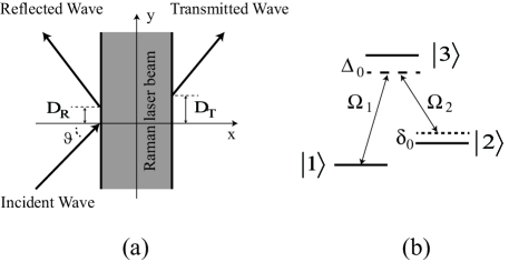
Figure 1: (a) Schematic of lateral shift when a three-level atomic wavepacket oblique incident on a Raman laser beams. (b) Energy level structure of atom.

2 Model

In this work we consider a 3D cold $\Lambda$-type three-level atomic wavepacket obliquely impinging on a pair of flat top laser fields with a width $L$ (Shown in Fig. 1), which could be realized with a super-Gaussian laser field with a high order [30, 31, 32]. The $\Lambda$-type three-level scheme can be realized, for example, by two $6S_{1/2}$ hyperfine ground states $F=3$ and $F=4$ (hypefine splitting = 9.19 GHz) of ¹³³Cs atoms, which are labeled as $|1\rangle$ and $|2\rangle$, respectively. The $F^{{}^{\prime}}=4$ hyperfine level of the electronically excited state, $6P_{3/2}$, forms the intermediate state, $|3\rangle$. The atom interacts with two laser beams with frequencies $\omega_{L1}$ and $\omega_{L2}$ and they are detuned from $|1\rangle\rightarrow|3\rangle$ and $|2\rangle\rightarrow|3\rangle$ transitions by $\Delta$. The Schrödinger equations governing this system are given by

$$i\hbar\frac{\partial}{\partial t}\Psi_{1}\left(\mathbf{r},t\right) =-\frac{\hbar^{2}}{2m}\nabla^{2}\Psi_{1}\left(\mathbf{r},t\right)-\frac{\hbar}{2}\Omega_{1}\left(x\right)e^{-ik_{L1}y}\Psi_{3}\left(\mathbf{r},t\right)$$ (1)

$$i\hbar\frac{\partial}{\partial t}\,\Psi_{2}\left(\mathbf{r},t\right) =-\frac{\hbar^{2}}{2m}\nabla^{2}\Psi_{2}\left(\mathbf{r},t\right)-\hbar\delta_{0}\psi_{2}\left(\mathbf{r},t\right)$$

$$-\frac{\hbar}{2}\Omega_{2}\left(x\right)e^{-ik_{L2}y}\Psi_{3}\left(\mathbf{r},t\right)$$ (2)

$$i\hbar\frac{\partial}{\partial t}\,\Psi_{3}\left(\mathbf{r},t\right) =-\frac{\hbar^{2}}{2m}\nabla^{2}\Psi_{3}\left(\mathbf{r},t\right)-\hbar\left(\Delta_{0}+\frac{i\gamma}{2}\right)\Psi_{3}\left(\mathbf{r},t\right)$$

$$-\frac{\hbar}{2}\Omega_{1}\left(x\right)e^{ik_{L1}y}\Psi_{1}\left(\mathbf{r},t\right)-\frac{\hbar}{2}\Omega_{2}\left(x\right)e^{ik_{L2}y}\Psi_{2}\left(\mathbf{r},t\right)$$ (3)

In Eqs. (1a)–(1c) we have defined $m$ as the atomic mass, $\nabla^{2}=\partial^{2}/\partial x^{2}+\partial^{2}/\partial y^{2}+\partial^{2}/\partial z^{2}$, $\Delta_{0}=\omega_{L1}-\omega_{3}$ as the single-photon detuning and $\delta_{0}=\omega_{L1}-\omega_{L2}-\omega_{2}$ as the two-photon detuning, $\gamma$ as the decay rate of excited state $|3\rangle$.

We assume that both laser beams have the same beam profile:

$$\Omega_{1,2}\left(x\right)=\left\{\begin{array}[]{lcl}\Omega_{1,2}&,&0\leq x\leq L\\ 0&,&\text{\ }x<0,x>L\end{array}\right..$$ (4)

Owing to the Rabi frequencies $\Omega_{1,2}$ being $y$ and $z$ independent, we eliminate $y$ and $z$ components of the wavefunction through Fourier transformation

$$\Psi_{1}\left(\mathbf{r},t\right) =\int dk_{y}dk_{z}\psi_{1}\left(x,t\right)e^{ik_{y}y-i\hbar\left(k_{y}^{2}+k_{z}^{2}\right)t/2m},$$ (5)

$$\Psi_{2}\left(\mathbf{r},t\right) =\int dk_{y}dk_{z}\psi_{2}\left(x,t\right)e^{i\left(k_{y}+k_{L1}+k_{L2}\right)y-i\hbar\left(k_{y}^{2}+k_{z}^{2}\right)t/2m},$$ (6)

$$\Psi_{3}\left(\mathbf{r},t\right) =\int dk_{y}dk_{z}\psi_{3}\left(x,t\right)e^{i\left(k_{y}+k_{L1}\right)y-i\hbar\left(k_{y}^{2}+k_{z}^{2}\right)t/2m}.$$ (7)

By substituting Eqs. (3a)–(3c) into Eqs. (1a)–(1c) we obtain coupled 1D Schrödinger equations

$$i\hbar\frac{\partial}{\partial t}\,\psi\left(x,t\right)=\left(-\frac{\hbar^{2}}{2m}\frac{\partial^{2}}{\partial x^{2}}\hat{I}+\hat{V}\right)\psi\left(x,t\right)$$ (8)

where $\psi\left(x,t\right)=\left(\psi_{1}\left(x,t\right),\psi_{2}\left(x,t\right),\psi_{3}\left(x,t\right)\right)^{T}$ is a three component vector wavefunction, $\hat{I}$ is a $3\times 3$ unit matrix, and $\hat{V}$ is the potential as matrix form by

$$\hat{V}=-\frac{\hbar}{2}\left(\begin{array}[]{ccc}0&0&\Omega_{1}\\ 0&2\delta&\Omega_{2}\\ \Omega_{1}&\Omega_{2}&2\Delta\end{array}\right),$$ (9)

here we have defined effective single-photon detuning and effective two-photon detuning, respectively, are:

$$\Delta =\Delta_{0}-\frac{\hbar}{2m}\left(2k_{L1}k_{y}+k_{L1}^{2}\right)+\frac{i}{2}\gamma$$ (10)

$$\delta =\delta_{0}+\frac{\hbar}{2m}\allowbreak k_{y}^{2}-\frac{\hbar}{2m}\allowbreak\left(k_{L1}+k_{L2}+k_{y}\right)^{2}$$ (11)

We consider effective two-photon resonance situation, i.e., $\delta=0$. In this case, the eigenvalues of the matrix $V$ are $V_{0}=0$ and $V_{\pm}=-\hbar\left(\Delta\mp\tilde{\Delta}\right)/2$ with $\tilde{\Delta}=\sqrt{\Delta^{2}+\Omega_{1}^{2}+\Omega_{2}^{2}}$, and the corresponding transformation matrix is

$$U=\left(\begin{array}[]{ccc}\frac{\Omega_{1}}{\Delta-\tilde{\Delta}}&-\frac{\Omega_{2}}{\Omega_{1}}&\frac{\Omega_{1}}{\Delta+\tilde{\Delta}}\\ \frac{\Omega_{2}}{\Delta-\tilde{\Delta}}&1&\frac{\Omega_{2}}{\Delta+\tilde{\Delta}}\\ 1&0&1\end{array}\right)$$ (12)

3 Lateral shifts of transmitted and reflected Wavepackets

The wave packet cannot be described by a stationary wave function, we therefore address the dynamic evolution of cold atom wavepacket to evaluate the lateral shift. Here we first take the atom wavepacket in state $|1\rangle$ for an example to illustrate how to obtain the lateral shift. The wave function of incident wavepacket can be described as:

$$\psi_{in}\left(\mathbf{r},t\right)=\int f\left(\mathbf{k}\right)\exp\left(i\mathbf{k}\cdot\mathbf{r}-iE/\hbar t\right)d\mathbf{k}$$ (13)

where $f\left(\mathbf{k}\right)$ $\left(2W^{2}/\pi\right)^{3/4}\exp\left(-W^{2}\left(\mathbf{k-k}_{0}\right)^{2}\right)$ is 3D momentum distribution function around the center wave vector $\mathbf{k}_{0}=\left(k_{x0},k_{y0},,0\right)$ at initial time. For a 3D wavepacket, the three components of wave vector $\mathbf{k}$ are decoupled.

After integration, we have

$$\psi_{in}\left(\mathbf{r},t\right)=\left(\frac{1}{2\pi A^{2}}\right)^{3/4}\exp\left(-\frac{\left(\mathbf{r}-\hbar\mathbf{k}_{0}t/m\right)^{2}}{4A^{2}}+i\mathbf{k}_{0}\left(\mathbf{r}-\frac{\hbar\mathbf{k}_{0}}{2m}t\right)\right)$$ (14)

where $A=W\sqrt{1+i\hbar t/\left(2mW^{2}\right)}$.

The transmitted wave packet can be expressed in a similar way:

$$\psi_{t}\left(\mathbf{r},t\right)=\int Tf\left(\mathbf{k}\right)\exp\left(i\mathbf{k}\cdot\mathbf{r}-iE/\hbar t\right)d\mathbf{k}$$ (15)

where $T$ is the transmission coefficient, whose expression is given in the Appendix.

For a wide momentum distribution $f\left(\mathbf{k}\right)$ of incident wave, the reflected and transmitted waves will be badly distorted, or even split, especially around the dip or pole of reflection and transmission probability, because the ”medium slab” severely modifies the reflected and transmitted momentum distribution far from a gaussian type. In this case, conventional definition of the lateral displacement in [4] would be invalid. This situation has been addressed in [11, 33]. To avoid severe distortion of the reflected and transmitted waves, a narrow momentum distribution of incident wave is required. To this end, here we assume $W$ is sufficiently large that reflection coefficient $T$ is approximately a constant in the region $k_{0}\pm 1/W$. With the assumption we can expand the transmission coefficient $T$ around $\left(k_{x0},k_{y0},0\right)$ up to linear term $T=\left|T\left(\mathbf{k}_{0}\right)\right|\exp\left(\left(\mathbf{\lambda}+i\mathbf{\phi}^{{}^{\prime}}\right)\left(\mathbf{k}-\mathbf{k}_{0}\right)\right)$, where $\mathbf{\lambda}=\left(d\left(\ln\left|T\right|\right)/dk_{x}|_{k_{x0}},d\left(\ln\left|T\right|\right)/dk_{y}|_{k_{y0}},0\right)$ and $\mathbf{\phi}=\left(d\phi/dk_{x}|_{k_{x0}},d\phi/dk_{y}|_{k_{y0}},0\right)$. Hence, the transmitting wave can be expressed as

$$\psi_{t}\left(\mathbf{r},t\right) =\left(\frac{1}{2\pi A^{2}}\right)^{3/4}\left|T\left(\mathbf{k}_{0}\right)\right|\exp\left(\frac{\mathbf{\lambda}^{2}}{4W^{2}}\right)$$

$$\times\exp\left(-\frac{\left(\mathbf{r}^{\prime}-\hbar\mathbf{k}_{0}^{\prime}t/m\right)^{2}}{4A^{2}}+i\mathbf{k}_{0}\left(\mathbf{r}^{\prime}-\mathbf{\phi}^{{}^{\prime}}-\frac{\hbar\mathbf{k}_{0}}{2m}t\right)\right)$$ (16)

where the wave center wave vector $\mathbf{k}_{0}^{\prime}\mathbf{=k}_{0}+\mathbf{\lambda/}\left(2W^{2}\right)$ and wave packet center $\mathbf{r}^{\prime}\mathbf{=r}+\mathbf{\phi}^{{}^{\prime}}$.

When the center of the transmitted wavepacket traverses through the right boundary, from (16), it follows that

$$y+\phi_{ty}^{{}^{\prime}}-\hbar k_{y0}^{\prime}t/m =0$$ (17)

$$L+\phi_{tx}^{{}^{\prime}}-\hbar k_{x0}^{\prime}t/m =0$$ (18)

And the shift along $y$ direction is

$$D_{t}=\frac{k_{y0}^{\prime}}{k_{x0}^{\prime}}\left(L+\phi_{tx}^{{}^{\prime}}\right)-\phi_{ty}^{{}^{\prime}}$$ (19)

Considering a large width of the wave packet, $\mathbf{\lambda/}\left(2W^{2}\right)\approx 0$, Eq. (19) becomes

$$D_{t}=\frac{k_{y0}}{k_{x0}}\left(L+\phi_{tx}^{{}^{\prime}}\right)-\phi_{ty}^{{}^{\prime}}$$ (20)

which is the same as that in [29].

Using the same procedure, we have the lateral shift for the reflected atomic packet

$$D_{r}=\frac{k_{y0}}{k_{x0}}\phi_{rx}^{{}^{\prime}}-\phi_{ry}^{{}^{\prime}}$$ (21)

Equations (20) and (21) show that we must find the transmission and reflection coefficients of the atomic wavepacket to determine the corresponding lateral shifts. The detailed derivation can be found in the Appendix.

4 Numerical results and discussion

In this section we numerically study the lateral shifts using Eqs. (20) and (21). In the following we take $k_{x0}=k_{0}\cos\left(\theta\right)$ and $k_{y0}=k_{0}\sin\left(\theta\right)$, and correspondingly,

$$\frac{\partial}{\partial k_{x0}} = \left(\cos\left(\theta\right)\frac{\partial}{\partial k_{0}}-\sin\left(\theta\right)\frac{\partial}{k_{0}\partial\theta}\right)$$ (22)

$$\frac{\partial}{\partial k_{y0}} = \left(\sin\left(\theta\right)\frac{\partial}{\partial k_{0}}+\cos\left(\theta\right)\frac{\partial}{k_{0}\partial\theta}\right)$$ (23)

where $k_{0}$ is the magnitude of the incident wave vector and $\theta$ is the incident angle of atomic wave packet. In such a circumstance the lateral shift of the reflected and transmitted waves are rewritten as

$$D_{r,t}=-\frac{1}{\cos\left(\theta\right)k_{0}}\frac{\partial\phi_{r,t}}{\partial\theta}$$ (24)

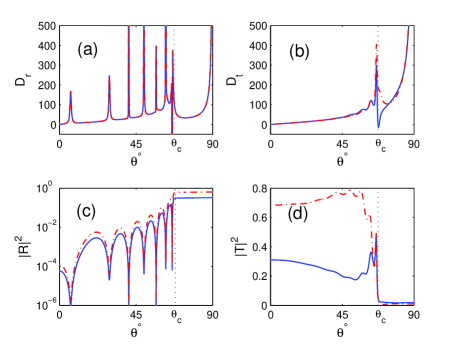
Figure 2: The lateral shift (upper panel) and reflection(transmission) probability (Lower panel) as a function of incident angle for atomic waves in state $\left|1\right\rangle$(solid line) and state $\left|2\right\rangle$(dash-dotted line). The incident atomic wave is in state $\left|1\right\rangle$ through the blue-detuned laser beams with different Rabi frequencies. Other parameters are: $L=30$, $\gamma=0.1$, $\Omega_{1}=2.5$, $\Omega_{2}=3.5$, $k_{0}=0.8$, $k_{L}=0.1$.

The variables and parameters in all the figures are dimensionless.

We first consider the blue detuned case with single-photon detuning $\Delta_{0}=100$. (Here we should stress that, even $\Delta_{0}\gg\Omega_{1},\Omega_{2}$ and $\gamma$, adiabatic elimination of excited state $\left|3\right\rangle$ may lead to loss of many important features of tunneling and Goos-Hänchen-like lateral shifts of atomic wave with internal structure [34].) At this case, the atomic states $\left|{1}\right\rangle$ and $\left|{2}\right\rangle$ can be approximately expressed as with dressed-state bases (29) and (30):

$$\left|1\right\rangle \approx \frac{\Omega_{1}\left|+\right\rangle+\Omega_{2}\left|0\right\rangle}{\sqrt{\Omega_{1}^{2}+\Omega_{2}^{2}}}$$ (25)

$$\left|2\right\rangle \approx \frac{\Omega_{2}\left|+\right\rangle-\Omega_{1}\left|0\right\rangle}{\sqrt{\Omega_{1}^{2}+\Omega_{2}^{2}}}$$ (26)

$$\left|3\right\rangle \approx \left|-\right\rangle$$ (27)

It can be seen that the scattering properties of atomic waves in states $\left|1\right\rangle$ and $\left|2\right\rangle$ are mainly determined by $\left|+\right\rangle$ and $\left|0\right\rangle$ modes. Apparently, if the initial states of the atomic wavepacket is in states $\left|1\right\rangle$ or $\left|2\right\rangle$, the atomic wavepacket will mainly ”see” a potential barrier since $\mathbf{Re}\left(V_{+}\right)>0$. Hence we can define a critical angle as $\theta_{c}\equiv\cos^{-1}\left(\sqrt{2m\mathbf{Re}\left(V_{+}\right)/\hbar^{2}k_{x0}^{2}}\right)$, at which the normal component of kinetic energy of the incident atomic wave equals the height of the potential barrier. If the incident angle of the atomic wave is greater than the critical angle, the atomic wave tunnels through the barrier; otherwise it passes over the barrier.

Figure 2 shows lateral shifts of reflected and transmitted waves with the incident atomic wave in state $\left|1\right\rangle$ and $\Omega_{1}\neq\Omega_{2}$. It can be found that the behavior of reflected and transmitted waves are quite different in the region $\theta>\theta_{c}$ and $\theta_{c}>\theta>0$. For $\theta_{c}>\theta>0$, the normal component of kinetic energy of incident atomic wave is greater than the height of barrier. As a result, the reflected and transmitted waves oscillate [Figs. 2(c) and 2(d)] and the lateral shifts exhibit giant peaks at each resonance [Figs. 2(a) and 2(b)]. For $\theta>\theta_{c}$, there are no peaks on the curves of lateral shifts. In fact, similar phenomena have been observed in [29]. One interesting thing is that, the lateral shifts of reflected waves in states $\left|1\right\rangle$ and $\left|2\right\rangle$ are equal, while the transmitted ones are not. This can be understood that, based on Eqs. (25) and (26), only $\left|+\right\rangle$ mode contributes to the reflected wave, consequently the reflected waves in state $\left|1\right\rangle$ and $\left|2\right\rangle$ acquire the same phase shift after leaving the reflection surface and the corresponding lateral shifts are equal although they have different reflection probabilities [Fig. 2(c)]. While in the transmission case, states $\left|1\right\rangle$ and $\left|2\right\rangle$ are superpositions of $\left|+\right\rangle$ mode and $\left|0\right\rangle$ mode with different signs, which leads to constructive or destructive quantum interference. The consequence is that the transmission intensities of the transmitted waves in state $\left|1\right\rangle$ and $\left|2\right\rangle$ have opposite trends when the incident angle is varied [Fig. 2(d)]. Also, the lateral shifts are different [Fig. 2(b)] for different states.

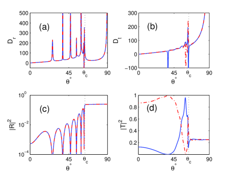
Figure 3: The lateral shift (upper panel) and reflection(transmission) probability (Lower panel) as a function of incident angle for atomic waves in state $\left|1\right\rangle$(solid line) and state $\left|2\right\rangle$(dash-dotted line). The incident atomic wave is in state $\left|1\right\rangle$ through the blue-detuned laser beams with equal Rabi frequencies. Other parameters are the same with figure 2.

Now we pay attention to the situation with $\Omega_{1}=\Omega_{2}=3.5$. Again, the incident atomic wave is set in state $\left|1\right\rangle$. Figures 3(a) and 3(b) show the lateral shift of reflected and transmitted waves in states $\left|1\right\rangle$ and $\left|2\right\rangle$ as a function of the incident angle, respectively. We observe multiple peaks and dips on the lateral shift curves of the reflected and transmitted waves, resulting from the resonance scattering. One most interesting things is that the reflection intensities of atomic waves in states $\left|1\right\rangle$ and $\left|2\right\rangle$ are the same, shown in [Fig. 3(c)]. Eqs. (25) and (26) are able to explain this phenomenon, given $\Omega_{1}=\Omega_{2}$, $\left|+\right\rangle$ mode equally contributes to the reflected waves in states $\left|1\right\rangle$ and $\left|2\right\rangle$. Another significant difference is that the lateral shift of transmitted wave in state $\left|1\right\rangle$ exhibits a giant negative peak at $\theta\approx 38^{\circ}$ [Fig. 3(b)]. This corresponds to a nearly vanishing transmission [Fig. 3(d)], which results from the nearly perfect quantum destructive interference, instead of resonance scattering.

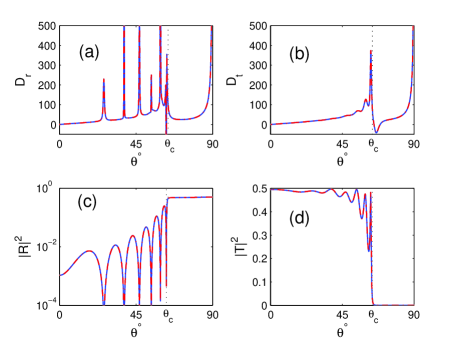
Figure 4: The lateral shift (upper panel) and reflection(transmission) probability (Lower panel) as a function of incident angle for atomic waves in state $\left|1\right\rangle$(solid line) and state $\left|2\right\rangle$(dash-dotted line). The incident atomic wave is in state $\left(\left|1\right\rangle+\left|2\right\rangle\right)/\sqrt{2}$ through the blue-detuned laser beams with equal Rabi frequencies. Other parameters are the same with figure 3.

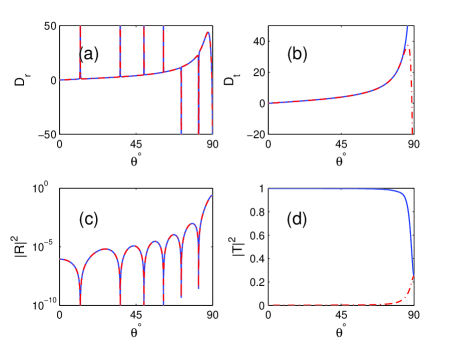
Figure 5: The lateral shift (upper panel) and reflection(transmission) probability (Lower panel) as a function of incident angle for atomic waves in state $\left|1\right\rangle$(solid line) and state $\left|2\right\rangle$(dash-dotted line) through the red-detuned laser beams with equal Rabi frequencies. the Other parameters are: $L=4$, $\gamma=0.1$, $\Omega_{1}=2$, $\Omega_{2}=2$, $k_{0}=0.8$, $k_{L}=0.1$.

Next, we consider another situation when the incident wave is in the superposition state $\left(\left|1\right\rangle+\left|2\right\rangle\right)/\sqrt{2}$ and $\Omega_{1}=\Omega_{2}$. Now the atomic wave in the laser beam only contains $\left|+\right\rangle$ mode, that is to say, the incident wave only ”see” the potential barrier. Based on the previous analyses, the lateral shifts and reflection intensities of the reflected and transmitted waves should be the same. Additionally, the absence of $\left|0\right\rangle$ mode in the transmission implies no quantum interference happening, therefore the transmission intensities of the atomic waves in states $\left|1\right\rangle$ and $\left|2\right\rangle$ should also be equal. Figure 4 verifies these conclusions.

If carefully examining the lateral shifts of transmitted wave in Figs. 2, 3 and 4, one can find that a vanishing transmission intensity is not necessary to observe a large peak of lateral shift. For example, Fig. 3(b) shows a large positive lateral shift of atomic wave in state $\left|2\right\rangle$ near the critical angle, while the corresponding transmission intensity is about $0.6$ [Fig. 3(d)], which is very helpful to experimentally measure such large Goos-Hänchen-like lateral shift of atomic wavepacket.

Finally we study the lateral shifts in the red-detuned case, i.e., $\Delta_{0}=-25$. Different from the blue detuned case, the scattering properties of atomic waves in states $\left|1\right\rangle$ and $\left|2\right\rangle$ are mainly determined by $\left|-\right\rangle$ and $\left|0\right\rangle$ modes, i.e., $\left|1\right\rangle\approx-1/\sqrt{2}\left(\left|-\right\rangle-\left|0\right\rangle\right)$ and $\left|2\right\rangle\approx-1/\sqrt{2}\left(\left|-\right\rangle+\left|0\right\rangle\right)$. Since Re$\left(V_{-}\right)$ is negative for all incident angles, $\left|-\right\rangle$ mode corresponds to a potential well. Lateral shift $D_{r,t}$ and intensity $\left|R\right|^{2}\left(\left|T\right|^{2}\right)$ of reflected and transmitted waves are displayed in Fig. 5 as a function of the incident angle $\theta$. One can see that there are many large positive and negative peaks on the lateral shift curves of reflected waves in states $\left|1\right\rangle$ and $\left|2\right\rangle$, which are caused by the resonance scattering by the potential well. The lateral shift of reflected waves in states $\left|1\right\rangle$ and $\left|2\right\rangle$ are equal, which is similar to the blue detuned case. The reason is that only $\left|-\right\rangle$ mode contributes to the reflected waves. As discussed before, the quantum interference between $\left|-\right\rangle$ and $\left|0\right\rangle$ modes leads to unequal lateral shifts and transmission intensities of transmitted waves in states $\left|1\right\rangle$ and $\left|2\right\rangle$, which is verified by Figs. 5(b) and 5(d).

5 Conclusion

In this work we have investigated the Goos-Hänchen-like lateral shifts of a three-level atomic matter wavepacket obliquely impinging on the ”medium slab” made up of two super-Gaussian laser beams. We have obtained the lateral shifts by expansion of transmission and reflection coefficients. Results show that the lateral shifts can be either positive or negative dependent on the incident angle and atomic states. Different from two-level situation, quantum interference between dressed states manifests itself in the transmission intensity and the corresponding lateral shift of transmitted waves, while it has no influence on the properties of reflected waves.

In particular, we find that there are large lateral shifts with considerable transmission intensities of atomic wave, which is necessary for high sensitive measurements of lateral shifts in experiments.

Additionally, the involving the decay of upper level of the atom will result a loss of atom number, hence the total probability flux is less than one.

Appendix

Here we present the detailed derivation of the transmission and reflection coefficients of the three level atom. Considering an atomic plane wave with incident energy $E=\hbar^{2}k_{0}^{2}/2m$ and initial value $In=\left(In_{1},In_{2},In_{3}\right)^{T}$ incident on the potential. Due to no coupling between different internal states, the scattering solution for Eqs. (8) outside the laser beam is

$$\left(\begin{array}[]{c}\psi_{1}\\ \psi_{2}\\ \psi_{3}\end{array}\right)=\left\{\begin{array}[]{lll}\left(\begin{array}[]{c}In_{1}e^{ik_{1}x}+R_{1}e^{-ik_{1}x}\\ In_{2}e^{ik_{2}x}+R_{2}e^{-ik_{2}x}\\ In_{3}e^{ik_{3}x}+R_{3}e^{-ik_{3}x}\end{array}\right)e^{-iE_{x}t/\hbar}&,&x\leqslant 0\\ \left(\begin{array}[]{c}T_{1}e^{ik_{1}x}\\ T_{2}e^{ik_{2}x}\\ T_{3}e^{ik_{3}x}\end{array}\right)e^{-iE_{x}t/\hbar}&,&x\geqslant L\end{array}\right.$$ (39)

where the wave vectors in free space $k_{1}=k_{2}=k_{0}$ and $k_{3}=\sqrt{k_{1}^{2}+2m\Delta/\hbar}$. $T=\left(T_{1},T_{2},T_{3}\right)^{T}$ and $R=\left(R_{1},R_{2},R_{3}\right)^{T}$, respectively, are the transmission and reflection coefficients of the wave in states $\left|1\right\rangle$, $\left|2\right\rangle$ and $\left|3\right\rangle$. In the laser beam, the lights couple the different atomic internal states $\left|1\right\rangle$ and $\left|2\right\rangle$ to state $\left|3\right\rangle$, described by the coupled equation (8). To diagonalize the coupled equation (8), here we introduce three dressed states

$$\left|\pm\right\rangle=\frac{\left(\Omega_{1}\left|1\right\rangle+\Omega_{2}\left|2\right\rangle+\left(\Delta\mp\tilde{\Delta}\right)\left|3\right\rangle\right)}{\sqrt{\Omega_{1}^{2}+\Omega_{2}^{2}+\left(\Delta\mp\tilde{\Delta}\right)^{2}}}$$ (40)

$$\left|0\right\rangle=\frac{1}{\sqrt{\Omega_{1}^{2}+\Omega_{2}^{2}}}\left(\Omega_{2}\left|1\right\rangle-\Omega_{1}\left|2\right\rangle\right)$$ (41)

When we project the coupled equation (8) onto this dressed state basis, the equation decouples. With this preparation, we finally find the scattering solution in the laser beam taking the form

$$\left(\begin{array}[]{c}\psi_{1}\\ \psi_{2}\\ \psi_{3}\end{array}\right)=U\left(\begin{array}[]{c}A_{+}e^{p_{+}x}+B_{+}e^{-p_{+}x}\\ A_{0}e^{p_{0}x}+B_{0}e^{-p_{0}x}\\ A_{-}e^{p_{-}x}+B_{-}e^{-p_{-}x}\end{array}\right)e^{-iE_{x}t/\hbar}$$ (48)

where $p_{\pm,0}=\sqrt{2mV_{\pm,0}/\hbar^{2}-k_{0}^{2}}$.

With the continuation condition of wave function $\psi$ and its derivative at the boundary of the potential, we obtain following equations

$$\left(\begin{array}[]{c}In_{1}\\ In_{2}\\ In_{3}\end{array}\right)+\left(\begin{array}[]{c}R_{1}\\ R_{2}\\ R_{3}\end{array}\right)=U\left(\begin{array}[]{c}A_{+}+B_{+}\\ A_{0}+B_{0}\\ A_{-}+B_{-}\end{array}\right)$$ (58)

$$i\left(\begin{array}[]{c}k_{1}In_{1}\\ k_{2}In_{2}\\ k_{3}In_{3}\end{array}\right)-i\left(\begin{array}[]{c}k_{1}R_{1}\\ k_{2}R_{2}\\ k_{3}R_{3}\end{array}\right)=U\left(\begin{array}[]{c}p_{+}A_{+}-p_{+}B_{+}\\ p_{0}A_{0}-p_{0}B_{0}\\ p_{-}A_{-}-p_{-}B_{-}\end{array}\right)$$ (68)

$$U\left(\begin{array}[]{c}A_{+}e^{p_{+}L}+B_{+}e^{-p_{+}L}\\ A_{0}e^{p_{0}L}+B_{0}e^{-p_{0}L}\\ A_{-}e^{p_{-}L}+B_{-}e^{-p_{-}L}\end{array}\right)=\left(\begin{array}[]{c}T_{1}e^{ik_{1}L}\\ T_{2}e^{ik_{1}L}\\ T_{3}e^{ik_{3}L}\end{array}\right)$$ (75)

$$U\left(\begin{array}[]{c}p_{+}A_{+}e^{p_{+}L}-p_{+}B_{+}e^{-p_{+}L}\\ p_{0}A_{0}e^{p_{0}L}-p_{0}B_{0}e^{-p_{0}L}\\ p_{-}A_{-}e^{p_{-}L}-p_{-}B_{-}e^{-p_{-}L}\end{array}\right)=\left(\begin{array}[]{c}ik_{1}T_{1}e^{ik_{1}L}\\ ik_{1}T_{2}e^{ik_{1}L}\\ ik_{3}T_{3}e^{ik_{3}L}\end{array}\right)$$ (82)

For mathematical simplification, here we define the matrixes

$$W =\left(\begin{array}[]{ccc}e^{p_{+}L}&0&0\\ 0&e^{p_{0}L}&0\\ 0&0&e^{p_{-}L}\end{array}\right) K =\left(\begin{array}[]{ccc}ik_{1}&0&0\\ 0&ik_{2}&0\\ 0&0&ik_{3}\end{array}\right)$$ (89)

$$E =\left(\begin{array}[]{ccc}e^{ik_{1}L}&0&0\\ 0&e^{ik_{2}L}&0\\ 0&0&e^{ik_{3}L}\end{array}\right) P =\left(\begin{array}[]{ccc}p_{+}&0&0\\ 0&p_{0}&0\\ 0&0&p_{-}\end{array}\right)$$ (96)

Then Eqs. (32)–(35) become matrix equations

$$In+R=U\left(A+B\right)$$ (97)

$$K\left(In-R\right)=UP\left(A-B\right)$$ (98)

$$U\left(WA+W^{-1}B\right)=T$$ (99)

$$UP\left(WA-W^{-1}B\right)=KT$$ (100)

By some simple calculation we obtain the transmission coefficient

$$T=4F^{-1}KIn$$ (101)

with

$$F =\left(KU+UP\right)W^{-1}\left(U^{-1}+P^{-1}U^{-1}K\right)$$

$$+\left(KU-UP\right)W\left(U^{-1}-P^{-1}U^{-1}K\right)$$ (102)

and the reflection coefficient

$$R=-G^{-1}DIn$$ (103)

with

$$G =\left(KU-UP\right)W\left(U^{-1}-P^{-1}U^{-1}K\right)$$

$$+\left(KU+UP\right)W^{-1}\left(U^{-1}+P^{-1}U^{-1}K\right)$$ (104)

and

$$D =\left(KU-UP\right)W\left(U^{-1}+P^{-1}U^{-1}K\right)$$

$$+\left(KU+UP\right)W^{-1}\left(U^{-1}-P^{-1}U^{-1}K\right)$$ (105)

References

- [1] F. Goos and H. Hänchen, “Ein neuer und fundamentaler Versuch zur Totalreflexion,”Ann. Phys. 1, 333 (1947).
- [2] J. Picht, “Beitrag zur Theorie der Totalreflexion,” Ann. Phys.(Leipzig) 3, 433 (1929).
- [3] I. Newton, Optick (Dover, London, 1952).
- [4] K. Artmann, “Calculation of the Lateral Shift of Totally Reflected Beams,”Ann. Phys.(Leipzig) 2, 87 (1948); C.V. Fragstein, “On the Lateral Shift of Totally Reflected Light Beams,” Ann. Phys.(Leipzig) 4, 271 (1949).
- [5] R.H. Renard, “Total Reflection: A New Evaluation of the Goos-Hänchen Shift,” J. Opt. Soc. Am. 54, 1190 (1964).
- [6] Y. Wan, Z. Zheng, W. Kong, Y. Liu, Z. Lu, and Y. Bian, “Direct experimental observation of giant Goos-Hänchen shifts from bandgap-enhanced total internal reflection,” Opt Lett. 36, 3539 (2011).
- [7] I.V. Shadrivov, A.A. Zharov, and Y.S. Kivshar, “ Giant Goos-Hanchen effect at the reflection from left-handed metamaterials,” Appl. Phys. Lett. 83, 2713 (2003).
- [8] O. Emile, T. Galstyan, A. LeFloch, and F. Bretenaker, “Measurement of the Nonlinear Goos-Hänchen Effect for Gaussian Optical Beams,” Phys. Rev. Lett. 75, 1511 (1995).
- [9] C.F. Li, “Negative lateral shift of a light beam transmitted through a dielectric slab and interaction of boundary effects,” Phys. Rev. Lett. 91, 133903 (2003).
- [10] L.G. Wang and S.Y. Zhu, “Giant Lateral shift of a light beam at the defect mode in One-dimensional photonic crystals,” Opt. Lett. 31, 101(2006).
- [11] H.M. Lai and S.W. Chan, “Large and negative Goos–Hänchen shift near the Brewster dip on reflection from weakly absorbing media,” Opt. Lett. 27, 680 (2002).
- [12] Ziauddin and Sajid Qamar, “Gain-assisted control of the Goos-Hänchen shift,” Phys. Rev. A 84, 053844 (2011).
- [13] X.B. Yin and L Hesselink, “Goos-Hänchen shift surface plasmon resonance sensor,” Appl. Phys. Lett. 89, 261108 (2006).
- [14] Bin Zhao and Lei Gao, “Temperature-dependent Goos-Hänchen shift on the interface of metal/dielectric composites,” Optics Express 17, 21433 (2009).
- [15] T Sakata, H Togo, and F Shimokawa, “ Reflection-type 2x2 optical waveguide switch using the Goos-Hdnchen shift effect,” Appl. Phys. Lett. 76, 2841 (2000).
- [16] A. Gedeon, “Observation of the lateral displacement of surface acoustic beams reflected at boundaries of layered substrates,” Appl. Phys. 3, 397 (1974).
- [17] L.W. Zeng and RX Song, “Lateral shift of acoustic wave at interface between double-positive and double-negative media,” Phys. Lett. A 358, 484 (2006).
- [18] V Regnier, “Delayed reflection in a stratified acoustic strip,” Mathematical methods in the applied sciences 28, 185 (2005).
- [19] H. Hora, “Zur seitenversetzung bei der totalreflexion von matteriewellen,” Optik 17, 409 (1960).
- [20] S.C. Miller and N. Ashby, “Shifts of Electron Beam Position Due to Total Reflection at a Barrier,” Phys. Rev. Lett. 29,740 (1972).
- [21] D.M. Fradkin and R.J. Kashuba, “Spatial displacement of electrons due to multiple total reflections,” Phys. Rev. D 9, 2775 (1974).
- [22] M. Mâaza and B. Pardo, “On the possibility to observe the longitudinal Goos-Hänchen shift with cold neutrons,” Optics Communications 142, 84 (1997).
- [23] V.K. Ignatovich, “Neutron reflection from condensed matter, the Goos-Hanchen effect and coherence,” Phys. Lett. A 322, 36 (2004).
- [24] Z. T. Lu, K. L. Corwin, M. J. Renn, M. H. Anderson, E. A. Cornell, and C. E. Wieman, “Low-Velocity Intense Source of Atoms from a Magneto-optical Trap,” Phys. Rev. Lett. 77, 3331 (1996).
- [25] T. M. Roach, H. Abele, M. G. Boshier, H. L. Grossman, K. P. Zetie, and E. A. Hinds, “Realization of a Magnetic Mirror for Cold Atoms,” Phys. Rev. Lett. 75, 629 (1995).
- [26] M. Morinaga, M. Yasuda, T. Kishimoto, F. Shimizu, J. I. Fujita, and S. Matsui, “Holographic Manipulation of a Cold Atomic Beam,” Phys. Rev. Lett. 77, 802 (1996).
- [27] W.P. Zhang and B.C. Sanders, “ Atomic beamsplitter: reflection and transmission by a laser beam,” J. phys. B 27, 795 (1994).
- [28] J. Martina and T. Bastinb, “Transmission of ultracold atoms through a micromaser: detuning effects,” Eur. Phys. J. D 29, 133 (2004).
- [29] J. H. Huang, Z. L. Duan, H. Y. Ling, and W. P. Zhang, “Goos-Hänchen-like shifts in atom optics,” Phys. Rev. A 77, 063608 (2008).
- [30] J.S. Liu and M.R. Taghizadeh, “Iterative algorithm for the design of diffractive phase elements for laser beam shaping,” OPt. Lett. 27, 1463 (2002).
- [31] P.A. Bélanger, R.L. Lachance, and C. Paré, “Super-Gaussian output from a CO2 laser by using a graded-phase mirror resonator,” Opt. Lett. 17, 739 (1992).
- [32] G.J. Dong, S. Edvadsson, W. Lu, and P.F. Barker, “Super-Gaussian mirror for high-field-seeking molecules,” Phys. Rev. A 72, 031605(R) (2005).
- [33] C.W. Hsue and T. Tamir, “Lateral displacement and distortion of beams incident upon a transmitting-layer configuration,” J. Opt. Soc. Am. A 2, 978 (1985).
- [34] Z.L. Duan and W.P. Zhang, “Failures of the adiabatic approximation in quantum tunneling time,” Phys. Rev. A 86, 064101 (2012).