Constraint Reduction using Marginal Polytope Diagrams for MAP LP Relaxations

Abstract

LP relaxation-based message passing algorithms provide an effective tool for MAP inference over Probabilistic Graphical Models. However, different LP relaxations often have different objective functions and variables of differing dimensions, which presents a barrier to effective comparison and analysis. In addition, the computational complexity of LP relaxation-based methods grows quickly with the number of constraints. Reducing the number of constraints without sacrificing the quality of the solutions is thus desirable.

We propose a unified formulation under which existing MAP LP relaxations may be compared and analysed. Furthermore, we propose a new tool called Marginal Polytope Diagrams. Some properties of Marginal Polytope Diagrams are exploited such as node redundancy and edge equivalence. We show that using Marginal Polytope Diagrams allows the number of constraints to be reduced without loosening the LP relaxations. Then, using Marginal Polytope Diagrams and constraint reduction, we develop three novel message passing algorithms, and demonstrate that two of these show a significant improvement in speed over state-of-art algorithms while delivering a competitive, and sometimes higher, quality of solution.

1 Introduction

Linear Programming (LP) relaxations have been used to approximate the maximum a posteriori (MAP) inference of Probabilistic Graphical Models (PGMs) Koller and Friedman (2009) by enforcing local consistency over edges or clusters. An attractive property of this approach is that it is guaranteed to find the optimal MAP solution when the labels are integers. This is particularly significant in light of the fact that Kumar et al.showed that LP relaxation provides a better approximation than Quadratic Programming relaxation and Second Order Cone Programming relaxation Kumar et al (2009). Despite their success, there remain a variety of large-scale problems that off-the-shelf LP solvers can not solve Yanover et al (2006). Moreover, it has been shown Yanover et al (2006); Sontag et al (2008) that LP relaxations have a large gap between the dual objective and the decoded primal objective and fail to find the optimal MAP solution in many real-world problems.

In response to this shortcoming a number of dual message passing methods have been proposed including Dual Decompositions Komodakis et al (2007); Sontag et al (2011, 2012) and Generalised Max Product Linear Programming (GMPLP) Globerson and Jaakkola (2007). These methods can still be computationally expensive when there are a large number of constraints in the LP relaxations. It is desirable to reduce the number of constraints in order to reduce computational complexity without sacrificing the quality of the solution. However, this is non-trivial, because for a MAP inference problem the dimension of the primal variable can be different in various LP relaxations. This also presents a barrier for effectively comparing the quality of two LP relaxations and their corresponding message passing methods. Furthermore, these message-passing methods may get stuck in non-optimal solutions due to the non-smooth dual objectives Schwing et al (2012); Hazan and Shashua (2010); Meshi et al (2012).

Our contributions are: 1) we propose a unified form for MAP LP relaxations, under which existing MAP LP relaxations can be rewritten as constrained optimisation problems with variables of the same dimension and objective; 2) we present a new tool which we call the Marginal Polytope Diagram to effectively compare different MAP LP relaxations. We show that any MAP LP relaxation in the above unified form has a Marginal Polytope Diagram, and vice versa. We establish propositions to conveniently show the equivalence of seemingly different Marginal Polytope Diagrams; 3) Using Marginal Polytope Diagrams, we show how to safely reduce the number of constraints (and consequently the number of messages) without sacrificing the quality of the solution, and propose three new message passing algorithms in the dual; 4) we show how to perform message passing in the dual without computing and storing messages (via updating the beliefs only and directly); 5) we propose a new cluster pursuit strategy.

2 MAP Inference and LP Relaxations

We consider MAP inference over factor graphs with discrete states. For generality, we will use higher order potentials (where possible) throughout the paper.

2.1 MAP inference

Assume that there are $n$ variables $X_{1},\cdots,X_{n}$, each taking discrete states $x_{i}\in$ Vals$(X_{i})$. Let $\operatorname{\mathcal{V}}=\{1,\cdots,n\}$ denote the node set, and let $\operatorname{\mathcal{C}}$ be a collection of subsets of $\operatorname{\mathcal{V}}$. $\operatorname{\mathcal{C}}$ has an associated group of potentials $\boldsymbol{\theta}=\{\theta_{c}(\operatorname{\mathbf{x}}_{c})\in\mathbb{R}|c\in\operatorname{\mathcal{C}}\}$, where $\operatorname{\mathbf{x}}_{c}=[x_{i}]_{i\in c}$. Given a graph $G=(\operatorname{\mathcal{V}},\operatorname{\mathcal{C}})$ and potentials $\boldsymbol{\theta}$, we consider the following exponential family distribution (Wainwright and Jordan, 2008):

$$p(\operatorname{\mathbf{x}}|\boldsymbol{\theta})=\frac{1}{Z}\exp\left(\sum_{c\in\operatorname{\mathcal{C}}}\theta_{c}(\operatorname{\mathbf{x}}_{c})\right),$$ (1)

where $\operatorname{\mathbf{x}}=[x_{1},x_{2},\ldots,x_{n}]\in\operatorname{\mathcal{X}}$, and $Z=\sum_{\operatorname{\mathbf{x}}\in\operatorname{\mathcal{X}}}\exp(\sum_{c\in\operatorname{\mathcal{C}}}\theta_{c}(\operatorname{\mathbf{x}}_{c}))$ is known as a normaliser, or partition function. The goal of MAP inference is to find the MAP assignment, $\operatorname{\mathbf{x}}^{*}$, that maximises $p(\operatorname{\mathbf{x}}|\boldsymbol{\theta})$. That is

$$\operatorname{\mathbf{x}}^{*}=\mathop{\mathrm{argmax}}_{\operatorname{\mathbf{x}}}\sum_{c\in\mathcal{C}}\theta_{c}(\operatorname{\mathbf{x}}_{c}).$$ (2)

Here we slightly generalise the notation of $\operatorname{\mathbf{x}}_{c}$ to $\operatorname{\mathbf{x}}_{s}=[x_{i}]_{i\in s}$, $\operatorname{\mathbf{x}}_{t}=[x_{i}]_{i\in t}$ and $\operatorname{\mathbf{x}}_{f}=[x_{i}]_{i\in f}$ where $s,t,f$ are subsets of $\operatorname{\mathcal{V}}$ reserved for later use.

2.2 Linear Programming Relaxations

By introducing

$$\operatorname{\boldsymbol{\mu}}=(\mu_{c}(\operatorname{\mathbf{x}}_{c}))_{c\in\operatorname{\mathcal{C}}},$$ (3)

the MAP inference problem can be written as an equivalent Linear Programming (LP) problem as follows

$$\displaystyle{\operatorname{\boldsymbol{\mu}}^{*}=\mathop{\mathrm{argmax}}_{\operatorname{\boldsymbol{\mu}}\in\operatorname{\mathcal{M}}(G)}\sum_{c\in\operatorname{\mathcal{C}}}\sum_{\operatorname{\mathbf{x}}_{c}}\mu_{c}(\operatorname{\mathbf{x}}_{c})\theta_{c}(\operatorname{\mathbf{x}}_{c})},$$ (4)

in which the feasible set, $\operatorname{\mathcal{M}}(G)$, is known as the marginal polytope (Wainwright and Jordan, 2008), defined as follows

$$\left\{\operatorname{\boldsymbol{\mu}}\left|\begin{array}[]{l}q(\operatorname{\mathbf{x}})\geqslant 0,~{}\forall\operatorname{\mathbf{x}}\\ \sum_{\operatorname{\mathbf{x}}}q(\operatorname{\mathbf{x}})=1\\ \sum_{\operatorname{\mathbf{x}}_{\operatorname{\mathcal{V}}\setminus c}}q(\operatorname{\mathbf{x}})=\mu_{c}(\operatorname{\mathbf{x}}_{c}),\forall c\in\operatorname{\mathcal{C}},\operatorname{\mathbf{x}}_{c}\\ \end{array}\right.\right\}.$$ (8)

Here the first two groups of constraints specify that $q(\operatorname{\mathbf{x}})$ is a distribution over $\operatorname{\mathcal{X}}$, and we refer to the last group of constraints as the global marginalisation constraint, which guarantees that for arbitrary $\operatorname{\boldsymbol{\mu}}$ in $\operatorname{\mathcal{M}}(G)$, all $\mu_{c}(\operatorname{\mathbf{x}}_{c}),c\in\operatorname{\mathcal{C}}$ can be obtained by marginalisation from a common distribution $q(\operatorname{\mathbf{x}})$ over $\operatorname{\mathcal{X}}$. In general, exponentially many inequality constraints (i.e. $q(\operatorname{\mathbf{x}})\geqslant 0,~{}\forall\operatorname{\mathbf{x}}$) are required to define a marginal polytope, which makes the LP hard to solve. Thus (4) is often relaxed with a local marginal polytope $\operatorname{\mathcal{M}}_{L}(G)$ to obtain the following LP relaxation

$$\displaystyle{\operatorname{\boldsymbol{\mu}}^{*}=\mathop{\mathrm{argmax}}_{\operatorname{\boldsymbol{\mu}}\in\operatorname{\mathcal{M}}_{L}(G)}\sum_{c\in\operatorname{\mathcal{C}}}\sum_{\operatorname{\mathbf{x}}_{c}}\mu_{c}(\operatorname{\mathbf{x}}_{c})\theta_{c}(\operatorname{\mathbf{x}}_{c})}.$$ (9)

Different LP relaxation schemes define different local marginal polytopes. A typical local marginal polytope defined in Sontag et al (2011); Hazan and Shashua (2010) is as follows:

$$\left\{\operatorname{\boldsymbol{\mu}}\left|\begin{array}[]{l}\sum\limits_{\operatorname{\mathbf{x}}_{c\setminus\{i\}}}\mu_{c}(\operatorname{\mathbf{x}}_{c})=\mu_{i}(x_{i}),\forall c\in\operatorname{\mathcal{C}},i\in c,x_{i}\\ \mu_{c}(\operatorname{\mathbf{x}}_{c})\geqslant 0,\sum\limits_{\operatorname{\mathbf{x}}_{c}}\mu_{c}(\operatorname{\mathbf{x}}_{c})=1,\forall c\in\operatorname{\mathcal{C}},\operatorname{\mathbf{x}}_{c}\end{array}\right.\right\}.$$ (12)

Compared to the marginal polytope, for arbitrary $\operatorname{\boldsymbol{\mu}}$ in a local marginal polytope, all $\operatorname{\boldsymbol{\mu}}_{c}(\operatorname{\mathbf{x}}_{c})$ may not be the marginal distributions of a common distribution $q(\operatorname{\mathbf{x}})$ over $\operatorname{\mathcal{X}}$, but there are much fewer constraints in local marginal polytope. As a result, the LP relaxation can be solved more efficiently. This is of particular practical significance because state-of-the-art interior point or simplex LP solvers can only handle problems with up to a few hundred thousand variables and constraints while many real-world datasets demand far more variables and constraints (Yanover et al, 2006; Kumar et al, 2009).

Several message passing-based approximate algorithms (Globerson and Jaakkola, 2007; Sontag et al, 2008, 2012) have been proposed to solve large scale LP relaxations. Each of them applies coordinate descent to the dual objective of an LP relaxation problem with a particular local marginal polytope. Different local marginal polytopes use different local marginalisation constraints, which leads to different dual problems and hence different message updating schemes.

2.3 Generalised Max Product Linear Programming

Globerson and Jaakkola (2007) showed that LP relaxations can also be solved by message passing, known as Max Product LP (MPLP) when only node and edge potentials are considered, or Generalised MPLP (GMPLP) (see Section 6 of (Globerson and Jaakkola, 2007)) when potentials over clusters are considered.

In GMPLP, they define $\operatorname{\mathcal{I}}=\{s|s=c\cap c^{\prime};c,c^{\prime}\in\operatorname{\mathcal{C}}\}$, and

$$\operatorname{\boldsymbol{\mu}}^{g}=(\mu_{c}(\operatorname{\mathbf{x}}_{c}),\mu_{s}(\operatorname{\mathbf{x}}_{s}))_{c\in\operatorname{\mathcal{C}},s\in\operatorname{\mathcal{I}}}.$$ (13)

Then they consider the following LP relaxation

$$\displaystyle{\operatorname{\boldsymbol{\mu}}^{g*}=\mathop{\mathrm{argmax}}_{\operatorname{\boldsymbol{\mu}}^{g}\in\operatorname{\mathcal{M}}_{L}^{g}(G)}\sum_{c\in\operatorname{\mathcal{C}}}\sum_{\operatorname{\mathbf{x}}_{c}}\mu_{c}(\operatorname{\mathbf{x}}_{c})\theta_{c}(\operatorname{\mathbf{x}}_{c})},$$ (14)

where the local marginal polytope $\operatorname{\mathcal{M}}_{L}^{g}(G)$ is defined as

$$\left\{\boldsymbol{\mu}^{g}\left|\begin{array}[]{l}\mu_{c}(\operatorname{\mathbf{x}}_{c})\geqslant 0,\forall c\in\operatorname{\mathcal{C}},\operatorname{\mathbf{x}}_{c}\\ {\sum\limits_{\operatorname{\mathbf{x}}_{c}}\mu_{c}(\operatorname{\mathbf{x}}_{c})=1,~{}\forall c\in\operatorname{\mathcal{C}}}\\ {\sum\limits_{\operatorname{\mathbf{x}}_{c\setminus s}}\mu_{c}(\operatorname{\mathbf{x}}_{c})=\mu_{s}(\operatorname{\mathbf{x}}_{s}),\forall c\in\mathcal{C},s\in\mathcal{S}_{g}(c),\operatorname{\mathbf{x}}_{s}}\\ \end{array}\right.\right\}$$ (15)

with $\operatorname{\mathcal{S}}_{g}(c)=\{s|s\in\operatorname{\mathcal{I}},s\subseteq c\}$. To derive a desirable dual formulation, they replace the third group of constraints with the following equivalent constraints

$$\mu_{c\setminus s,s}(\operatorname{\mathbf{x}}_{c\setminus s},\operatorname{\mathbf{x}}_{s})=\mu_{c}(\operatorname{\mathbf{x}}_{c}),\quad\forall c\in\mathcal{C},s\in\mathcal{S}_{g}(c),\operatorname{\mathbf{x}}_{c},$$

$$\sum_{\operatorname{\mathbf{x}}_{c\setminus s}}\mu_{c\setminus s,s}(\operatorname{\mathbf{x}}_{c\setminus s},\operatorname{\mathbf{x}}_{s})=\mu_{s}(\operatorname{\mathbf{x}}_{s}),\quad\forall c\in\mathcal{C},s\in\mathcal{S}_{g}(c),\operatorname{\mathbf{x}}_{s}$$

where $\mu_{c\setminus s,s}(\operatorname{\mathbf{x}}_{c\setminus s},\operatorname{\mathbf{x}}_{s})$ is known as the copy variable. Let $\beta_{c\setminus s,s}(\operatorname{\mathbf{x}}_{c\setminus s},\operatorname{\mathbf{x}}_{s})$ be the dual variable associated with the first group of the new constraints above, using standard Lagrangian yields the following dual problem:

$$\min_{\beta} \sum_{s\in\operatorname{\mathcal{I}}}\mathop{\mathrm{max}}_{\operatorname{\mathbf{x}}_{s}}\sum_{c\in\operatorname{\mathcal{C}},s\in\operatorname{\mathcal{S}}_{g}(c)}\mathop{\mathrm{max}}_{\operatorname{\mathbf{x}}_{c\setminus s}}\beta_{c\setminus s,s}(\operatorname{\mathbf{x}}_{c\setminus s},\operatorname{\mathbf{x}}_{s})$$

$$\mathrm{s.t.} ~{}\theta_{c}(\operatorname{\mathbf{x}}_{c})=\sum_{s\in\mathcal{S}_{g}(c)}\beta_{c\setminus s,s}(\operatorname{\mathbf{x}}_{c\setminus s},\operatorname{\mathbf{x}}_{s}),~{}\forall c\in\operatorname{\mathcal{C}},\operatorname{\mathbf{x}}_{c}.$$ (16)

Let $\lambda_{c\rightarrow s}(\operatorname{\mathbf{x}}_{s})=\mathop{\mathrm{max}}_{\operatorname{\mathbf{x}}_{c\setminus s}}\beta_{c\setminus s,s}(\operatorname{\mathbf{x}}_{c\setminus s},\operatorname{\mathbf{x}}_{s})$, they use a coordinate descent method to minimise the dual by picking up a particular $c\in\operatorname{\mathcal{C}}$ and updating all $\lambda^{*}_{c\rightarrow s}(\operatorname{\mathbf{x}}_{s})$ as following:

$$\lambda^{*}_{c\rightarrow s}(\operatorname{\mathbf{x}}_{s})=-\lambda_{s}^{-c}(\operatorname{\mathbf{x}}_{s})+$$

$$\frac{1}{\left|\mathcal{S}_{g}(c)\right|}\mathop{\mathrm{max}}\limits_{\operatorname{\mathbf{x}}_{c\setminus s}}\bigg{[}\theta_{c}(\operatorname{\mathbf{x}}_{c})+\sum\limits_{\hat{s}\in\mathcal{S}_{g}(c)}\lambda_{\hat{s}}^{-c}(\operatorname{\mathbf{x}}_{\hat{s}})\bigg{]},\forall s\in\operatorname{\mathcal{S}}_{g}(c),\operatorname{\mathbf{x}}_{s}$$ (17)

where $\lambda_{s}^{-c}(\operatorname{\mathbf{x}}_{s})=\sum_{\hat{c}\in\{\bar{c}|\bar{c}\in\operatorname{\mathcal{C}},\bar{c}\neq c,s\in\operatorname{\mathcal{S}}_{g}(\bar{c})\}}\lambda_{\hat{c}\rightarrow s}(\operatorname{\mathbf{x}}_{s})$. At each iteration the dual objective always decreases, thus guaranteeing convergence. Under certain conditions GMPLP finds the exact solution. Sontag et al.(Sontag et al, 2008) extended this idea by iteratively adding clusters and reported faster convergence empirically.

2.4 Dual Decomposition

Dual Decomposition (Komodakis et al, 2007; Sontag et al, 2011) explicitly splits node potentials (those potentials of order 1) from cluster potentials with order greater than 1, and rewrites the MAP objective (2) as

$$\sum_{i\in\operatorname{\mathcal{V}}}\theta_{i}(x_{i})+\sum_{f\in\mathcal{F}}\theta_{f}(\operatorname{\mathbf{x}}_{f}),$$ (18)

where $\mathcal{F}=\{f|f\in\operatorname{\mathcal{C}},|f|>1\}$. By defining $\boldsymbol{\mu}^{d}=(\mu_{i}(x_{i}),\mu_{f}(\operatorname{\mathbf{x}}_{f}))_{i\in\operatorname{\mathcal{V}},f\in\operatorname{\mathcal{F}}}$, they consider the following LP relaxation:

$$\max_{\boldsymbol{\mu}^{d}\in\mathcal{M}_{L}^{d}(G)} f_{d}(\operatorname{\boldsymbol{\mu}}^{d})$$

$$f_{d}(\operatorname{\boldsymbol{\mu}}^{d})= \sum_{i\in\operatorname{\mathcal{V}}}\sum_{x_{i}}\mu_{i}(x_{i})\theta_{i}(x_{i})+\sum_{f\in\mathcal{F}}\sum_{\operatorname{\mathbf{x}}_{f}}\mu_{f}(\operatorname{\mathbf{x}}_{f})\theta_{f}(\operatorname{\mathbf{x}}_{f})$$ (19)

with a different local marginal polytope $\operatorname{\mathcal{M}}_{L}^{d}(G)$ defined as

$$\left\{\boldsymbol{\mu}^{d}\geqslant 0\left|\begin{matrix}\sum_{x_{i}}\mu_{i}(x_{i})=1,\forall i\in\operatorname{\mathcal{V}}\\ \sum_{\operatorname{\mathbf{x}}_{f/\{i\}}}\mu_{f}(\operatorname{\mathbf{x}}_{f})=\mu_{i}(x_{i}),\forall f\in\mathcal{F},i\in f,x_{i}\\ \end{matrix}\right.\right\}.$$ (20)

Let $\lambda_{fi}(x_{i})$ be the Lagrangian multipliers corresponding to each $\sum_{\operatorname{\mathbf{x}}_{f\setminus\{i\}}}\mu_{f}(\operatorname{\mathbf{x}}_{f})=\mu_{i}(x_{i})$ for each $f\in\operatorname{\mathcal{F}},i\in f,x_{i}$, one can show that the standard Lagrangian duality is

$$L(\lambda) =\sum_{i\in\operatorname{\mathcal{V}}}\max_{x_{i}}\Big{(}\theta_{i}(x_{i})+\sum_{f\in\{f^{\prime}|f^{\prime}\in\operatorname{\mathcal{F}},i\in f^{\prime}\}}\lambda_{fi}(x_{i})\Big{)}$$

$$+\sum_{f\in\mathcal{F}}\max_{\operatorname{\mathbf{x}}_{f}}\Big{(}\theta_{f}(\operatorname{\mathbf{x}}_{f})-\sum_{i\in f}\lambda_{fi}(x_{i})\Big{)}.$$ (21)

Subgradient or coordinate descent can be used to minimise the dual objective. Since the Dual Decomposition using coordinate descent is closely related to GMPLP and the unified form which we will present, we give the update rule derived by coordinate descent below,

$$\lambda^{*}_{fi}(x_{i})=-\theta_{i}(x_{i})-\lambda_{i}^{-f}(x_{i})+$$

$$\frac{1}{|f|}\max_{\operatorname{\mathbf{x}}_{f\setminus\{i\}}}\Big{[}\theta_{f}(\operatorname{\mathbf{x}}_{f})+\sum_{\hat{i}\in f}\theta_{\hat{i}}(x_{\hat{i}})+\sum_{\hat{i}\in f}\lambda_{\hat{i}}^{-f}(x_{\hat{i}})\Big{]},\forall i\in f,x_{i}$$ (22)

where $f$ is a particular cluster from $\operatorname{\mathcal{F}}$, and $\lambda_{i}^{-f}(x_{i})=\sum_{\hat{f}\in\{\bar{f}|\bar{f}\in\operatorname{\mathcal{F}},\bar{f}\neq f,i\in\bar{f}\}}\lambda_{\hat{f}i}(x_{i})$.

Compared to GMPLP, the local marginal polytope in the Dual Decomposition has much fewer constraints. In general for an arbitrary graph $G=(\operatorname{\mathcal{V}},\operatorname{\mathcal{C}})$, $\operatorname{\mathcal{M}}_{L}^{d}(G)$ is looser than $\operatorname{\mathcal{M}}_{L}^{g}(G)$ (i.e. $\operatorname{\mathcal{M}}_{L}^{d}(G)\supseteq\operatorname{\mathcal{M}}_{L}^{g}(G)$) .

2.5 Dual Decomposition with cycle inequalities

Recently, Sontag et al.Sontag et al (2012) proposed a Dual Decomposition with cycle inequalities considering the following LP relaxation

$$\operatorname{\boldsymbol{\mu}}^{d*}=\max_{\mu\in\operatorname{\mathcal{M}}^{o}_{L}(G)}f_{d}(\operatorname{\boldsymbol{\mu}}^{d})$$ (23)

with a local marginal polytope $\operatorname{\mathcal{M}}^{o}_{L}(G)$,

$$\left\{\boldsymbol{\mu}^{d}\left|\begin{matrix}\sum_{x_{i}}\mu_{i}(x_{i})=1,\forall i\in\operatorname{\mathcal{V}},x_{i}\\ \sum\limits_{\operatorname{\mathbf{x}}_{f/\{i\}}}\mu_{f}(\operatorname{\mathbf{x}}_{f})=\mu_{i}(x_{i}),\forall f\in\operatorname{\mathcal{F}},i\in f,x_{i}\\ \sum\limits_{\operatorname{\mathbf{x}}_{f/e}}\mu_{f}(\operatorname{\mathbf{x}}_{f})=\mu_{e}(\operatorname{\mathbf{x}}_{e}),\forall f,e\in\operatorname{\mathcal{F}},e\subset f,\operatorname{\mathbf{x}}_{e},|e|=2,|f|\geq 3\\ \boldsymbol{\mu}^{d}\geqslant 0\end{matrix}\right.\right\}$$

They added cycle inequalities to tighten the problem. Reducing the primal feasible set may reduce the maximum primal objective, which reduces the minimum dual objective. They showed that finding the “tightest” cycles, which maximise the decrease in the dual objective, is NP-hard. Thus, instead, they looked for the most “frustrated” cycles, which correspond to the cycles with the smallest LHS of their cycle inequalities. Searching for “frustrated” cycles, adding the cycles’ inequalities and updating the dual is repeated until the algorithm converges.

3 A Unified View of MAP LP Relaxations

In different LP relaxations, not only the formulations of the objective, but also the dimension of primal variable may vary, which makes comparison difficult. By way of illustration, note that the primal variable in GMPLP is $\operatorname{\boldsymbol{\mu}}^{g}=(\mu_{c}(\operatorname{\mathbf{x}}_{c}),\mu_{s}(\operatorname{\mathbf{x}}_{s}))_{c\in\operatorname{\mathcal{C}},s\in\operatorname{\mathcal{I}}}$, while in Dual Decomposition the primal variable is $\operatorname{\boldsymbol{\mu}}^{d}=\{\mu_{i}(x_{i}),\mu_{f}(\operatorname{\mathbf{x}}_{f})\}_{i\in\operatorname{\mathcal{V}},f\in\operatorname{\mathcal{F}}}$. Although $\operatorname{\boldsymbol{\mu}}^{d}$ can be reformulated to $(\mu_{c}(\operatorname{\mathbf{x}}_{c}))_{c\in\operatorname{\mathcal{C}}}$ if $\operatorname{\mathcal{C}}=\{\{i\}|i\in\operatorname{\mathcal{V}}\}\cup\operatorname{\mathcal{F}}$, the variables $\{\mu_{s}(\operatorname{\mathbf{x}}_{s})\}_{s\in\operatorname{\mathcal{I}}}$ (corresponding to intersections) in GMPLP still do not appear in Dual Decomposition. This shows that the dimensions of the primal variables in GMPLP and Dual Decomposition are different.

3.1 A Unified Formulation

When using the local marginal polytope the objective of the LP relaxation depends only on those $\mu_{c}(\operatorname{\mathbf{x}}_{c}),c\in\operatorname{\mathcal{C}}$. We thus reformulate the LP Relaxation into a unified formulation as follows:

$$\displaystyle{\operatorname{\boldsymbol{\mu}}^{*}=\mathop{\mathrm{argmax}}_{\operatorname{\boldsymbol{\mu}}\in\operatorname{\mathcal{M}}_{L}(G,\operatorname{\mathcal{C}}^{\prime},\operatorname{\mathcal{S}}(\operatorname{\mathcal{C}}^{\prime}))}\sum_{c\in\operatorname{\mathcal{C}}}\sum_{\operatorname{\mathbf{x}}_{c}}\mu_{c}(\operatorname{\mathbf{x}}_{c})\theta_{c}(\operatorname{\mathbf{x}}_{c})},$$ (24)

where $\operatorname{\boldsymbol{\mu}}$ is defined in (3). The local marginal polytope, $\operatorname{\mathcal{M}}_{L}(G,\operatorname{\mathcal{C}}^{\prime},\operatorname{\mathcal{S}}(\operatorname{\mathcal{C}}^{\prime}))$, can be defined in a unified formulation as

$$\left\{\operatorname{\boldsymbol{\mu}}\left|\begin{array}[]{l}\mu_{c}(\operatorname{\mathbf{x}}_{c})\geqslant 0,\forall c\in\operatorname{\mathcal{C}}^{\prime},\operatorname{\mathbf{x}}_{c}\\ \sum\limits_{\operatorname{\mathbf{x}}_{c}}\mu_{c}(\operatorname{\mathbf{x}}_{c})=1,\forall c\in\operatorname{\mathcal{C}}^{\prime}\\ \sum\limits_{\operatorname{\mathbf{x}}_{c\setminus s}}\mu_{c}(\operatorname{\mathbf{x}}_{c})=\mu_{s}(\operatorname{\mathbf{x}}_{s}),\forall c\in\operatorname{\mathcal{C}}^{\prime},s\in\operatorname{\mathcal{S}}(c),\operatorname{\mathbf{x}}_{s}\end{array}\right.\right\}.$$ (28)

Here $\operatorname{\mathcal{C}}^{\prime}$ is what we call an extended cluster set, where each $c\in\operatorname{\mathcal{C}}^{\prime}$ is called an extended cluster. $\operatorname{\mathcal{S}}(\operatorname{\mathcal{C}}^{\prime})=(\operatorname{\mathcal{S}}(c))_{c\in\operatorname{\mathcal{C}}^{\prime}}$, where each $s\in\operatorname{\mathcal{S}}(c)$ is a subset of $c$, which we refer to as a sub-cluster. The choices of $\operatorname{\mathcal{C}}^{\prime}$ and $\operatorname{\mathcal{S}}(\operatorname{\mathcal{C}}^{\prime})$ correspond to existing or even new inference algorithms, which will be shown later, and when specifying $\operatorname{\mathcal{C}}^{\prime}$ and $\operatorname{\mathcal{S}}(\operatorname{\mathcal{C}}^{\prime})$, we require $\operatorname{\mathcal{C}}^{\prime}\cup(\mathop{\cup}_{c\in\operatorname{\mathcal{C}}^{\prime}}\operatorname{\mathcal{S}}(c))\supseteq\operatorname{\mathcal{C}}$.

The first two groups of constraints in $\operatorname{\mathcal{M}}_{L}(G,\operatorname{\mathcal{C}}^{\prime},\operatorname{\mathcal{S}}(\operatorname{\mathcal{C}}^{\prime}))$ ensure that $\forall c\in\operatorname{\mathcal{C}}^{\prime}$, $\mu_{c}(\operatorname{\mathbf{x}}_{c})$ is a distribution over Vals($\operatorname{\mathbf{x}}_{c}$). We refer to the third group of constraints as local marginalisation constraints.

Remarks

The LP formulation in (1) and (2) of (Werner, 2010) may look similar to ours. However, the work of (Werner, 2010) is in fact a special case of ours. In their work, an additional restriction $s\subset c$ for (28) must be satisfied (see (4) in (Werner, 2010)). As a result, their work does not cover the LP relaxations in Sontag et al (2008) and GMPLP, where redundant constraints like $\mu_{c}(\operatorname{\mathbf{x}}_{c})=\mu_{c}(\operatorname{\mathbf{x}}_{c})$ are used to derive a message from one cluster to itself (see Figure 1 of Sontag et al (2008)). Our approach, however, is in fact a generalisation of Sontag et al (2008), GMPLP and Werner (2010).

3.2 Reformulating GMPLP and Dual Decomposition

Here we show that both GMPLP and Dual Decomposition can be reformulated by (24).

Let us start with GMPLP first. Let $\operatorname{\mathcal{C}}^{\prime}$ be $\operatorname{\mathcal{C}}$ and $\operatorname{\mathcal{S}}(\operatorname{\mathcal{C}}^{\prime})$ be $\operatorname{\mathcal{S}}_{g}(\operatorname{\mathcal{C}})=(\operatorname{\mathcal{S}}_{g}(c))_{c\in\operatorname{\mathcal{C}}}$. GMPLP (14) can be reformulated as follows

$$\displaystyle{\operatorname{\boldsymbol{\mu}}^{*}=\mathop{\mathrm{argmax}}_{\operatorname{\boldsymbol{\mu}}\in\operatorname{\mathcal{M}}_{L}(G,\operatorname{\mathcal{C}},\operatorname{\mathcal{S}}_{g}(\operatorname{\mathcal{C}}))}\sum_{c\in\operatorname{\mathcal{C}}}\sum_{\operatorname{\mathbf{x}}_{c}}\mu_{c}(\operatorname{\mathbf{x}}_{c})\theta_{c}(\operatorname{\mathbf{x}}_{c})},$$ (29)

where $\operatorname{\mathcal{M}}_{L}(G,\operatorname{\mathcal{C}},\operatorname{\mathcal{S}}_{g}(\operatorname{\mathcal{C}}))$ is defined as

$$\left\{\operatorname{\boldsymbol{\mu}}\left|\begin{array}[]{l}\mu_{c}(\operatorname{\mathbf{x}}_{c})\geqslant 0,\forall c\in\operatorname{\mathcal{C}},\operatorname{\mathbf{x}}_{c}\\ \sum\limits_{\operatorname{\mathbf{x}}_{c}}\mu_{c}(\operatorname{\mathbf{x}}_{c})=1,\forall c\in\operatorname{\mathcal{C}}\\ \sum\limits_{\operatorname{\mathbf{x}}_{c\setminus s}}\mu_{c}(\operatorname{\mathbf{x}}_{c})=\mu_{s}(\operatorname{\mathbf{x}}_{s}),\forall c\in\operatorname{\mathcal{C}},s\in\operatorname{\mathcal{S}}_{g}(c),\operatorname{\mathbf{x}}_{s}\end{array}\right.\right\}.$$ (33)

We can see that (33) and (15) only differ in the dimensions of their variables $\operatorname{\boldsymbol{\mu}}$ and $\operatorname{\boldsymbol{\mu}}^{g}$ (see (3) and (13)). Since the objectives in (29) and (14) do not depend on $\mu_{s}(\operatorname{\mathbf{x}}_{s}),s\in\operatorname{\mathcal{I}}$ directly, the solutions of the two optimisation problems (29) and (14) are the same on $\operatorname{\boldsymbol{\mu}}$.

For Dual Decomposition, we let $\operatorname{\mathcal{C}}_{d}=\{\{i\}|i\in\operatorname{\mathcal{V}}\}\cup\operatorname{\mathcal{F}}$, and

$$\operatorname{\mathcal{S}}_{d}(c)=\left\{\begin{array}[]{ll}\emptyset,&~{}|c|=1\\ \{\{i\}|i\in\operatorname{\mathcal{C}}\}&~{}|c|>1\end{array}\right..$$ (36)

Let $\operatorname{\mathcal{C}}^{\prime}$ be $\operatorname{\mathcal{C}}_{d}$ and $\operatorname{\mathcal{S}}(\operatorname{\mathcal{C}}^{\prime})$ be $\operatorname{\mathcal{S}}_{d}(\operatorname{\mathcal{C}}_{d})=(\operatorname{\mathcal{S}}_{d}(c))_{c\in\operatorname{\mathcal{C}}_{d}}$. Dual Decomposition (19) can be reformulated as

$$\displaystyle{\operatorname{\boldsymbol{\mu}}^{*}=\mathop{\mathrm{argmax}}_{\operatorname{\boldsymbol{\mu}}\in\operatorname{\mathcal{M}}_{L}(G,\operatorname{\mathcal{C}}_{d},\operatorname{\mathcal{S}}_{d}(\operatorname{\mathcal{C}}_{d}))}\sum_{c\in\operatorname{\mathcal{C}}}\sum_{\operatorname{\mathbf{x}}_{c}}\mu_{c}(\operatorname{\mathbf{x}}_{c})\theta_{c}(\operatorname{\mathbf{x}}_{c})},$$ (37)

where $\operatorname{\mathcal{M}}_{L}(G,\operatorname{\mathcal{C}}_{d},\operatorname{\mathcal{S}}_{d}(\operatorname{\mathcal{C}}_{d}))$ is defined as

$$\left\{\operatorname{\boldsymbol{\mu}}\left|\begin{array}[]{l}\mu_{c}(\operatorname{\mathbf{x}}_{c})\geqslant 0,~{}\forall c\in\operatorname{\mathcal{C}}_{d},\operatorname{\mathbf{x}}_{c}\\ \sum\limits_{\operatorname{\mathbf{x}}_{c}}\mu_{c}(\operatorname{\mathbf{x}}_{c})=1,~{}\forall c\in\operatorname{\mathcal{C}}_{d}\\ \sum\limits_{\operatorname{\mathbf{x}}_{c\setminus s}}\mu_{c}(\operatorname{\mathbf{x}}_{c})=\mu_{s}(\operatorname{\mathbf{x}}_{s}),~{}\forall c\in\operatorname{\mathcal{C}}_{d},s\in\operatorname{\mathcal{S}}_{d}(c),\operatorname{\mathbf{x}}_{s}\end{array}\right.\right\}.$$ (41)

Similarly, for Dual Decomposition with cycle inequalities in (23), we define $\operatorname{\mathcal{S}}_{o}(c)$ as follows

$$\operatorname{\mathcal{S}}_{o}(c)=\left\{\begin{array}[]{l}\emptyset,~{}|c|=1\\ \{\{i,j\}|\{i,j\}\subset c\}~{}|c|=3\\ \{\{i\}\}~{}|c|>1,|c|\neq 3\end{array}\right..$$ (45)

Let $\operatorname{\mathcal{C}}^{\prime}$ be $\operatorname{\mathcal{C}}_{d}$ and $\operatorname{\mathcal{S}}(\operatorname{\mathcal{C}}^{\prime})$ be $\operatorname{\mathcal{S}}_{o}(\operatorname{\mathcal{C}}_{d})=(\operatorname{\mathcal{S}}_{o}(c))_{c\in\operatorname{\mathcal{C}}_{d}}$, we reformulate the problem in (23) as

$$\displaystyle{\operatorname{\boldsymbol{\mu}}^{*}=\mathop{\mathrm{argmax}}_{\operatorname{\boldsymbol{\mu}}\in\operatorname{\mathcal{M}}_{L}(G,\operatorname{\mathcal{C}}_{d},\operatorname{\mathcal{S}}_{o}(\operatorname{\mathcal{C}}_{d}))}\sum_{c\in\operatorname{\mathcal{C}}}\sum_{\operatorname{\mathbf{x}}_{c}}\mu_{c}(\operatorname{\mathbf{x}}_{c})\theta_{c}(\operatorname{\mathbf{x}}_{c})}.$$ (46)

3.3 Generalised Dual Decomposition

Note that $\operatorname{\mathcal{M}}_{L}^{d}(G)$ and $\operatorname{\mathcal{M}}_{L}^{o}(G)$ in Dual Decomposition are looser than $\operatorname{\mathcal{M}}_{L}^{g}(G)$. This suggests that for some $\boldsymbol{\theta}$ Dual Decomposition may achieve a lower quality solution or slower convergence (in terms of number of iterations) than GMPLP . We show using the unified formulation of LP Relaxation in (24), Dual Decomposition can be derived on arbitrary local marginal polytopes (including those tighter than $\operatorname{\mathcal{M}}_{L}^{g}(G)$, $\operatorname{\mathcal{M}}_{L}^{d}(G)$ and $\operatorname{\mathcal{M}}_{L}^{o}(G)$). We refer to this new type of Dual Decomposition as Generalised Dual Decomposition (GDD), which forms a basic framework for more efficient algorithms to be presented in Section 6.

3.3.1 GDD Message Passing

Let $\lambda_{c\rightarrow s}(\operatorname{\mathbf{x}}_{s})$ be the Lagrangian multipliers (dual variables) corresponding to the local marginalisation constraints $\sum_{\operatorname{\mathbf{x}}_{c\setminus s}}\mu_{c}(\operatorname{\mathbf{x}}_{c})=\mu_{s}(\operatorname{\mathbf{x}}_{s})$ for each $c\in\operatorname{\mathcal{C}}^{\prime},s\in\operatorname{\mathcal{S}}(c),\operatorname{\mathbf{x}}_{s}$. Define

$$\operatorname{\mathcal{T}}=\operatorname{\mathcal{C}}^{\prime}\cup[\mathop{\cup}_{\hat{c}\in\operatorname{\mathcal{C}}^{\prime}}\operatorname{\mathcal{S}}(\hat{c})],$$ (47)

and the following variables $\forall t\in\operatorname{\mathcal{T}},\operatorname{\mathbf{x}}_{t}$:

$$\begin{array}[]{ll}\hat{\theta}_{t}(\operatorname{\mathbf{x}}_{t})&=\mathbbm{1}(t\in\operatorname{\mathcal{C}})\theta_{t}(\operatorname{\mathbf{x}}_{t})\end{array},$$ (48b)

$$\begin{array}[]{ll}\gamma_{t}(\operatorname{\mathbf{x}}_{t})&=\mathbbm{1}(t\in\operatorname{\mathcal{C}}^{\prime})\sum\limits_{\hat{s}\in\operatorname{\mathcal{S}}(t)\setminus\{t\}}\lambda_{t\rightarrow\hat{s}}(\operatorname{\mathbf{x}}_{\hat{s}})\end{array},$$ (48d)

$$\begin{array}[]{ll}\lambda_{t}(\operatorname{\mathbf{x}}_{t})&=\sum\limits_{c\in\{c^{\prime}|c^{\prime}\in\operatorname{\mathcal{C}}^{\prime},t\in\operatorname{\mathcal{S}}(c^{\prime})\setminus\{c^{\prime}\}\}}\lambda_{c\rightarrow t}(\operatorname{\mathbf{x}}_{t})\end{array},$$ (48f)

$$\begin{array}[]{ll}b_{t}(\operatorname{\mathbf{x}}_{t})&=\hat{\theta}_{t}(\operatorname{\mathbf{x}}_{t})+\lambda_{t}(\operatorname{\mathbf{x}}_{t})-\gamma_{t}(\operatorname{\mathbf{x}}_{t})\end{array},$$ (48h)

where $\mathbbm{1}(S)$ is the indicator function, which is equal to 1 if the statement $S$ is true and 0 otherwise. Define $\operatorname{\boldsymbol{\lambda}}=(\lambda_{c\rightarrow s}(\operatorname{\mathbf{x}}_{s}))_{c\in\operatorname{\mathcal{C}}^{\prime},s\in\operatorname{\mathcal{S}}(c)}$, we have the dual problem (see derivation in Section LABEL:sec:der_tdd_mp of the supplementary).

$$g(\boldsymbol{\lambda})= \max\limits_{\begin{matrix}\forall t\in\operatorname{\mathcal{T}},\operatorname{\mathbf{x}}_{t},\operatorname{\boldsymbol{\mu}}_{t}(\operatorname{\mathbf{x}}_{t})\geqslant 0,\\ \sum_{\operatorname{\mathbf{x}}_{t}}\mu_{t}(\operatorname{\mathbf{x}}_{t})=1\end{matrix}}\bigg{[}\sum\limits_{c\in\mathcal{C}}\sum\limits_{\operatorname{\mathbf{x}}_{c}}\mu_{c}(\operatorname{\mathbf{x}}_{c})\theta_{c}(\operatorname{\mathbf{x}}_{c})+$$

$$\sum\limits_{c\in\mathcal{C}^{\prime}}\sum\limits_{s\in\operatorname{\mathcal{S}}(c)}\sum\limits_{\operatorname{\mathbf{x}}_{s}}\bigg{(}\mu_{s}(\operatorname{\mathbf{x}}_{s})-\sum_{\operatorname{\mathbf{x}}_{c\setminus s}}\mu_{c}(\operatorname{\mathbf{x}}_{c})\bigg{)}\lambda_{c\rightarrow s}(\operatorname{\mathbf{x}}_{s})\bigg{]}$$

$$= \sum_{t\in\operatorname{\mathcal{T}}}\max\limits_{\operatorname{\mathbf{x}}_{t}}b_{t}(\operatorname{\mathbf{x}}_{t}).$$ (49)

In (49), if $c\in\operatorname{\mathcal{S}}(c)$ for some $c\in\operatorname{\mathcal{C}}^{\prime}$, the variable $\lambda_{c\rightarrow c}(\operatorname{\mathbf{x}}_{c})$ will always be cancelled out. As a result, $\lambda_{c\rightarrow c}(\operatorname{\mathbf{x}}_{c})$ can be set to arbitrary value. To optimise (49), we use coordinate descent. For any $c\in\operatorname{\mathcal{C}}^{\prime}$ fixing all $\lambda_{c^{\prime}\rightarrow s}(\operatorname{\mathbf{x}}_{s}),c^{\prime}\in\operatorname{\mathcal{C}}^{\prime},s\in\operatorname{\mathcal{S}}(c^{\prime})$ except $\operatorname{\boldsymbol{\lambda}}_{c,\operatorname{\mathcal{S}}(c)}=(\lambda_{c\rightarrow s}(\operatorname{\mathbf{x}}_{s}))_{s\in\operatorname{\mathcal{S}}(c)\setminus\{c\}}$ yeilds a sub-optimisation problem,

$$\begin{array}[]{c}\operatorname*{\mathrm{argmin}}\limits_{\operatorname{\boldsymbol{\lambda}}_{c,\operatorname{\mathcal{S}}(c)}}g_{c}(\operatorname{\boldsymbol{\lambda}}_{c,\operatorname{\mathcal{S}}(c)})\end{array},$$ (51)

$$\begin{array}[]{l}g_{c}(\operatorname{\boldsymbol{\lambda}}_{c,\operatorname{\mathcal{S}}(c)})=\bigg{[}\max\limits_{\operatorname{\mathbf{x}}_{c}}\big{[}\hat{\theta}_{c}(\operatorname{\mathbf{x}}_{c})-\sum\limits_{s\in\operatorname{\mathcal{S}}(c)\setminus\{c\}}\lambda_{c\rightarrow s}(\operatorname{\mathbf{x}}_{s})+\lambda_{c}(\operatorname{\mathbf{x}}_{c})\big{]}+\end{array}$$ (53)

$$\begin{matrix}\sum\limits_{s\in\operatorname{\mathcal{S}}(c)\setminus\{c\}}\max\limits_{\operatorname{\mathbf{x}}_{s}}\big{[}\hat{\theta}_{s}(\operatorname{\mathbf{x}}_{s})-\gamma_{s}(\operatorname{\mathbf{x}}_{s})+\lambda_{s}^{-c}(\operatorname{\mathbf{x}}_{s})+\lambda_{c\rightarrow s}(\operatorname{\mathbf{x}}_{s})\big{]}\bigg{]}\end{matrix},$$ (54)

where $\forall s\in\operatorname{\mathcal{S}}(c)\setminus\{c\},\operatorname{\mathbf{x}}_{s}$

$$\lambda_{s}^{-c}(\operatorname{\mathbf{x}}_{s}) =\sum_{\hat{c}\in\{c^{\prime}|c^{\prime}\in\operatorname{\mathcal{C}},c^{\prime}\neq c,s\in\operatorname{\mathcal{S}}(c^{\prime})\setminus\{c^{\prime}\}\}}\lambda_{\hat{c}\rightarrow s}(\operatorname{\mathbf{x}}_{s}).$$ (55)

A solution is provided in the proposition below.

Proposition 1

$\forall s\in\operatorname{\mathcal{S}}(c)\setminus\{c\},\operatorname{\mathbf{x}}_{s}$, let

$$\lambda_{c\rightarrow s}^{*}(\operatorname{\mathbf{x}}_{s})=-\hat{\theta}_{s}(\operatorname{\mathbf{x}}_{s})+\gamma_{s}(\operatorname{\mathbf{x}}_{s})-\lambda_{s}^{-c}(\operatorname{\mathbf{x}}_{s})$$

$$+\frac{1}{|\operatorname{\mathcal{S}}(c)\setminus\{c\}|}\max_{\operatorname{\mathbf{x}}_{c\setminus s}}\bigg{[}\hat{\theta}_{c}(\operatorname{\mathbf{x}}_{c})+\lambda_{c}(\operatorname{\mathbf{x}}_{c})+$$

$$\sum_{\hat{s}\in\operatorname{\mathcal{S}}(c)\setminus\{c\}}\left(\hat{\theta}_{\hat{s}}(\operatorname{\mathbf{x}}_{\hat{s}})-\gamma_{\hat{s}}(\operatorname{\mathbf{x}}_{\hat{s}})+\lambda_{\hat{s}}^{-c}(\operatorname{\mathbf{x}}_{\hat{s}})\right)\bigg{]},$$ (56)

then $\operatorname{\boldsymbol{\lambda}}_{c,\operatorname{\mathcal{S}}(c)}^{*}=(\lambda_{c\rightarrow s}^{*}(\operatorname{\mathbf{x}}_{s}))_{s\in\operatorname{\mathcal{S}}(c)\setminus\{c\}}$ is a solution of (54).

The derivation of (49) and (54), and the proof of Proposition 1 are provided in Section LABEL:sec:der_tdd_mp in the supplementary material. The $b_{t}(\operatorname{\mathbf{x}}_{t})$ are often referred to as beliefs, and $\lambda_{c\rightarrow s}(\operatorname{\mathbf{x}}_{s})$ messages (see Globerson and Jaakkola (2007); Sontag et al (2008)). In (56), $\lambda_{c}(\operatorname{\mathbf{x}}_{c})$ and $\gamma_{s}(\operatorname{\mathbf{x}}_{s})$, $\lambda_{s}^{-c}(\operatorname{\mathbf{x}}_{s}),\forall s\in\operatorname{\mathcal{S}}(c)\setminus\{c\}$ are known, and they do not depend on $\lambda_{c\rightarrow s}(\operatorname{\mathbf{x}}_{s})$. We summarise the message updating procedure in Algorithm 1. Dual Decomposition can be seen as a special case of GDD with a specific local marginal polytope $\operatorname{\mathcal{M}}_{L}(G,\operatorname{\mathcal{C}},\operatorname{\mathcal{S}}_{d}(\operatorname{\mathcal{C}}))$ in (41).

Decoding

The beliefs $b_{t}(\operatorname{\mathbf{x}}_{t}),t\in\operatorname{\mathcal{T}}$ are computed via (48h) to evaluate the dual objective and decode an integer solution of the original MAP problem. For a $g(\boldsymbol{\lambda})$ obtained via GDD based message passing, we find $\operatorname{\mathbf{x}}^{*}$ (so called decoding) via

$$\operatorname{\mathbf{x}}_{t}^{*}\in\mathop{\mathrm{argmax}}_{\operatorname{\mathbf{x}}_{t}}b_{t}(\operatorname{\mathbf{x}}_{t}),\forall t\in\operatorname{\mathcal{T}}.$$ (57)

Here we use $\in$ instead of $=$ is because there may be multiple maximisers. In fact, if a node $i\in\operatorname{\mathcal{V}}$ is also an extended cluster or sub-cluster (i.e. $\exists t\in\operatorname{\mathcal{T}}$, s.t. $t=\{i\}$), then we perform more efficient decoding via

$$x_{i}^{*}\in\mathop{\mathrm{argmax}}_{x_{i}}b_{i}(x_{i}).$$ (58)

Further discussion on decoding is deferred to Proposition 4 and Section 3.5.

1

input :  $G=(\operatorname{\mathcal{V}},\operatorname{\mathcal{C}})$, $\operatorname{\mathcal{M}}_{L}(G,\operatorname{\mathcal{C}}^{\prime},\operatorname{\mathcal{S}}(\operatorname{\mathcal{C}}^{\prime}))$, $\operatorname{\mathcal{C}}^{\prime}$, $\operatorname{\mathcal{S}}(\operatorname{\mathcal{C}}^{\prime})$, $\boldsymbol{\theta}$, $T_{g}$, $K_{max}$

output : $\boldsymbol{\lambda}=(\lambda_{c\rightarrow s}(\operatorname{\mathbf{x}}_{s}))_{c\in\operatorname{\mathcal{C}}^{\prime},s\in\operatorname{\mathcal{S}}(c)\setminus\{c\}}$

2 $k=0$, $g^{0}(\boldsymbol{\lambda})=+\infty$, $\operatorname{\boldsymbol{\lambda}}=\mathbf{0}$;

3 repeat

4       $k=k+1$;

5       for $c\in\mathcal{C}^{\prime}$  do

6             Compute $\operatorname{\boldsymbol{\lambda}}_{c,\operatorname{\mathcal{S}}(c)}^{*}$ using (56); update $\operatorname{\boldsymbol{\lambda}}_{c,\operatorname{\mathcal{S}}(c)}=\operatorname{\boldsymbol{\lambda}}_{c,\operatorname{\mathcal{S}}(c)}^{*}$;

7            

8      Computing $\operatorname{\mathbf{b}}$ using (48);

9       $g^{k}(\boldsymbol{\lambda})=\sum_{t\in\operatorname{\mathcal{T}}}\max_{\operatorname{\mathbf{x}}_{t}}b_{t}(\operatorname{\mathbf{x}}_{t})$;

10      

      /* By Proposition 3, $g(\boldsymbol{\lambda})$ always converges. */

11      

12until $|g^{k}(\boldsymbol{\lambda})-g^{k-1}(\boldsymbol{\lambda})|<T_{g}$ or $k>K_{max}$;

Algorithm 1 GDD Message Passing

3.3.2 Convergence and Decoding Consistency

In this part we analyse the convergence and decoding consistency of GDD message passing.

GDD essentially iterates over $c\in\operatorname{\mathcal{C}}^{\prime}$, and updates the messages via (56). The dual decrease defined below

$$d(c)= g_{c}(\operatorname{\boldsymbol{\lambda}}_{c,\operatorname{\mathcal{S}}(c)})-g_{c}(\operatorname{\boldsymbol{\lambda}}^{*}_{c,\operatorname{\mathcal{S}}(c)})$$ (59)

plays a role in the analysis of GDD.

Proposition 2 (Dual Decrease)

For any $c\in\operatorname{\mathcal{C}}^{\prime}$, the dual decrease

$$d(c)= \max_{\operatorname{\mathbf{x}}_{c}}b_{c}(\operatorname{\mathbf{x}}_{c})+\sum_{s\in\operatorname{\mathcal{S}}(c)\setminus\{c\}}\max_{\operatorname{\mathbf{x}}_{s}}b_{s}(\operatorname{\mathbf{x}}_{s})$$

$$-\max_{\operatorname{\mathbf{x}}_{c}}\bigg{[}b_{c}(\operatorname{\mathbf{x}}_{c})+\sum_{s\in\operatorname{\mathcal{S}}(c)\setminus\{c\}}b_{s}(\operatorname{\mathbf{x}}_{s})\bigg{]}\geqslant 0.$$ (60)

The proof is provided in Section LABEL:sec:der_dual_decrease of the supplementary. A natural question is whether GDD is convergent, which is answered by the following proposition.

Proposition 3 (Convergence)

GDD always converges.

Proof

According to duality and LP relaxation, we have for arbitrary $\boldsymbol{\lambda}$,

$$g(\boldsymbol{\lambda})\geqslant\max_{\operatorname{\mathbf{x}}}\sum_{c\in\operatorname{\mathcal{C}}}\theta_{c}(\operatorname{\mathbf{x}}_{c}).$$ (61)

By Proposition 2 in each single step of coordinate descent, the dual decrease $d(c)$ is non-negative. Thus GDD message passing produces a monotonically decreasing sequence of $g(\boldsymbol{\lambda})$. Since the sequence has a lower bound, the sequence must converge.

Note that Proposition 3 does not guarantee $g(\boldsymbol{\lambda})$ reaches the limit in finite steps in GDD (GMPLP and Dual Decomposition have the same issue). However, in practice we observe that GDD often converges in finite steps. The following proposition in part explains why the decoding in (58) is reasonable.

Proposition 4 (Decoding Consistency)

If GDD reaches a fixed point in finite steps, then $\forall c\in\operatorname{\mathcal{C}}^{\prime},s\in\operatorname{\mathcal{S}}(c)\setminus\{c\}$, there exist $\hat{\operatorname{\mathbf{x}}}_{c}\in\mathop{\mathrm{argmax}}_{\operatorname{\mathbf{x}}_{c}}b_{c}(\operatorname{\mathbf{x}}_{c})$, and $\bar{\operatorname{\mathbf{x}}}_{s}\in\mathop{\mathrm{argmax}}_{\operatorname{\mathbf{x}}_{s}}b_{s}(\operatorname{\mathbf{x}}_{s})$, $\mathrm{s.t.}~{}\hat{\operatorname{\mathbf{x}}}_{s}=\bar{\operatorname{\mathbf{x}}}_{s}.$

Proof

If GDD reaches a fixed point, $\forall c\in\operatorname{\mathcal{C}}^{\prime}$, $d(c)=0$ (see (60) ). Otherwise a non-zero dual decrease means GDD would not stop. Thus $\forall c\in\operatorname{\mathcal{C}}^{\prime}$,

$$\max_{\operatorname{\mathbf{x}}_{c}}b_{c}(\operatorname{\mathbf{x}}_{c})+\sum_{s\in\operatorname{\mathcal{S}}(c)\setminus\{c\}}\max_{\operatorname{\mathbf{x}}_{s}}b_{s}(\operatorname{\mathbf{x}}_{s})=$$

$$\max_{\operatorname{\mathbf{x}}_{c}}\bigg{[}b_{c}(\operatorname{\mathbf{x}}_{c})+\sum_{s\in\operatorname{\mathcal{S}}(c)\setminus\{c\}}b_{s}(\operatorname{\mathbf{x}}_{s})\bigg{]},\vspace{ -0.05in}$$ (62)

which completes the proof.

1

input :  $G=(\operatorname{\mathcal{V}},\operatorname{\mathcal{C}})$, $\operatorname{\mathcal{M}}_{L}(G,\operatorname{\mathcal{C}}^{\prime},\operatorname{\mathcal{S}}(\operatorname{\mathcal{C}}^{\prime}))$, $\operatorname{\mathcal{C}}^{\prime}$, $\operatorname{\mathcal{S}}(\operatorname{\mathcal{C}}^{\prime})$, $\boldsymbol{\theta}$, $T_{g}$, $K_{max}$,

output :  $\operatorname{\mathbf{b}}=(b_{t}(\operatorname{\mathbf{x}}_{t}))_{t\in\operatorname{\mathcal{T}}}$;

2 $\operatorname{\mathbf{b}}=(\hat{\theta}_{t}(\operatorname{\mathbf{x}}_{t}))_{t\in\operatorname{\mathcal{T}}}$, $k=0$, $g^{0}(\boldsymbol{\lambda})=+\infty$;

3 repeat

4       $k=k+1$;

5       for $c\in\mathcal{C}^{\prime}$  do

6             Compute $\operatorname{\mathbf{b}}_{c,\operatorname{\mathcal{S}}(c)}^{*}$ using (63); update $\operatorname{\mathbf{b}}_{c,\operatorname{\mathcal{S}}(c)}=\operatorname{\mathbf{b}}_{c,\operatorname{\mathcal{S}}(c)}^{*}$;

7            

8      $g^{k}(\boldsymbol{\lambda})=\sum_{t\in\mathcal{T}}\max_{\operatorname{\mathbf{x}}_{t}}b_{t}(\operatorname{\mathbf{x}}_{t})$;

9      

      /* By Proposition 3, $g(\boldsymbol{\lambda})$ always converges. */

10      

11until $|g^{k}(\boldsymbol{\lambda})-g^{k-1}(\boldsymbol{\lambda})|<T_{g}$ or $k\geqslant K_{max}$;

Algorithm 2 Belief Propagation Without Messages

Proposition 4 essentially states that there exist two maximisers that agree on $\operatorname{\mathbf{x}}_{s}$. This in part justifies decoding via (58) (e.g. $s$ is a node). Further discussion on decoding is provided in Section 3.5.

It’s obvious that the solution of GDD is exact, if the gap between the dual objective and the decoded primal objective is zero. Here we show that the other requirements for the exact solution also hold.

Proposition 5

If there exists $\operatorname{\mathbf{x}}$ that maximises $b_{t}(\operatorname{\mathbf{x}}_{t}),\forall t\in\operatorname{\mathcal{T}}$, the solution of GDD is exact.

The proof is provided in Section LABEL:sec:proof_propos_exact of the supplementary.

Proposition 4 and 5 generalise the results of Section 1.7 in (Sontag et al, 2011).

3.4 Belief Propagation Without Messages

GDD involves updating many messages (e.g. $\lambda_{c}(\operatorname{\mathbf{x}}_{c})$ and $\gamma_{s}(x_{s}),\lambda_{c}^{-s}(x_{s}),\forall c\in\operatorname{\mathcal{C}}^{\prime},s\in\operatorname{\mathcal{S}}(c)\setminus\{c\}$). These messages are then used to compute the beliefs $b_{t}(\operatorname{\mathbf{x}}_{t}),\forall t\in\operatorname{\mathcal{T}}$ (see (48h)). Here we show that we can directly update the beliefs without computing and storing messages.

When optimising (54), $b_{c}(\operatorname{\mathbf{x}}_{c})$ and $b_{s}(\operatorname{\mathbf{x}}_{s}),s\in\operatorname{\mathcal{S}}(c)\setminus\{c\}$ are determined by $\operatorname{\boldsymbol{\lambda}}_{c,\operatorname{\mathcal{S}}(c)}(\operatorname{\mathbf{x}}_{c})$ (see (LABEL:eq:basfunctionlambda) in supplementary). Thus let $\operatorname{\mathbf{b}}_{c,\operatorname{\mathcal{S}}(c)}=(b_{c}(\operatorname{\mathbf{x}}_{c}),b_{s}(\operatorname{\mathbf{x}}_{s}))_{s\in\operatorname{\mathcal{S}}(c)\setminus\{c\}}$ be the beliefs determined by $\operatorname{\boldsymbol{\lambda}}_{c,\operatorname{\mathcal{S}}(c)}$, and $\operatorname{\mathbf{b}}_{c,\operatorname{\mathcal{S}}(c)}^{*}$ be the beliefs determined by $\operatorname{\boldsymbol{\lambda}}_{c,\operatorname{\mathcal{S}}(c)}^{*}$. We have the following proposition.

Proposition 6

When optimising (54), the beliefs $\operatorname{\mathbf{b}}_{c,\operatorname{\mathcal{S}}(c)}^{*}$ can be computed from a $\operatorname{\mathbf{b}}_{c,\operatorname{\mathcal{S}}(c)}$ determined by arbitrary $\operatorname{\boldsymbol{\lambda}}_{c,\operatorname{\mathcal{S}}(c)}$ as following:

$$b_{s}^{*}(\operatorname{\mathbf{x}}_{s})= \frac{\max\limits_{\operatorname{\mathbf{x}}_{c\setminus s}}\bigg{[}b_{c}(\operatorname{\mathbf{x}}_{c})+\sum_{\hat{s}\in\operatorname{\mathcal{S}}(c)\setminus\{c\}}b_{\hat{s}}(\operatorname{\mathbf{x}}_{\hat{s}})\bigg{]}}{|\operatorname{\mathcal{S}}(c)\setminus\{c\}|},\forall s\in\operatorname{\mathcal{S}}(c)\setminus\{c\},\operatorname{\mathbf{x}}_{s}$$

$$b_{c}^{*}(\operatorname{\mathbf{x}}_{c})= b_{c}(\operatorname{\mathbf{x}}_{c})+\sum_{\hat{s}\in\operatorname{\mathcal{S}}(c)\setminus\{c\}}b_{\hat{s}}(\operatorname{\mathbf{x}}_{\hat{s}})-\sum_{\hat{s}\in\operatorname{\mathcal{S}}(c)\setminus\{c\}}b^{*}_{\hat{s}}(\operatorname{\mathbf{x}}_{\hat{s}}),\forall\operatorname{\mathbf{x}}_{c}.$$ (63)

The proof is provided in Section LABEL:sec:der_BP of the supplementary.

The reason that $\operatorname{\mathbf{b}}_{c,\operatorname{\mathcal{S}}(c)}^{*}$ can be computed using $\operatorname{\mathbf{b}}_{c,\operatorname{\mathcal{S}}(c)}$ from an arbitrary $\operatorname{\boldsymbol{\lambda}}_{c,\operatorname{\mathcal{S}}(c)}$, is because $\lambda_{c\rightarrow s}(\operatorname{\mathbf{x}}_{s}),s\in\operatorname{\mathcal{S}}(c)\setminus\{c\}$ is cancelled out (e.g. see (LABEL:eq:bsbssum) in supplementary) during the calculation. In the first iteration, beliefs are initialised via $b_{t}(\operatorname{\mathbf{x}}_{t})=\hat{\theta}_{t}(\operatorname{\mathbf{x}}_{t}),\forall t\in\operatorname{\mathcal{T}}$, and then we can use $\operatorname{\mathbf{b}}_{c,\operatorname{\mathcal{S}}(c)}$ from previous iterations to compute $\operatorname{\mathbf{b}}^{*}_{c,\operatorname{\mathcal{S}}(c)}$ without messages and the potentials.

Memory Conservation

For message updating based methods such as GDD message passing in Algorithm 1, Max-Sum Diffusion (Kovalevsky and Koval, 1975; Werner, 2010), GMPLP(Globerson and Jaakkola, 2007) and etc, both messages and potentials need to be stored in order to compute new messages (see (56) for example). However, the proposed belief propagation without messages (summarised in Algorithm 2) only needs to store beliefs. The beliefs can simple take the space of potentials (i.e. initialisation), and then update. For a graph $G$, we assume that each node takes $k=|$ Vals$(X_{i})|$ states, and let $\operatorname{\mathcal{M}}_{L}(G,\operatorname{\mathcal{C}}^{\prime},\operatorname{\mathcal{S}}(\operatorname{\mathcal{C}}^{\prime}))$ be a local marginal polytope with specific $\operatorname{\mathcal{C}}^{\prime}$ and $\operatorname{\mathcal{S}}(\operatorname{\mathcal{C}}^{\prime})$. Then we need the following space to store beliefs, potentials and messages:

$$\text{Mem}_{beliefs} =\sum_{t\in\operatorname{\mathcal{T}}}k^{|t|},$$ (64a)

$$\text{Mem}_{potentials} =\sum_{c\in\operatorname{\mathcal{C}}}k^{|c|},$$ (64b)

$$\text{Mem}_{messages} =\sum_{c\in\operatorname{\mathcal{C}}}\sum_{s\in\operatorname{\mathcal{S}}(c)\setminus\{c\}}k^{|s|}.$$ (64c)

Recall the definition of $\operatorname{\mathcal{T}}$ in (47), it is easy to show that

$$\text{Mem}_{beliefs}= \sum_{c\in\operatorname{\mathcal{C}}}k^{|c|}+\sum_{s\in\operatorname{\mathcal{T}}\setminus\operatorname{\mathcal{C}}}k^{|s|}$$

$$= \sum_{c\in\operatorname{\mathcal{C}}}k^{|c|}+\sum_{s\in(\operatorname{\mathcal{C}}\cup(\cup_{c\in\operatorname{\mathcal{C}}}\operatorname{\mathcal{S}}(c))\setminus\operatorname{\mathcal{C}}}k^{|s|}$$

$$\leqslant \sum_{c\in\operatorname{\mathcal{C}}}k^{|c|}+\sum_{s\in\cup_{c\in\operatorname{\mathcal{C}}}\operatorname{\mathcal{S}}(c)}k^{|s|}$$

$$\leqslant \sum_{c\in\operatorname{\mathcal{C}}}k^{|c|}+\sum_{c\in\operatorname{\mathcal{C}}}\sum_{s\in\operatorname{\mathcal{S}}(c)\setminus\{c\}}k^{|s|}$$

$$= \text{Mem}_{potentials}+\text{Mem}_{messages}.$$ (65)

This means that belief propagation without messages always uses less memory than message passing. If we choose $\operatorname{\mathcal{T}}=\operatorname{\mathcal{C}}$, and $\operatorname{\mathcal{S}}(t)=\{t^{\prime}|t^{\prime}\subset t\}$, the memory for message passing has a simpler form

$$\text{Mem}_{potentials}+\text{Mem}_{messages} =\sum_{t\in\operatorname{\mathcal{T}}}k^{|t|}+\sum_{t\in\operatorname{\mathcal{T}}}\sum_{s\subset t}k^{|s|},$$

$$=\sum_{t\in\operatorname{\mathcal{T}}}k^{|t|}+\sum_{t\in\operatorname{\mathcal{T}}}\big{[}(1+k)^{|t|}-k^{|t|}-1\big{]}$$

$$=\sum_{t\in\operatorname{\mathcal{T}}}\big{[}(1+k)^{|t|}-1\big{]}.$$ (66)

Let $k=2$, $|t|=10$, we have $k^{|t|}=1024$, and $(k+1)^{|t|}-1=59048$, where message updating based methods uses approximately $59$ times memory as belief propagation without messages.

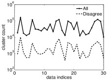
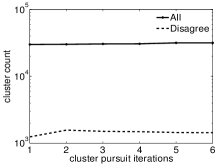
Figure 1: “stealth” clusters (solid) v.s. disagreeing “stealth” clusters (dashed) on dataset sidechain. Left: cluster pursuit for the first time for all problems (alphabetically sorted). Right: multiple cluster pursuits on problem 1qb7.

3.5 “Stealth” Cluster Pursuit

If GDD does not find the exact solution, then there exists a gap between the dual objective of GDD and the decoded primal objective. Various approaches, including (Komodakis and Paragios, 2008; Werner, 2008; Sontag et al, 2008; Batra et al, 2011), try to tighten the gap. These approaches typically involve two steps: 1) creating a dictionary of clusters, and then 2) search for a best cluster in the dictionary w.r.t. some score function. They typically use a fixed dictionary of clusters. For example, Sontag et al (2008) consider the dictionary as all possible triplets; Werner (2008) considers all order 4 cycles for grids type graphs.

Dual decrease is a popular choice of the score function. For example, Sontag et al (2008), brutal force search over the dictionary for the cluster with maximum dual decrease. Batra et al (2011) accelerate the process by computing primal dual gap for all clusters in the dictionary first (computing primal dual gap is much cheaper than computing dual decrease), and then only search over the clusters with non-zero primal dual gaps for the cluster with maximum dual decrease.

In this section, we show a new cluster pursuit strategy, which dynamically generates a dictionary of clusters instead of using a fixed one. The new cluster pursuit strategy is based on a special type of cluster which we call “stealth” clusters.

Definition 1 (“Stealth” cluster)

$\forall c_{1},c_{2}\in\operatorname{\mathcal{C}}^{\prime}$, we say $c=c_{1}\cup c_{2}$ is a “stealth” cluster if

1. $\exists s\in\operatorname{\mathcal{T}}$ s.t. $s\in\operatorname{\mathcal{S}}(c_{1})\setminus\{c_{1}\},s\in\operatorname{\mathcal{S}}(c_{2})\setminus\{c_{2}\}$, and

2. $\nexists\hat{c}\in\operatorname{\mathcal{C}}^{\prime}$ s.t. $c_{1}\in\operatorname{\mathcal{S}}(\hat{c})\setminus\{\hat{c}\},c_{2}\in\operatorname{\mathcal{S}}(\hat{c})\setminus\{\hat{c}\}$.

Proposition 4 essentially says there exist two maximisers that agree on $\operatorname{\mathbf{x}}_{s}$. There is however a situation where the decoding from different clusters may disagree. Let us consider two clusters $c_{1},c_{2}$ in Definition 1. According to Proposition 4 there exists a maximiser $\operatorname{\mathbf{x}}_{s}^{\prime}$ of $b_{s}(\operatorname{\mathbf{x}}_{s})$ that agrees with $b_{c_{1}}(\operatorname{\mathbf{x}}_{c_{1}})$, and a maximiser $\operatorname{\mathbf{x}}_{s}^{\prime\prime}$ of $b_{s}(\operatorname{\mathbf{x}}_{s})$ that agrees with $b_{c_{2}}(\operatorname{\mathbf{x}}_{c_{2}})$. However, if $b_{s}(\operatorname{\mathbf{x}}_{s})$ has multiple maximisers, the maximisers $\operatorname{\mathbf{x}}_{s}^{\prime}$ and $\operatorname{\mathbf{x}}_{s}^{\prime\prime}$ could be different. This means $b_{c_{1}}(\operatorname{\mathbf{x}}_{c_{1}})$ and $b_{c_{2}}(\operatorname{\mathbf{x}}_{c_{2}})$ may disagree on their overlap. Adding $c_{1}\cup c_{2}$ into $\operatorname{\mathcal{C}}^{\prime}$ with $\operatorname{\mathcal{S}}(c_{1}\cup c_{2})=\{s|s\in\operatorname{\mathcal{T}},s\subset(c_{1}\cup c_{2})\}$ at least one maximiser of $b_{c_{1}}(\operatorname{\mathbf{x}}_{c_{1}})$ and $b_{c_{2}}(\operatorname{\mathbf{x}}_{c_{2}})$ will become the same according to Proposition 4. This observation yields a strategy to dynamically generate dictionary of clusters to tighten the relaxation.

With similar derivation as in Sontag et al (2008), adding a new “stealth” cluster $c=c_{1}\cup c_{2}$ with $\operatorname{\mathcal{S}}(c)=\{s|s\in\operatorname{\mathcal{T}},s\subset c\}$, the dual decrease after one message updating for $c$ is

$$d_{1}(c)= g_{c}(\operatorname{\boldsymbol{\lambda}}_{c,\operatorname{\mathcal{S}}(c)})-g_{c}(\operatorname{\boldsymbol{\lambda}}^{*}_{c,\operatorname{\mathcal{S}}(c)})$$

$$= \sum_{s\in\mathcal{S}(c)\setminus\{c\}}\max_{\operatorname{\mathbf{x}}_{s}}b_{s}(\operatorname{\mathbf{x}}_{s})-\max_{\operatorname{\mathbf{x}}_{c}}\sum_{s\in\mathcal{S}(c)\setminus\{c\}}b_{s}(\operatorname{\mathbf{x}}_{s}).$$ (67)

In practice, we add clusters that will lead to largest dual decrease. With these observations, a new cluster pursuit strategy, which we call “stealth” cluster pursuit strategy, is summarised in Algorithm 3.

input :  $G=(\operatorname{\mathcal{V}},\operatorname{\mathcal{C}})$, $\operatorname{\mathcal{M}}_{L}(G,\operatorname{\mathcal{C}}^{\prime},\operatorname{\mathcal{S}}(\operatorname{\mathcal{C}}^{\prime}))$, $\operatorname{\mathcal{C}}^{\prime}$, $\operatorname{\mathcal{S}}(\operatorname{\mathcal{C}}^{\prime})$, $\boldsymbol{\theta}$,

threshold $T_{g},T_{a}$, max iterations $K^{1}_{max}$ and $K^{2}_{max}$,

max running time$\mathscr{T}_{max}$, cluster addition size $n$

output : $\operatorname{\mathbf{x}}^{*}$

1 $l=0$;

2 Initialise $\boldsymbol{\lambda}^{0}=\mathbf{0}$; $\operatorname{\mathbf{b}}^{0}:=(b^{0}_{t}(\operatorname{\mathbf{x}}_{t}))_{t\in\operatorname{\mathcal{T}}}=(\hat{\theta}_{t}(\operatorname{\mathbf{x}}_{t}))_{t\in\operatorname{\mathcal{T}}}$;

3 repeat

4       $l=l+1$; $\operatorname{\mathcal{T}}=\operatorname{\mathcal{C}}^{\prime}\cup(\cup_{c\in\operatorname{\mathcal{C}}^{\prime}}\operatorname{\mathcal{S}}(c))$; $\mathcal{P}=\emptyset$;

5       $K=\mathbbm{1}(l=1)K^{1}_{max}+\mathbbm{1}(l>1)K^{2}_{max}$;

6       Run Algo. 1 $(\boldsymbol{\lambda}^{l},\operatorname{\mathbf{b}}^{l})=$GDD$(G,\operatorname{\mathcal{M}}_{L},\operatorname{\mathcal{C}}^{\prime},\operatorname{\mathcal{S}}(\operatorname{\mathcal{C}}^{\prime}),\boldsymbol{\theta},T_{g},K,\boldsymbol{\lambda}^{l-1})$;

7       or Algo. 2 $\operatorname{\mathbf{b}}^{l}=$BP$(G,\operatorname{\mathcal{M}}_{L},\operatorname{\mathcal{C}}^{\prime},\operatorname{\mathcal{S}},\boldsymbol{\theta},T_{g},K,\operatorname{\mathbf{b}}^{l-1})$;

8      

9      for $t\in\operatorname{\mathcal{T}}$ do

10             for $c_{1},c_{2}\in\{c|c\in\operatorname{\mathcal{C}}^{\prime},t\in\operatorname{\mathcal{S}}(c)\setminus\{c\}\}$ do

11                   $\{\bar{\operatorname{\mathbf{x}}}_{c_{1}}\}=\mathop{\mathrm{argmax}}_{\operatorname{\mathbf{x}}_{c_{1}}}b^{l}_{c_{1}}(\operatorname{\mathbf{x}}_{c_{1}})$;

12                   $\{\hat{\operatorname{\mathbf{x}}}_{c_{2}}\}=\mathop{\mathrm{argmax}}_{\operatorname{\mathbf{x}}_{c_{1}}}b^{l}_{c_{2}}(\operatorname{\mathbf{x}}_{c_{2}})$;

13                   if $\nexists\bar{\operatorname{\mathbf{x}}}_{c_{1}},\hat{\operatorname{\mathbf{x}}}_{c_{2}},~{}\mathrm{s.t.}~{}\hat{\operatorname{\mathbf{x}}}_{t}=\bar{\operatorname{\mathbf{x}}}_{t}$ then

14                         $\mathcal{P}=\mathcal{P}\cup\{c_{1}\cup c_{2}\}$;

15                         $\operatorname{\mathcal{S}}(c_{1}\cup c_{2})=\{s|s\in\operatorname{\mathcal{T}},s\subset(c_{1}\cup c_{2})\}$;

16                         Compute $d_{1}(c)$ according to (67);

17                        

18                  

19            

20      Add the $n$ clusters in $\mathcal{P}$ with largest $d_{1}(c)$ to $\mathcal{C}^{\prime}$;

21       For all new added $c$, $\forall s\in\operatorname{\mathcal{S}}(c)\setminus\{c\},\operatorname{\mathbf{x}}_{s},\lambda_{c\rightarrow s}^{l}(\operatorname{\mathbf{x}}_{s})=0$;

22       Decode $\operatorname{\mathbf{x}}^{*}$ using (57) or (58);

23       $g(\boldsymbol{\lambda})=\sum_{t\in\operatorname{\mathcal{T}}}\max_{\operatorname{\mathbf{x}}_{t}}b_{t}(\operatorname{\mathbf{x}}_{t})$;

24      

25until $|g(\boldsymbol{\lambda})-p(\operatorname{\mathbf{x}}^{*}|\boldsymbol{\theta})|\leqslant T_{a}$ or running time$>\mathscr{T}_{max}$;

26

Algorithm 3 GDD with “Stealth” Cluster Pursuit

In a nutshell, we search for disagreeing clusters which maximise the dual decrease. In the worst case, this can be slow if too many disagreeing “stealth” clusters exist. However, in practice it is very fast. As we can see from Figure 1, the number of disagreeing “stealth” clusters is far less (about $1\%$ to $10\%$) than the total number of “stealth” clusters, which leads to a significant speed up. More importantly, “stealth” cluster pursuit makes our feasible set tighter than that of LP relaxation in (12) and GMPLP, which in turn are tighter than Dual Decomposition Sontag et al (2011).

“Stealth” cluster pursuit may get bigger and bigger clusters which would become prohibitively expensive to solve. In our experiments, it’s always computationally affordable. When it isn’t, one can use low order terms to approximate $b_{t}$. Furthermore both the frustrated cycle search strategy in Sontag et al (2012) and acceleration via evaluating primal dual gap first in Batra et al (2011) are applicable to GDD as well.

Convergence and Consistency

“Stealth” cluster pursuit can be seen as adding new constraints only. No matter which clusters are added to $\operatorname{\mathcal{C}}^{\prime}$, the dual decrease $d_{1}(c)$ is always no-negative. Thus GDD with “stealth” cluster pursuit still have the same convergence and consistency properties as original GDD presented in Section 3.3.2.

4 Marginal Polytope Diagrams

LP relaxation based message passings can be slow if there are too many constraints. This motivates us to seek ways of reducing the number of constraints to reduce computational complexity without sacrificing the quality of the solution. Here we first propose a new tool which we call marginal polytope diagrams. Then with this tool, we show how to reduce constraints without loosening the optimisation problem.

Definition 2 (Marginal Polytope Diagram)

Given a graph $G=(\operatorname{\mathcal{V}},\operatorname{\mathcal{C}})$, $G^{M}=(\operatorname{\mathcal{V}}^{M},\operatorname{\mathcal{E}}^{M})$ with node set $\operatorname{\mathcal{V}}^{M}$ and edge set $\operatorname{\mathcal{E}}^{M}$ is said to be a marginal polytope diagram of $G$ if

1. $\operatorname{\mathcal{C}}\subseteq\operatorname{\mathcal{V}}^{M}\subseteq 2^{\operatorname{\mathcal{V}}}$ and

2. a directed edge from $c$ to $s$ deonted by $(c\rightarrow s)$, belongs to $\operatorname{\mathcal{E}}^{M}$ only nodes if $c,s\in\operatorname{\mathcal{V}}^{M},~{}s\subseteq c$.

Remarks

Previous work in this vein includes Region graphs Yedidia et al (2005); Koller and Friedman (2009) and Hasse diagrams (a.k.a poset diagrams) Pakzad and Anantharam (2005); Wainwright and Jordan (2008); McEliece and Yildirim (2003). What distinguishes marginal polytope diagrams, however, is the fact that the receivers of an edge can be a subset of the senders, where Region graphs and Hasse diagrams require that the edge’s receivers must be a proper subset of the senders. For example, the definition of region graph in Page 419 of (Koller and Friedman, 2009), requires that a receiver must be a proper subset of a sender in region graph. Likewise in Page 16 of (Yedidia et al, 2005), the authors state that a region graph must be a directed acyclic graph, which means that the edge’s receivers must be a proper subset of the senders (otherwise there would be a loop from a region to itself). This is particularly significant since some dual message passing algorithms (including GMPLP) send messages from a cluster $c$ to itself. Hasse diagrams Pakzad and Anantharam (2005) have a further restriction, which corresponds to a special case of Marginal Polytope Diagram, where for arbitrary $v_{1},v_{2}\in\operatorname{\mathcal{V}}^{M},v_{1}\subset v_{2}$ edge $(v_{1}\rightarrow v_{2})\in\operatorname{\mathcal{E}}^{M}$ if and only if $\nexists v_{3}\in\operatorname{\mathcal{V}}^{M}$, s.t. $v_{2}\subset v_{3}\subset v_{1}$. In some LP relaxation based message passing algorithms, some local marginalisation constraints from a cluster to itself are required, thus violating the proper subset requirement. Both Hasse diagrams and Region graphs are inapplicable in this case. For example, in Section 6 of Globerson and Jaakkola (2007), GMPLP sends messages from one cluster to itself, which requires a local marginalisation constraint from one cluster to itself. In Sontag et al (2008), the message $\lambda_{ij\to ij}$ (in their Figure 1) is from the edge $ij$ to itself, which requires a local marginalisation constraint from the edge to itself. The proposed marginal polytope diagram not only handles the above situations, but also provides a natural correspondence among marginal polytope diagram, local marginal polytope and MAP message passing.

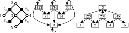
Figure 2: An example of marginal polytope diagram. Left: a factor graph $G=(\operatorname{\mathcal{V}},\operatorname{\mathcal{C}})$ with $\operatorname{\mathcal{V}}=\{1,2,3,4,5\}$ and $\operatorname{\mathcal{C}}=\{c_{1},c_{2},c_{3},c_{4}\}$, where $c_{1}=\{1,2,3\},~{}c_{2}=\{2,3,4\}$, $c_{3}=\{3,4,5\}$ and $c_{4}=\{3\}$. Middle: a marginal polytope diagram associated with the local marginal polytope $\operatorname{\mathcal{M}}_{L}(G,\operatorname{\mathcal{C}},\operatorname{\mathcal{S}}_{g}(\operatorname{\mathcal{C}}))$ in GMPLP. Right: a marginal polytope diagram associated with the local marginal polytope $\operatorname{\mathcal{M}}_{L}(G,\operatorname{\mathcal{C}},\operatorname{\mathcal{S}}_{d}(\operatorname{\mathcal{C}}))$ in dual decomposition.

In marginal polytope diagrams, we use rectangles to represent nodes (to differentiate from a graph of graphical models) similar to Hasse diagrams (see Section 4.2.1 in Wainwright and Jordan (2008)). An example is given in Figure 2. For the marginal polytope diagram associated with GMPLP (in Figure 2 middle) has edges from a node to itself, which are not allowed in both Region graphs and Hasse diagrams. Also edges like $(\{2,3,4\}\rightarrow\{3\})$ are not allowed in Hasse diagrams. We choose to use the term diagram instead of graph in order to distinguish from graphs in graphical models.

From local marginal polytope to diagram

Given a graph $G=(\operatorname{\mathcal{V}},\operatorname{\mathcal{C}})$ and arbitrary local marginal polytope $\operatorname{\mathcal{M}}_{L}(G,\operatorname{\mathcal{C}}^{\prime},\operatorname{\mathcal{S}}(\operatorname{\mathcal{C}}^{\prime}))$, the corresponding marginal polytope diagram $G^{M}=(\operatorname{\mathcal{V}}^{M},\operatorname{\mathcal{E}}^{M})$ can be constructed as:

1. $\operatorname{\mathcal{V}}^{M}=\operatorname{\mathcal{T}}$ ($\operatorname{\mathcal{T}}$ is defined in (47)),

2. $\forall c\in\operatorname{\mathcal{C}}^{\prime},$ if $s\in\operatorname{\mathcal{S}}(c)$, then $(c\rightarrow s)\in\operatorname{\mathcal{E}}^{M}$.

From diagram to local marginal polytope

Given a graph $G=(\operatorname{\mathcal{V}},\operatorname{\mathcal{C}})$ and a marginal polytope diagram $G^{M}=(\operatorname{\mathcal{V}}^{M},\operatorname{\mathcal{E}}^{M})$, the corresponding local marginal polytope $\operatorname{\mathcal{M}}_{L}(G,\operatorname{\mathcal{C}}^{\prime},\operatorname{\mathcal{S}}(\operatorname{\mathcal{C}}^{\prime}))$ can be recovered as follows:

$$\operatorname{\mathcal{C}}^{\prime} =\{c|c\in\operatorname{\mathcal{V}}^{M},\exists(c\rightarrow s)\in\operatorname{\mathcal{E}}^{M}\},$$

$$\operatorname{\mathcal{S}}(c) =\{s|(c\rightarrow s)\in\operatorname{\mathcal{E}}^{M}\},\forall c\in\operatorname{\mathcal{C}}^{\prime}.$$ (68)

4.1 Equivalent Edges

Definition 3 (Edge equivalence)

For arbitrary $G=(\operatorname{\mathcal{V}},\operatorname{\mathcal{C}})$, and marginal polytope diagram $G^{M}=(\operatorname{\mathcal{V}}^{M},\operatorname{\mathcal{E}}^{M})$ of $G$, $\forall c_{1},c_{2},t\in\operatorname{\mathcal{V}}^{M},t\subseteq c_{1},t\subseteq c_{2}$, given

$$\operatorname{\mathcal{U}}=\big{\{} \sum_{\operatorname{\mathbf{x}}_{c\setminus s}}\mu_{c}(\operatorname{\mathbf{x}}_{c})=\mu_{s}(\operatorname{\mathbf{x}}_{s}),\forall(c\rightarrow s)\in$$

$$(\operatorname{\mathcal{E}}^{M}\setminus\{(\hat{c}\rightarrow t)|\hat{c}\in\operatorname{\mathcal{V}}^{M},t\subseteq\hat{c}\}),\operatorname{\mathbf{x}}_{s}\big{\}},$$ (69)

edges $(c_{1}\rightarrow t)$ and $(c_{2}\rightarrow t)$ are said to be equivalent w.r.t $G^{M}$ denoted by $(c_{1}\rightarrow t)\Leftrightarrow(c_{2}\rightarrow t)$, if the following holds:

$$\Big{\{}\operatorname{\boldsymbol{\mu}}|\operatorname{\mathcal{U}}\cup\{\sum_{\operatorname{\mathbf{x}}_{c_{1}\setminus t}}\mu_{c_{1}}(\operatorname{\mathbf{x}}_{c_{1}})=\mu_{t}(\operatorname{\mathbf{x}}_{t}),\forall\operatorname{\mathbf{x}}_{t}\}\Big{\}}$$

$$= \Big{\{}\operatorname{\boldsymbol{\mu}}|\operatorname{\mathcal{U}}\cup\{\sum_{\operatorname{\mathbf{x}}_{c_{2}\setminus t}}\mu_{c_{2}}(\operatorname{\mathbf{x}}_{c_{2}})=\mu_{t}(\operatorname{\mathbf{x}}_{t}),\forall\operatorname{\mathbf{x}}_{t}\}\Big{\}}.$$ (70)

Note that the definition of edge equivalence does not require $(c_{1}\rightarrow t)$ and $(c_{2}\rightarrow t)$ from $\operatorname{\mathcal{E}}^{M}$. Checking whether two edges are equivalent via Definition 3 might be inconvenient. In fact, edge equivalence can be read directly from a marginal polytope diagram.

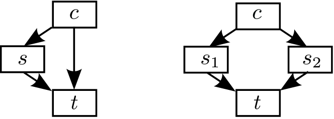
Figure 3: Two types of edge equivalence in Proposition 7. Left: Type 1 $(c\rightarrow t)\Leftrightarrow(s\rightarrow t)$. Right: Type 2 $(s_{1}\rightarrow t)\Leftrightarrow(s_{2}\rightarrow t)$.

Figure 4: A counter example for the simpler edge equivalence definition.

Proposition 7

Given a graph $G=(\operatorname{\mathcal{V}},\operatorname{\mathcal{C}})$ and a marginal polytope diagram $G^{M}=(\operatorname{\mathcal{V}}^{M},\operatorname{\mathcal{E}}^{M})$ of $G$, we have

1. $\forall c,s,t\in\operatorname{\mathcal{V}}^{M}$, $t\subset s\subset c$, if $(c\rightarrow s)\in\operatorname{\mathcal{E}}^{M}$, then $(c\rightarrow t)\Leftrightarrow(s\rightarrow t)$;

2. If $(c\rightarrow s_{1}),(c\rightarrow s_{2})\in\operatorname{\mathcal{E}}^{M}$, then $\forall t\in\operatorname{\mathcal{V}}^{M},t\subset s_{1},t\subset s_{2}$, $(s_{1}\rightarrow t)\Leftrightarrow(s_{2}\rightarrow t)$.

The proof is provided in Section LABEL:sec:Proofofeqedge of supplementary. In Figure 4 we give examples of the two types of edge equivalence in Proposition 7. Furthermore, the following proposition always holds.

Proposition 8

For arbitrary $G=(\operatorname{\mathcal{V}},\operatorname{\mathcal{C}})$, and marginal polytope diagram $G^{M}=(\operatorname{\mathcal{V}}^{M},\operatorname{\mathcal{E}}^{M})$ of $G$, edge equivalence w.r.t. $G^{M}$ is an equivalence relation.

The proof is provided in Section LABEL:sec:proof_equi_relation of supplementary.

Simpler edge equivalence definition?

Readers may wonder why in Definition 3, all edges sent to $t$ are removed (see (69)), instead of only removing two edges $(c_{1}\rightarrow t),(c_{2}\rightarrow t)$. The answer is that if we did so, the resulting edge equivalence (we call it simpler edge equivalence) would no longer be an equivalence relation. To see this, we can replace $\operatorname{\mathcal{E}}^{M}\setminus\{(\hat{c}\rightarrow t)|\hat{c}\in\operatorname{\mathcal{V}}^{M}\}$ with $\operatorname{\mathcal{E}}^{M}\setminus\{(c_{1}\rightarrow t),(c_{2}\rightarrow t)\}$ in (69), and see a counter example in Figure 4. In considering whether $(s_{1}\rightarrow t)\notin\operatorname{\mathcal{E}}^{M}$ and $(s_{4}\rightarrow t)\notin\operatorname{\mathcal{E}}^{M}$ are equivalent, we need to consider two constraint sets $\operatorname{\mathcal{U}}_{a}=\{\sum_{\operatorname{\mathbf{x}}_{c\setminus s}}\mu_{c}(\operatorname{\mathbf{x}}_{c})=\mu_{s}(\operatorname{\mathbf{x}}_{s}),\forall(c\rightarrow s)\in\operatorname{\mathcal{E}}^{M}\cup\{(s_{1}\rightarrow t)\},\operatorname{\mathbf{x}}_{s}\}$ and $\operatorname{\mathcal{U}}_{b}=\{\sum_{\operatorname{\mathbf{x}}_{c\setminus s}}\mu_{c}(\operatorname{\mathbf{x}}_{c})=\mu_{s}(\operatorname{\mathbf{x}}_{s}),\forall(c\rightarrow s)\in\operatorname{\mathcal{E}}^{M}\cup\{(s_{4}\rightarrow t)\},\operatorname{\mathbf{x}}_{s}\}$. Then by the fact $(s_{1}\rightarrow t)\Leftrightarrow(s_{2}\rightarrow t)$, $(s_{3}\rightarrow t)\Leftrightarrow(s_{4}\rightarrow t)$, $(s_{2}\rightarrow t)\in\operatorname{\mathcal{E}}^{M},(s_{3}\rightarrow t)\in\operatorname{\mathcal{E}}^{M}$, we have $\{\operatorname{\boldsymbol{\mu}}|\operatorname{\mathcal{U}}_{a}\}=\{\operatorname{\boldsymbol{\mu}}|\operatorname{\mathcal{U}}_{b}\}$. Thus $(s_{1}\rightarrow t)\Leftrightarrow(s_{4}\rightarrow t)$ by the simpler edge equivalence definition. However, by the simpler edge equivalence definition $(s_{2}\rightarrow t)$, $(s_{3}\rightarrow t)$ are not equivalent in general. This means transitivity does not hold. Thus the simpler edge equivalence is not an equivalence relation. Figure 4 is not a counter example for Definition 3, because $(s_{1}\rightarrow t)$, $(s_{4}\rightarrow t)$ are not equivalent by Definition 3.

With edge equivalence, we can see that given a marginal polytope diagram $G^{M}=(\operatorname{\mathcal{V}}^{M},\operatorname{\mathcal{E}}^{M})$ of a graph $G=(\operatorname{\mathcal{V}},\operatorname{\mathcal{C}})$, the following two operations would not change the corresponding local marginal polytope.

1. Adding a new edge that is equivalent to an existing edge in $\operatorname{\mathcal{E}}^{M}$ ;

2. Removing one of two existing equivalent edges in $\operatorname{\mathcal{E}}^{M}$.

By composing the two operations above, we are able to derive a series of operations which would not change the corresponding local marginal polytope. For illustration, using Operation 1) first and then using Operation 2) would lead to an operation: replacing an existing edge in $\operatorname{\mathcal{E}}^{M}$ with an equivalent edge. Repeating Operation 2) we can merge several equivalent edges in $\operatorname{\mathcal{E}}^{M}$ to one edge. Repeating Operation 2) and then using Operation 1) we can replace a group of equivalent edges in $\operatorname{\mathcal{E}}^{M}$ with a new equivalent edge.

4.2 Redundant Nodes

There is a type of node, the removal of which from a marginal polytope diagram does not change the local marginal polytope.

Definition 4 (Redundant Node)

For any graph $G=(\operatorname{\mathcal{V}},\operatorname{\mathcal{C}})$, and marginal polytope diagram $G^{M}=(\operatorname{\mathcal{V}}^{M},\operatorname{\mathcal{E}}^{M})$ of $G$, we say $v\in\operatorname{\mathcal{V}}^{M}\setminus\operatorname{\mathcal{C}}$ is a redundant node w.r.t. $G^{M}$, if

$$\Big{\{}\operatorname{\boldsymbol{\mu}}|\sum_{\operatorname{\mathbf{x}}_{c\setminus s}}\mu_{c}(\operatorname{\mathbf{x}}_{c})=\mu_{s}(\operatorname{\mathbf{x}}_{s}),\forall(c\rightarrow s)\in\operatorname{\mathcal{E}}^{M},\operatorname{\mathbf{x}}_{s}\Big{\}}$$

$$= \Big{\{}\operatorname{\boldsymbol{\mu}}|\sum_{\operatorname{\mathbf{x}}_{c\setminus s}}\mu_{c}(\operatorname{\mathbf{x}}_{c})=\mu_{s}(\operatorname{\mathbf{x}}_{s}),\forall(c\rightarrow s)\in\hat{\operatorname{\mathcal{E}}}^{M},\operatorname{\mathbf{x}}_{s}\Big{\}}$$

where

$$\hat{\operatorname{\mathcal{E}}}^{M}= \Big{[}\operatorname{\mathcal{E}}^{M}\setminus(\{(c\rightarrow v)\in\operatorname{\mathcal{E}}^{M}\}\cup\{(v\rightarrow s)\in\operatorname{\mathcal{E}}^{M}\})\Big{]}$$

$$\cup\Big{\{}(c\rightarrow s)|(c\rightarrow v)\in\operatorname{\mathcal{E}}^{M},(v\rightarrow s)\in\operatorname{\mathcal{E}}^{M}\Big{\}}.$$

The following proposition provides an easy way to find redundant nodes in a marginal polytope diagram.

Proposition 9

Given a graph $G=(\operatorname{\mathcal{V}},\operatorname{\mathcal{C}})$ and a marginal polytope diagram $G^{M}=(\operatorname{\mathcal{V}}^{M},\operatorname{\mathcal{E}}^{M})$, $v\in\operatorname{\mathcal{V}}^{M}\setminus\operatorname{\mathcal{C}}$ is a redundant node w.r.t. $G^{M}$ if either of the following statements is true:

1. There is only one $(c\rightarrow v)\in\operatorname{\mathcal{E}}^{M}$;

2. All $(c\rightarrow v)\in\operatorname{\mathcal{E}}^{M}$ are equivalent w.r.t. $G^{M}$ according to Definition 3.

Proof

Let us consider the first case where there is only one $(c\rightarrow v)\in\operatorname{\mathcal{E}}^{M}$. It is easy to check that

$$\left\{\operatorname{\boldsymbol{\mu}}\left|\begin{array}[]{l}\forall(v\rightarrow s)\in\operatorname{\mathcal{E}}^{M},\operatorname{\mathbf{x}}_{s},\sum\limits_{\operatorname{\mathbf{x}}_{c\setminus s}}\mu_{c}(\operatorname{\mathbf{x}}_{c})=\mu_{s}(\operatorname{\mathbf{x}}_{s});\\ \forall\operatorname{\mathbf{x}}_{v},~{}~{}\sum\limits_{\operatorname{\mathbf{x}}_{c\setminus v}}\mu_{c}(\operatorname{\mathbf{x}}_{c})=\mu_{v}(\operatorname{\mathbf{x}}_{v})\end{array}\right.\right\}$$ (71c)

$$=\left\{\operatorname{\boldsymbol{\mu}}\left|\begin{array}[]{l}\forall\operatorname{\mathbf{x}}_{v},~{}\sum\limits_{\operatorname{\mathbf{x}}_{c\setminus v}}\mu_{c}(\operatorname{\mathbf{x}}_{c})=\mu_{v}(\operatorname{\mathbf{x}}_{v});\\ \forall(v\rightarrow s)\in\operatorname{\mathcal{E}}^{M},\operatorname{\mathbf{x}}_{s},~{}\sum\limits_{\operatorname{\mathbf{x}}_{v\setminus s}}\mu_{v}(\operatorname{\mathbf{x}}_{v})=\mu_{s}(\operatorname{\mathbf{x}}_{s})\end{array}\right.\right\}.$$ (71f)

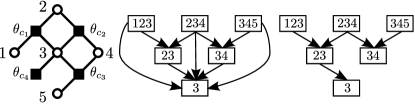
Figure 5: An example of equivalent edges removal. Left: a factor graph $G=(\operatorname{\mathcal{V}},\operatorname{\mathcal{C}})$ with $\operatorname{\mathcal{V}}=\{1,2,3,4,5\}$ and $\operatorname{\mathcal{C}}=\{c_{1},c_{2},c_{3},c_{4}\}$, where $c_{1}=\{1,2,3\},~{}c_{2}=\{2,3,4\}$, $c_{3}=\{3,4,5\}$ and $c_{4}=\{3\}$. Middle: a marginal polytope diagram whose edges $(\{1,2,3\}\rightarrow\{3\})$,$(\{2,3,4\}\rightarrow\{3\})$, $(\{3,4,5\}\rightarrow\{3\})$,$(\{2,3\}\rightarrow\{3\})$ and $(\{3,4\}\rightarrow\{3\})$ are equivalent. Right: a marginal polytope diagram after removal of equivalent edges.

Since $v\notin\operatorname{\mathcal{C}}$, $\mu_{v}(\operatorname{\mathbf{x}}_{v})$ is not part of $\operatorname{\boldsymbol{\mu}}$ in (3). Note that removing $\sum_{\operatorname{\mathbf{x}}_{c\setminus v}}\mu_{c}(\operatorname{\mathbf{x}}_{c})=\mu_{v}(\operatorname{\mathbf{x}}_{v}),~{}\forall\operatorname{\mathbf{x}}_{v}$ from (71c) would not change the set of $\operatorname{\boldsymbol{\mu}}$ described by (71c) as no other variables depend on $\mu_{v}(\operatorname{\mathbf{x}}_{v})$. That is,

$$\Big{\{}\operatorname{\boldsymbol{\mu}}|\sum_{\operatorname{\mathbf{x}}_{\hat{c}\setminus\hat{s}}}\mu_{\hat{c}}(\operatorname{\mathbf{x}}_{\hat{c}})=\mu_{\hat{s}}(\operatorname{\mathbf{x}}_{\hat{s}}),\forall(\hat{c}\rightarrow\hat{s})\in\operatorname{\mathcal{E}}^{M}_{1},\operatorname{\mathbf{x}}_{\hat{s}}\Big{\}}$$

$$= \Big{\{}\operatorname{\boldsymbol{\mu}}|\sum_{\operatorname{\mathbf{x}}_{\hat{c}\setminus\hat{s}}}\mu_{\hat{c}}(\operatorname{\mathbf{x}}_{\hat{c}})=\mu_{\hat{s}}(\operatorname{\mathbf{x}}_{\hat{s}}),\forall(\hat{c}\rightarrow\hat{s})\in\operatorname{\mathcal{E}}^{M}_{2},\operatorname{\mathbf{x}}_{\hat{s}}\Big{\}},$$

where $\operatorname{\mathcal{E}}^{M}_{1}=\{(c\rightarrow s)|(v\rightarrow s)\in\operatorname{\mathcal{E}}^{M}\}$, and $\operatorname{\mathcal{E}}^{M}_{2}=\{(c\rightarrow v)\}\cup\{(v\rightarrow s)\in\operatorname{\mathcal{E}}^{M}\}$. Let $A=\{\operatorname{\boldsymbol{\mu}}|\sum_{\operatorname{\mathbf{x}}_{\hat{c}\setminus\hat{s}}}\mu_{\hat{c}}(\operatorname{\mathbf{x}}_{\hat{c}})=\mu_{\hat{s}}(\operatorname{\mathbf{x}}_{\hat{s}}),\forall(\hat{c}\rightarrow\hat{s})\in\operatorname{\mathcal{E}}^{M}\setminus\operatorname{\mathcal{E}}^{M}_{2},\operatorname{\mathbf{x}}_{\hat{s}}\}.$ We have

$$\Big{\{}\operatorname{\boldsymbol{\mu}}|\sum_{\operatorname{\mathbf{x}}_{\hat{c}\setminus\hat{s}}}\mu_{\hat{c}}(\operatorname{\mathbf{x}}_{\hat{c}})=\mu_{\hat{s}}(\operatorname{\mathbf{x}}_{\hat{s}}),\forall(\hat{c}\rightarrow\hat{s})\in\operatorname{\mathcal{E}}^{M}_{1},\operatorname{\mathbf{x}}_{\hat{s}}\Big{\}}\cap A$$

$$= \Big{\{}\operatorname{\boldsymbol{\mu}}|\sum_{\operatorname{\mathbf{x}}_{\hat{c}\setminus\hat{s}}}\mu_{\hat{c}}(\operatorname{\mathbf{x}}_{\hat{c}})=\mu_{\hat{s}}(\operatorname{\mathbf{x}}_{\hat{s}}),\forall(\hat{c}\rightarrow\hat{s})\in\operatorname{\mathcal{E}}^{M}_{2},\operatorname{\mathbf{x}}_{\hat{s}}\Big{\}}\cap A.$$

Since ${\operatorname{\mathcal{E}}}^{M}=(\operatorname{\mathcal{E}}^{M}\setminus\operatorname{\mathcal{E}}^{M}_{2})\cup\operatorname{\mathcal{E}}^{M}_{2}$ and $\hat{\operatorname{\mathcal{E}}}^{M}=(\operatorname{\mathcal{E}}^{M}\setminus\operatorname{\mathcal{E}}^{M}_{2})\cup\operatorname{\mathcal{E}}^{M}_{1}$,

$$\Big{\{}\operatorname{\boldsymbol{\mu}}|\sum_{\operatorname{\mathbf{x}}_{\hat{c}\setminus\hat{s}}}\mu_{\hat{c}}(\operatorname{\mathbf{x}}_{\hat{c}})=\mu_{\hat{s}}(\operatorname{\mathbf{x}}_{\hat{s}}),\forall(\hat{c}\rightarrow\hat{s})\in\hat{\operatorname{\mathcal{E}}}^{M},\operatorname{\mathbf{x}}_{\hat{s}}\Big{\}}$$

$$= \Big{\{}\operatorname{\boldsymbol{\mu}}|\sum_{\operatorname{\mathbf{x}}_{\hat{c}\setminus\hat{s}}}\mu_{\hat{c}}(\operatorname{\mathbf{x}}_{\hat{c}})=\mu_{\hat{s}}(\operatorname{\mathbf{x}}_{\hat{s}}),\forall(\hat{c}\rightarrow\hat{s})\in\operatorname{\mathcal{E}}^{M},\operatorname{\mathbf{x}}_{\hat{s}}\Big{\}}.$$

Hence $v$ is a redundant node by definition.

Now let us consider the second case, where there are multiple equivalent $(c\rightarrow v)\in\operatorname{\mathcal{E}}^{M}$. By edge equivalence we can keep one of $(c\rightarrow v)\in\operatorname{\mathcal{E}}^{M}$ and remove the rest without changing the local marginal polytope, which becomes the first case.

5 Constraint Reduction

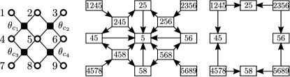
Figure 6: An example of redundant node removal. Left: a factor graph $G=(\operatorname{\mathcal{V}},\operatorname{\mathcal{C}})$ with $\operatorname{\mathcal{V}}=\{1,2,3,4,5,6,7,8,9\}$, and $\operatorname{\mathcal{C}}=\{c_{1},c_{2},c_{3},c_{4}\}$, where $c_{1}=\{1,2,4,5\},~{}c_{2}=\{2,3,5,6\},~{}c_{3}=\{4,5,7,8\}$, and $c_{4}=\{5,6,8,9\}$. Middle: a marginal polytope diagram with redundant nodes $\{2,4,5\}$, $\{2,5,6\}$, $\{4,5,8\}$, $\{5,6,8\}$ and $\{5\}$. Right: marginal polytope diagram after redundant nodes removal.

Equivalent edges offer an effective way to reduce constraints. By composing the two basic operations in Section 4.1, we can get a series of operations which would not change the corresponding local marginal polytope. For illustration we can partition $\operatorname{\mathcal{E}}^{M}$ into several equivalent classes by equivalence between edges, and we can simply pick up arbitrarily many edges in each equivalent class to get a new marginal polytope diagram with fewer edges. As each edge corresponds to a local marginalisation constraint, the number of constraints can be efficiently reduced by the above operations. As shown in Figure 5, all edges to node $\{3\}$ are equivalent, thus we can keep just one of them in the diagram to keep the local marginal polytope unaltered yet with fewer constraints.

Given a graph $G=(\operatorname{\mathcal{V}},\operatorname{\mathcal{C}})$, and a marginal polytope diagram $G^{M}=(\operatorname{\mathcal{V}}^{M},\operatorname{\mathcal{E}}^{M})$ of $G$, if a node $v\in\operatorname{\mathcal{V}}^{M}$ is a redundant node, we can reduce the number of constraints by removing $v$ from $\operatorname{\mathcal{V}}^{M}$ to obtain a marginal polytope diagram as follows:

$$G^{M}_{R}= (\operatorname{\mathcal{V}}^{M}_{R},\operatorname{\mathcal{E}}^{M}_{R}),\operatorname{\mathcal{V}}^{M}_{R}=\operatorname{\mathcal{V}}^{M}\setminus\{v\},$$

$$\operatorname{\mathcal{E}}^{M}_{R}= [\operatorname{\mathcal{E}}^{M}\setminus(\{(c\rightarrow v)\in\operatorname{\mathcal{E}}^{M}\}\cup\{(v\rightarrow s)\in\operatorname{\mathcal{E}}^{M}\})]$$

$$\cup\{(c\rightarrow s)|(c\rightarrow v),(v\rightarrow s)\in\operatorname{\mathcal{E}}^{M}\},$$ (72)

and according to the definition of redundant nodes, $G^{M}_{R}$ and $G^{M}$ correspond to the same local marginal polytope.

Figure 6 gives an example of redundant node removal. In the middle diagram, one can see that nodes $\{2,4,5\}$, $\{2,5,6\}$, $\{4,5,8\}$, and $\{5,6,8\}$ are redundant because their indegrees are 1. For node $\{5\}$, as all edges to $\{5\}$ are equivalent, node $\{5\}$ is also redundant. Removal of these redundant nodes leads to fewer constraints without changing the local marginal polytope.

It is worth mentioning that Kolmogorov and Schoenemann (2012) is perhaps closest idea to ours in spirit. However, (Kolmogorov and Schoenemann, 2012, Proposition 2.1) considers the removal of edges only, whereas ours considers the removal of both edges and nodes.

5.1 Is the Minimal Number of Constraints Always a Good Choice?

Using marginal polytope diagrams one can safely reduce the number of constraints without altering the local marginal polytope. On one hand, fewer constraints means fewer belief updates on $b_{t}(\operatorname{\mathbf{x}}_{t}),t\in\operatorname{\mathcal{T}}$, which leads to lower run time per iteration. On the other hand, fewer constraints means fewer coordinates (i.e. search directions), and thus that the algorithm is more likely to get stuck at corners due to the non-smoothness of the dual objective and the nature of coordinate descent (this has been often observed empirically too). This means that minimal number of constraints is not always a good choice. As we shall see in the next section, a trade-off between the minimal number of constraints and the maximal number of constraints performs best.

6 From Constraint Reduction To New Message Passing Algorithms

Here we propose three new efficient algorithms for MAP inference, using different constraint reduction strategies (via marginal polytope diagrams). All three algorithms are based on the GDD belief propagation procedure which is equivalent to GDD message passing, thus the theoretical properties in Section 3.3.2 also hold for these three algorithms.

To derive new algorithms, we first construct a local marginal polytope as an initial local marginal polytope, and then by different constraint reduction strategies we get three different algorithms. For arbitrary graph $G=(\operatorname{\mathcal{V}},\operatorname{\mathcal{C}})$, we let $\operatorname{\mathcal{C}}^{\prime}$ be $\operatorname{\mathcal{C}}_{0}=\{c^{\prime}|c^{\prime}\subseteq c,c\in\operatorname{\mathcal{C}}\}$ and $\operatorname{\mathcal{S}}(\operatorname{\mathcal{C}}^{\prime})$ be $\operatorname{\mathcal{S}}_{0}(\operatorname{\mathcal{C}}_{0})=(\operatorname{\mathcal{S}}_{0}(c))_{c\in\operatorname{\mathcal{C}}_{0}}$ with $\operatorname{\mathcal{S}}_{0}(c)=\{s|s\in\operatorname{\mathcal{C}}_{0},s\subset c\}$ to construct a local marginal polytope $\operatorname{\mathcal{M}}_{L}(G,\operatorname{\mathcal{C}}_{0},\operatorname{\mathcal{S}}_{0}(\operatorname{\mathcal{C}}_{0}))$ as a initial local marginal polytope. Thus the marginal polytope diagram is $G^{M}_{0}=(\operatorname{\mathcal{V}}^{M}_{0},\operatorname{\mathcal{E}}^{M}_{0})$ where

$$\operatorname{\mathcal{V}}^{M}_{0} =\{v|v\subseteq c,c\in\operatorname{\mathcal{C}}\},$$

$$\operatorname{\mathcal{E}}^{M}_{0} =\{(c\rightarrow s)|c,s\in\operatorname{\mathcal{V}}^{M}_{0},s\subset c\}.$$ (73)

The marginal polytope diagram $G^{M}_{0}$ and GDD provide the base for all three algorithms.

6.1 Power Set Algorithm

In the first algorithm which we call Power Set algorithm, we do not remove any redundant nodes in $G^{M}_{0}$. One can see that $\forall(c\rightarrow t)\in\operatorname{\mathcal{E}}^{M}_{0},|c|-|t|>1$, $\exists s\in\operatorname{\mathcal{V}}^{M}_{0},s.t.|s|=|t|+1,(c\rightarrow s)\in\operatorname{\mathcal{E}}^{M}_{0}$, which suggests $(c\rightarrow t)\Leftrightarrow(s\rightarrow t)$. Using equivalent edges we get a marginal polytope diagram $G^{M}_{p}=(\operatorname{\mathcal{V}}^{M}_{p},\operatorname{\mathcal{E}}^{M}_{p})$ as follows

$$\operatorname{\mathcal{V}}^{M}_{p} =\operatorname{\mathcal{V}}^{M}_{0},$$

$$\operatorname{\mathcal{E}}^{M}_{p} =\{(c\rightarrow s)|c,s\in\operatorname{\mathcal{V}}^{M}_{p},s\subset c,|c|=|s|+1\},$$ (74)

which corresponds to the same local marginal polytope as $G^{M}_{0}$. Thus we define $\operatorname{\mathcal{C}}_{p}=\{c|c\subseteq\hat{c},\hat{c}\in\operatorname{\mathcal{C}}\}$, $\operatorname{\mathcal{S}}_{p}(c)=\{s|(c\rightarrow s)\in\operatorname{\mathcal{E}}^{M}_{p}\}$, and let $\operatorname{\mathcal{C}}^{\prime}$ be $\operatorname{\mathcal{C}}_{p}$, and $\operatorname{\mathcal{S}}(\operatorname{\mathcal{C}}^{\prime})$ be $\operatorname{\mathcal{S}}_{p}(\operatorname{\mathcal{C}}_{p})=(\operatorname{\mathcal{S}}_{p}(c))_{c\in\operatorname{\mathcal{C}}^{\prime}}$, the corresponding local marginal polytope becomes $\operatorname{\mathcal{M}}_{L}(G,\operatorname{\mathcal{C}}_{p},\operatorname{\mathcal{S}}_{p}(\operatorname{\mathcal{C}}_{p}))$. By the fact that $c\notin\operatorname{\mathcal{S}}_{p}(c),\forall c\in\operatorname{\mathcal{C}}_{p}$, applying belief propagation without messages to $\operatorname{\mathcal{M}}_{L}(G,\operatorname{\mathcal{C}}_{p},\operatorname{\mathcal{S}}_{p}(\operatorname{\mathcal{C}}_{p}))$ yields the following belief propagation form $\forall c\in\operatorname{\mathcal{C}}_{p}$:

$$b_{s}^{*}(\operatorname{\mathbf{x}}_{s}) =\frac{1}{|c|}\max_{\operatorname{\mathbf{x}}_{c\setminus s}}[b_{c}(\operatorname{\mathbf{x}}_{c})+\sum_{\hat{s}\in\operatorname{\mathcal{S}}_{p}(c)}b_{\hat{s}}(\operatorname{\mathbf{x}}_{\hat{s}})],\forall s\in\operatorname{\mathcal{S}}_{p}(c),\operatorname{\mathbf{x}}_{s}$$

$$b_{c}^{*}(\operatorname{\mathbf{x}}_{c}) =b_{c}(\operatorname{\mathbf{x}}_{c})+\sum_{\hat{s}\in\operatorname{\mathcal{S}}_{p}(c)}b_{\hat{s}}(\operatorname{\mathbf{x}}_{\hat{s}})-\sum_{\hat{s}\in\operatorname{\mathcal{S}}_{p}(c)}b_{\hat{s}}^{*}(\operatorname{\mathbf{x}}_{\hat{s}}),\forall\operatorname{\mathbf{x}}_{c}.$$ (75)

6.2 $\pi$-System Algorithm

The second algorithm which we call $\pi$-System algorithm, is based on the $\pi$-system (Kallenberg, 2002) extended from $\operatorname{\mathcal{C}}$. Such a $\pi$-system denoted by $\operatorname{\mathcal{C}}_{\pi}$ has the following properites:

1. if $c\in\operatorname{\mathcal{C}}$, then $c\in\operatorname{\mathcal{C}}_{\pi}$;

2. if $c_{1},c_{2}\in\operatorname{\mathcal{C}}_{\pi}$, then $c_{1}\cap c_{2}\in\operatorname{\mathcal{C}}_{\pi}$.

We can construct $\operatorname{\mathcal{C}}_{\pi}$ using the properties above by assigning all elements in $\operatorname{\mathcal{C}}$ to $\operatorname{\mathcal{C}}_{\pi}$ and adding intersections repeatedly to $\operatorname{\mathcal{C}}_{\pi}$.

Proposition 10

All $v\in\operatorname{\mathcal{V}}^{M}_{0}\setminus\operatorname{\mathcal{C}}_{\pi}$ are redundant nodes w.r.t $G^{M}_{0}$.

Proof

Since $\operatorname{\mathcal{C}}\subseteq\operatorname{\mathcal{C}}_{\pi}$, for any $v\in\operatorname{\mathcal{V}}^{M}_{0}\setminus\operatorname{\mathcal{C}}_{\pi}$, we have $v\in\operatorname{\mathcal{V}}^{M}_{0}\setminus\operatorname{\mathcal{C}}$. Now we prove the proposition by proving that all edges to $v$ are equivalent.

Let $P_{v}=\{p|(p\rightarrow v)\in\operatorname{\mathcal{E}}^{M}_{0}\}$, and $\operatorname{\mathcal{C}}_{v}=\{c|c\in\operatorname{\mathcal{C}},v\subset c\}$. We let $s=\cap_{c\in\operatorname{\mathcal{C}}_{v}}c$, and we must have $v\subseteq s$. Moreover, if $v=s$ we have $v=\cap_{c\in\operatorname{\mathcal{C}}_{v}}c\in\operatorname{\mathcal{C}}_{\pi}$, this contradicts the fact that $v\in\operatorname{\mathcal{V}}^{M}\setminus\operatorname{\mathcal{C}}_{\pi}$. Thus we must have $v\subset s$. Then, by the definition of $\operatorname{\mathcal{V}}^{M}_{0}$ and $\operatorname{\mathcal{E}}^{M}_{0}$ in (73), $\forall p\in P_{v}$, $\exists c\in\operatorname{\mathcal{C}}_{v}$, s.t. $p\subseteq c$. By the fact that $s=\cap_{\hat{c}\in\operatorname{\mathcal{C}}_{v}}\hat{c}$, we have $s\subseteq c$. Thus if $p=c=s$, then $(p\rightarrow v)\Leftrightarrow(s\rightarrow v)$ naively holds. If only one of $p$ and $s$ is equal to $c$, we have $(p\rightarrow v)\Leftrightarrow(s\rightarrow v)$ by Proposition 7 (the first case). If both $p$ and $s$ are not equal to $c$, by Proposition 7 (the second case) we have $(p\rightarrow v)\Leftrightarrow(s\rightarrow v)$. As a result, all $(p\rightarrow v),p\in P_{v}$ are equivalent, which implies that $v$ is redundant node w.r.t. $G^{M}_{0}$ by Proposition 9.

By edge equivalence, we construct a marginal polytope diagram $G^{M}_{\pi}=(\operatorname{\mathcal{V}}^{M}_{\pi},\operatorname{\mathcal{E}}^{M}_{\pi})$ below,

$$\operatorname{\mathcal{V}}^{M}_{\pi} =\operatorname{\mathcal{C}}_{\pi},$$ (76)

$$\operatorname{\mathcal{E}}^{M}_{\pi} =\{(c\rightarrow s)|c,s\in\operatorname{\mathcal{C}}_{\pi},s\subset c,\nexists t\in\operatorname{\mathcal{C}}_{\pi},\mathrm{s.t.}~{}s\subset t\subset c\}.$$

Thus we define $\operatorname{\mathcal{S}}_{\pi}(c)=\{s|(c\rightarrow s)\in\operatorname{\mathcal{E}}^{M}_{\pi}\}$. Let $\operatorname{\mathcal{C}}^{\prime}$ be $\operatorname{\mathcal{C}}_{\pi}$, and $\operatorname{\mathcal{S}}(\operatorname{\mathcal{C}}^{\prime})$ be $\operatorname{\mathcal{S}}_{\pi}(\operatorname{\mathcal{C}}_{\pi})=(\operatorname{\mathcal{S}}_{\pi}(c))_{c\in\operatorname{\mathcal{C}}_{\pi}}$ the corresponding marginal polytope becomes $\operatorname{\mathcal{M}}_{L}(G,\operatorname{\mathcal{C}}_{\pi},\operatorname{\mathcal{S}}_{\pi}(\operatorname{\mathcal{C}}_{\pi}))$. By the fact that $c\notin\operatorname{\mathcal{S}}_{\pi}(c),\forall c\in\operatorname{\mathcal{C}}_{\pi}$, applying belief propagation without messages on $\operatorname{\mathcal{M}}_{L}(G,\operatorname{\mathcal{C}}_{\pi},\operatorname{\mathcal{S}}_{\pi}(\operatorname{\mathcal{C}}_{\pi}))$ results in the following belief propagation form $\forall c\in\operatorname{\mathcal{C}}_{\pi}$:

$$b_{s}^{*}(\operatorname{\mathbf{x}}_{s}) =\frac{1}{|\operatorname{\mathcal{S}}_{\pi}(c)|}\max_{\operatorname{\mathbf{x}}_{c\setminus s}}[b_{c}(\operatorname{\mathbf{x}}_{c})+\sum_{\hat{s}\in\operatorname{\mathcal{S}}_{\pi}(c)}b_{\hat{s}}(\operatorname{\mathbf{x}}_{\hat{s}})],\forall s\in\operatorname{\mathcal{S}}_{\pi}(c),\operatorname{\mathbf{x}}_{s}$$

$$b_{c}^{*}(\operatorname{\mathbf{x}}_{c}) =b_{c}(\operatorname{\mathbf{x}}_{c})+\sum_{\hat{s}\in\operatorname{\mathcal{S}}_{\pi}(c)}b_{\hat{s}}(\operatorname{\mathbf{x}}_{\hat{s}})-\sum_{\hat{s}\in\operatorname{\mathcal{S}}_{\pi}(c)}b_{\hat{s}}^{*}(\operatorname{\mathbf{x}}_{\hat{s}}),\forall\operatorname{\mathbf{x}}_{c}.$$ (77)

Note that a node in the $\pi$-system may still be a redundant node.

6.3 Maximal-Cluster Intersection algorithm

Here we remove more redundant nodes by introducing the notion of maximal clusters.

Definition 5 (maximal cluster)

Given a graph $G=(\operatorname{\mathcal{V}},\operatorname{\mathcal{C}})$, a cluster $c$ is said to be a maximal cluster of $\operatorname{\mathcal{C}}$, if $c\in\operatorname{\mathcal{C}},\nexists\hat{c}\in\operatorname{\mathcal{C}},~{}\mathrm{s.t.}~{}c\subset\hat{c}$.

The intersection of all maximal clusters is

$$\operatorname{\mathcal{I}}_{m}=\{s|s=c\cap c^{\prime},~{}c,c^{\prime}\in\operatorname{\mathcal{C}}_{m}\},$$ (78)

where

$$\operatorname{\mathcal{C}}_{m}=\{c|c\in\operatorname{\mathcal{C}},\nexists\hat{c}\in\operatorname{\mathcal{C}},~{}\mathrm{s.t.}~{}c\subset\hat{c}\}.$$ (79)

Proposition 11

All $v\in\operatorname{\mathcal{V}}^{M}_{0}\setminus\{\operatorname{\mathcal{C}}\cup\operatorname{\mathcal{I}}_{m}\}$ are redundant nodes w.r.t $G^{M}_{0}$.

The proof is provided in Section LABEL:sec:proof_propos_mi of the supplementary material.

By edge equivalence, we construct a marginal polytope diagram $G^{M}_{m}=(\operatorname{\mathcal{V}}^{M}_{m},\operatorname{\mathcal{E}}^{M}_{m})$ with

$$\operatorname{\mathcal{V}}^{M}_{m} =\operatorname{\mathcal{C}}\cup\operatorname{\mathcal{I}}_{m}$$

$$\operatorname{\mathcal{E}}^{M}_{m} =\{(c\rightarrow s)|c\in\operatorname{\mathcal{C}}_{m},s\in\operatorname{\mathcal{C}}\cup\operatorname{\mathcal{I}}_{m},s\subset c\}.$$ (80)

Thus we define $\operatorname{\mathcal{S}}_{m}(c)=\{s|(c\rightarrow s)\in\operatorname{\mathcal{E}}^{M}_{m}\}$. Let $\operatorname{\mathcal{C}}^{\prime}$ be $\operatorname{\mathcal{C}}_{m}$, and $\operatorname{\mathcal{S}}(\operatorname{\mathcal{C}})$ be $\operatorname{\mathcal{S}}_{m}(\operatorname{\mathcal{C}}_{m})=(\operatorname{\mathcal{S}}_{m}(c))_{c\in\operatorname{\mathcal{C}}_{m}}$, the corresponding local marginal polytope becomes $\operatorname{\mathcal{M}}_{L}(G,\operatorname{\mathcal{C}}_{m},\operatorname{\mathcal{S}}_{m}(\operatorname{\mathcal{C}}_{m}))$. By the fact that $c\notin\operatorname{\mathcal{S}}_{m}(c),\forall c\in\operatorname{\mathcal{C}}_{m}$, applying belief propagation without messages to $\operatorname{\mathcal{M}}_{L}(G,\operatorname{\mathcal{C}}_{m},\operatorname{\mathcal{S}}_{m}(\operatorname{\mathcal{C}}_{m}))$ yields the following belief propagation $\forall c\in\operatorname{\mathcal{C}}_{M}$:

$$b_{s}^{*}(\operatorname{\mathbf{x}}_{s}) =\frac{1}{|\operatorname{\mathcal{S}}_{m}(c)|}\max_{\operatorname{\mathbf{x}}_{c\setminus s}}[b_{c}(\operatorname{\mathbf{x}}_{c})+\sum_{\hat{s}\in\operatorname{\mathcal{S}}_{m}(c)}b_{\hat{s}}(\operatorname{\mathbf{x}}_{s})],\forall s\in\operatorname{\mathcal{S}}_{m}(c),\operatorname{\mathbf{x}}_{s}$$

$$b_{c}^{*}(\operatorname{\mathbf{x}}_{c}) =b_{c}(\operatorname{\mathbf{x}}_{c})+\sum_{\hat{s}\in\operatorname{\mathcal{S}}_{m}(c)}b_{\hat{s}}(\operatorname{\mathbf{x}}_{s})-\sum_{\hat{s}\in\operatorname{\mathcal{S}}_{m}(c)}b_{\hat{s}}^{*}(\operatorname{\mathbf{x}}_{\hat{s}}),\forall\operatorname{\mathbf{x}}_{c}.$$ (81)

Table 1: Comparison of different algorithms.

Methods	Cluster Pursuit
Sontag12	“Triplet”+“Cycle”Sontag et al (2012)
GMPLP+T	“Triplet”Sontag et al (2008)
GMPLP+S	“Stealth”(Ours)
PS	“Stealth” (Ours)
$\pi$-S	“Stealth” (Ours)
MI	“Stealth” (Ours)

7 Experiments

MAP LP relaxation can be solved using standard LP solvers such as CPLEX, Gurobi, LPSOLVE etc.. However, for the inference problems in our experiments the LP relaxations typically have more than $10^{5}$ variables and $10^{6}$ constraints. It is very slow to use standard LP solvers in this case. Even state-of-the-art commercial LP solvers such as CPLEX have been reported to be slower than message passing based algorithms Yanover et al (2006). Thus we only compare our methods against message passing based algorithms.

We compare the proposed algorithms (all with “stealth” cluster pursuit) which are Power Set algorithm (PS), $\pi$-System algorithm ($\pi$-S) and Maximal-Cluster Intersection algorithm (MI), with 3 competitors: GMPLP Globerson and Jaakkola (2007) with “triplet” cluster pursuit Sontag et al (2008) (GMPLP+T), GMPLP with our “stealth” cluster pursuit (GMPLP+S), and Dual Decomposition with “triplet” and “cycle” cluster pursuit Sontag et al (2012) (Sontag12). All algorithms run belief propagation/message passing with all original constraints (including the ones with higher order potentials). After several iterations of belief propagation, if there is a gap between the dual and decoded primal, different cluster pursuit strategy are applied to tighten the LP relaxations. A brief summary of these methods is provided in Table 1. Max-Sum Diffusion (MSD) Werner (2008, 2010) has been shown empirically inferior to GMPLP (see Sontag et al, 2011, Figure 1.5). Similarly TRW-S of Kolmogorov and Schoenemann (2012) has been shown to be inferior to GMPLP in the higher order potential case (see Kolmogorov and Schoenemann, 2012, Section 5). Thus we compare primarily with Sontag12 and GMPLP. Note that Sontag12 is considered the state-of-the-art.

We implement our algorithms and GMPLP in C++. For Sontag12, we use their released C++ code. As all algorithms use a framework similar to Algorithm 3 (with different the message updating and cluster pursuit), we can describe the termination criteria for these algorithms using the notation from Algorithm 3. For all algorithms, the threshold of inner loop $T_{g}$ is set to $10^{-8}$, and the maximum number of iterations $K^{1}_{max}=1000$. We adopt $K^{2}_{max}=20$ in light of the faster convergence observed empirically in Sontag et al (2008). The threshold for the outer loop $T_{a}$ is set to $10^{-6}$. In each cluster pursuit we add $n=20$ new clusters, and the maximum running time $\mathscr{T}_{max}$ is set to 1 hour.

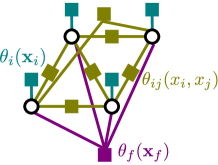
(a) graph structure

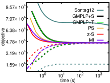
(b) primal and dual

Figure 7: Experiment on synthetic data. (a) Graph structure; (b) Dual objectives (solid line) and the values of decoded integer solution in the primal (dashed line).

GDD based algorithms can be implemented as either a message passing procedure or a belief propagation procedure without messages. We implemented both, and observed that both have similar speed (see Section LABEL:cmp_bp_mp in the supplementary material). Of course, the latter uses less storage. For presentation clarity, we only report the result of GDD using belief propagation without messages here.

7.1 Synthetic data

We generate a synthetic graphical model with a structure commonly used in image segmentation and denoising. The structure is a $128\times 128$ grid shown in Figure 7(a) with 3 types of potentials: node potentials, edge potentials and higher order potentials. We consider the problem below,

$$\max_{\operatorname{\mathbf{x}}}\big{[}\sum_{i\in\operatorname{\mathcal{V}}}\theta_{i}(x_{i})+\sum_{ij\in\operatorname{\mathcal{E}}}\theta_{ij}(x_{i},x_{j})+\sum_{f\in\mathcal{F}}\theta_{f}(\operatorname{\mathbf{x}}_{f})\big{]},$$

where each $x_{i}\in\{1,2,3\}$ and $|f|=4$. All potentials are generated from normal distribution $N(0,1)$. For clusters with order $\geq 4$, Sontag12 only enforces local marginalisation constraints from clusters to nodes, thus its initial local marginal polytope is looser than that of GMPLP and our methods. As shown in Figure 7(b), the proposed methods, converge much faster than GMPLP+S, GMPLP+T and Sontag12. Also Sontag12’s gap between the dual objective and the decoded primal objective is much larger than that of our methods and GMPLP (even with cluster pursuit to tighten the local marginal polytope).

7.2 Protein-Protein Interaction

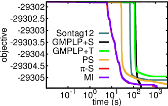
(a) protein2

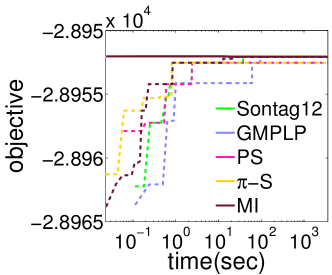
(b) protein4

Figure 8: Dual objectives on 2 PPI problems. (a) On protein2, all algorithms get exact solution except Sontag12, GMPLP+T and PS; (b) On protein4, all algorithms find the exact solution except GMPLP+{T,S}.

Table 2: Average running time ($\pm$ standard deviation) for one iteration of updating all beliefs or messages on PPI dataset

Methods	Average Running Time (sec)
Sontag12	0.0765$\pm$0.0113
GMPLP+S	0.1189$\pm$0.0093
GMPLP+T	0.1118$\pm$0.0020
PS	0.0359$\pm$0.0052
$\pi$-S	0.0120$\pm$0.0030
MI	0.0112$\pm$0.0020

Here we consider 8 Protein-Protein Interaction (PPI) inference problems (from protein1 to protein8) used in Sontag et al (2012). In each problem, there are typically over 14000 nodes, and more than 42000 potentials defined on nodes, edges and triplets. Since the highest order of the potentials is only 3 (triplets), the local marginal polytopes (without cluster pursuit) of all methods here are the same tight. Thus performance difference here is mainly due to different cluster pursuit strategies and computational complexity per iteration.

We test all methods on all 8 problems. The average running time for one iteration of updating all beliefs or messages in Table 2 (i.e. steps 4-7 in Algorithm 2 for ours, and the counterpart for the competitors similar to steps 4-8 in Algorithm 1). We can see that the proposed methods have the smallest average running time, followed by Sontag12, and then by GMPLP.

We present dual objective plots on two problems in Figure 8 here, and provide the results for all problems in the supplementary (Section 8.2). Overall, the proposed methods converge fastest and two of them ($\pi$-S and MI) find exact solutions on 3 problems: protein2, protein4 and protein8. Sontag12 finds exact solutions on protein4 and protein8, and achieved the smallest dual objective values on the problems where all methods failed to find the exact solutions. In terms of convergence, Sontag12 converges slower than proposed methods and faster than GMPLP. GMPLP+T does not find an exact solution on any of the 8 problems, and GMPLP+S finds the exact solution on protein2 only.

7.3 Image Segmentation

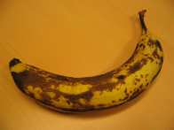
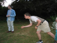
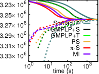
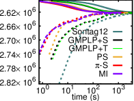
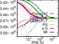
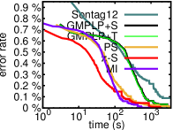
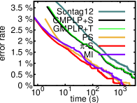
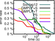
banana1                           bool                             book

Figure 9: Image segmentation results. First row: original images; Second row: segmentations corresponding exact solutions of the MAP inference problems; Third row: decoded primal objectives (dashed line) and dual objectives (solid line); Fourth row: error rate plots. Each column corresponds to the results of one image.

Image segmentation is often seen as a MAP inference problem over PGMs. Following Kohli et al (2009), we consider the MAP problem below

$$\max_{\operatorname{\mathbf{x}}}\big{[}\sum_{i\in\operatorname{\mathcal{V}}}\theta_{i}(x_{i})+\sum_{ij\in\operatorname{\mathcal{E}}}\theta_{ij}(x_{i},x_{j})+\sum_{f\in\mathcal{F}}\theta_{f}(\operatorname{\mathbf{x}}_{f})\big{]}.$$

where $|f|=4$. We use the same graph structure as in Figure 7(a), and follow the potentials in Kohli et al (2009), where the colour terms in $\theta_{i}(x_{i})$ are computed as in Blake et al (2004). More details including parameter settings are provided in the supplementary material. Here we segment three images: banana1, book and bool in the MSRC Grabcut dataset . The resolution of the images varies from $520\times 450$ to $640\times 480$, and each of the inference problems has about $2\times 10^{5}$ to $3\times 10^{5}$ nodes and more than $10^{6}$ potentials. Sontag12 failed to find exact solutions in all 3 images. GMPLP+S and GMPLP+T find exact solution on book only. The proposed methods, PS, $\pi$-S and MI, find the exact solution on all three problems. The result is shown in Figure 9. From the third row of Figure 9 (primal-dual objetives), we can see that the proposed method converges much faster than the competitors. From the fourth row of Figure 9, we can see that the inference error rate (against the exact solution) reduced quickest to zero for the proposed methods.

7.4 Image Matching

Here we consider key point based image matching between two images (a source image and a destination image). First we detect key points from both images via SIFT Lowe (1999) detector. Assume that there are $m$ key points from the source image and $n$ key points from the destination image. Let $\{p(i)\in\mathbb{R}^{2}\}_{i=1,2,\ldots,m}$ and $\{q(i)\in\mathbb{R}^{2}\}_{i=1,2,\ldots,n}$ be the coordinates of key points in the source and the destination images respectively. Let $\{h(i)\}_{i=1,2,\ldots,m}$ and $\{g(i)\}_{i=1,2,\ldots,n}$ be the SIFT feature vectors of the source and the destination images respectively. Assume $m\leq n$ (otherwise swap the source image and the destination image to guarantee so). The task is for each key point $i\in\{1,2,\ldots,m\}$ in the source image, to find a corresponding key point $x_{i}\in\{1,2,\ldots,n\}$ in the destination image. When there are a large number of points involved, a practical way is to restrict a corresponding key point $x_{i}\in\{1,\ldots,k\}\cup\{-1\}$. Here if $i$ has a corresponding point, we restrict it from its $k$-nearest neighbours of the SIFT feature vector $h(i)$ in $\{q(i)\in\mathbb{R}^{2}\}_{i=1,2,\ldots,n}$. If $i$ has no corresponding point, we let $x_{i}=-1$.

Let $\operatorname{\mathcal{V}}=\{1,2,\ldots m\}$, and the matching problem can be formulated as a MAP problem similar to Li et al (2010),

$$\max_{\operatorname{\mathbf{x}}}\Big{\{}\sum_{i\in\operatorname{\mathcal{V}}}\theta_{i}(x_{i})+\sum_{f\in\mathcal{F}}\theta_{f}(\operatorname{\mathbf{x}}_{f})\Big{\}},$$ (82)

where $|f|=4$, $x_{i}\in\{1,\ldots,k\}\cup\{-1\}$, and constructing of $\operatorname{\mathcal{F}}$ is provided in the supplementary. In Li et al (2010), key points in the source image are filtered and reduced to less than 100 (see Section 3 of Li et al (2010)), thus they often have corresponding key points in the destination image. As a result they did not use $-1$ to handle the no correspondence case. However, this strategy gives rise to a danger that potentially important key points may be removed too. Also the small scale of their problem allows them to let $x_{i}$ take all $n$ states. In our experiment, we keep all key points (often over $10^{3}$ in both source and destination images). In that situation, we face two issues: 1) each $f\in\operatorname{\mathcal{F}}$ needs $\operatorname{\mathcal{O}}((k+1)^{4})$ storage for potentials and beliefs; 2) some key points in the source image have no corresponding points in the destination image. For the first issue, we set $k=4$ for computational efficiency. For the second issue, we extend the models in Li et al (2010) to handle the potential lack of correspondence. The node and higher order potentials are defined as follows:

$$\theta_{i}(x_{i}) =\left\{\begin{array}[]{cl}-\eta&x_{i}=-1\\ -\delta_{i}||h(i)-g(x_{i})||_{2}^{2}&\mathrm{otherwise}\end{array}\right.$$

$$\theta_{f}(\operatorname{\mathbf{x}}_{f}) =\left\{\begin{array}[]{cl}0&\exists i\in f,s.t.x_{i}=-1\\ -||P_{\operatorname{\mathbf{x}}_{f}}W_{f}||_{1}&\mathrm{otherwise}\end{array}\right.$$

bikes

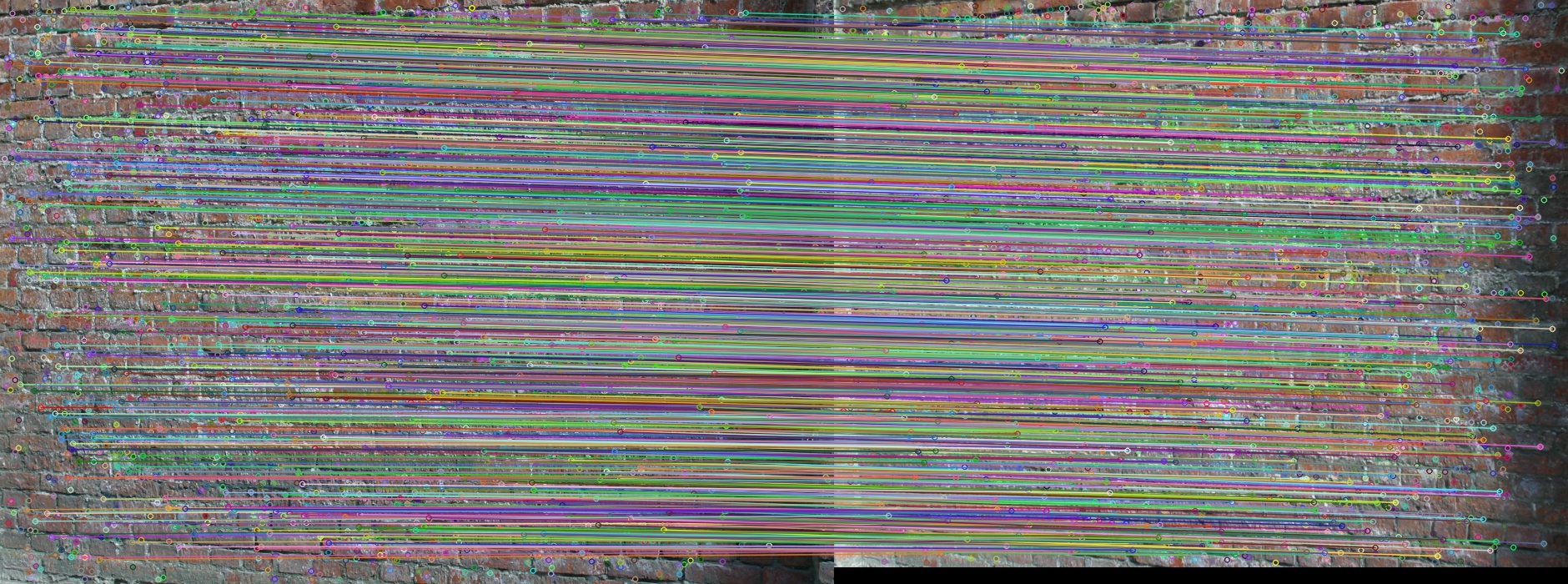
wall

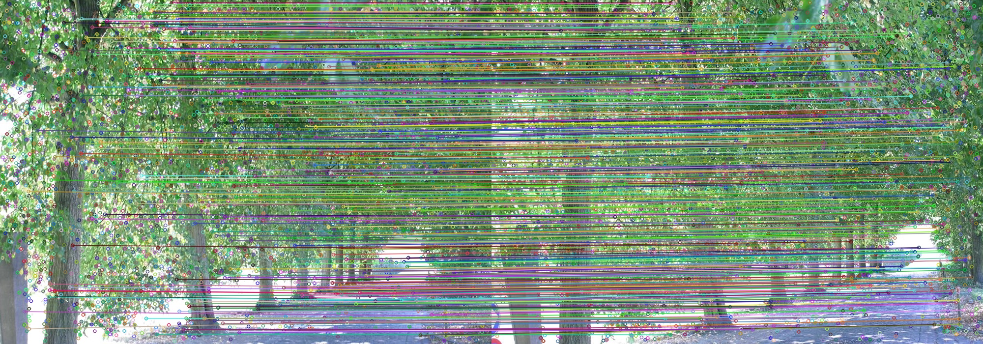
trees

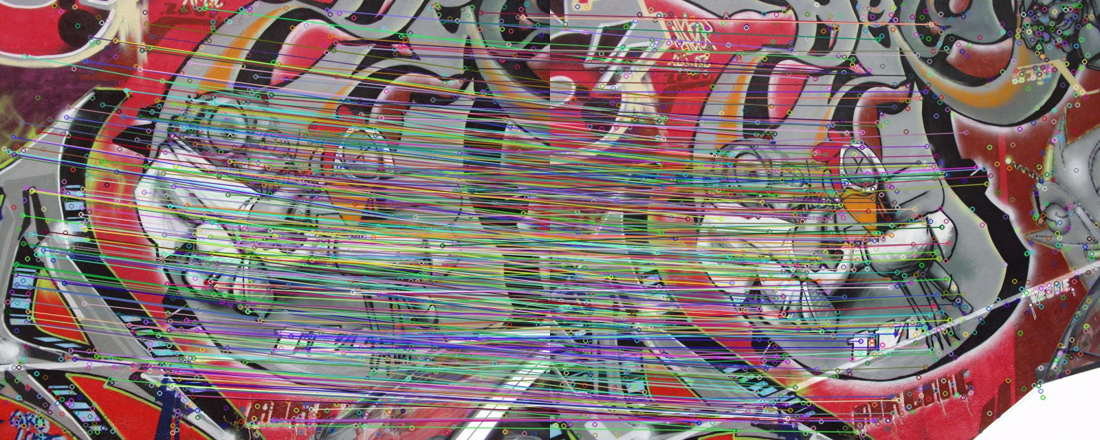
graf

bark

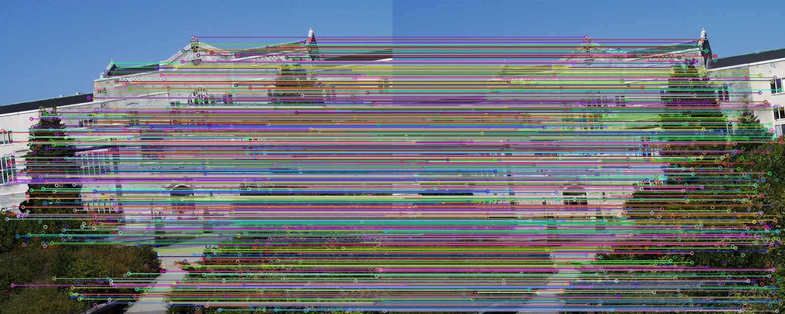
ubc

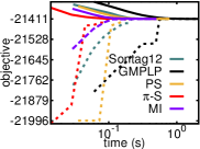
bikes12(1219)

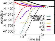
wall12(2184)

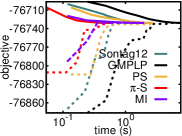
trees12(3284)

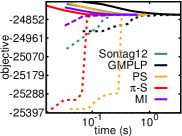
graf12(1203)

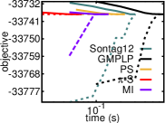
bark12(1486)

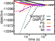
ubc12(1182)

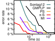
bikes12(1219)

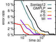
wall12(2184)

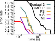
trees12(3284)

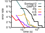
graf12(1203)

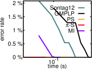
bark12(1486)

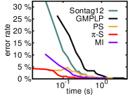
ubc12(1182)

Figure 10: Image matching result. Top 2 rows: images and matching results; Middle 2 rows: decoded primal (dashed line) and dual (solid line); Bottom 2 rows: error rate plots. $[d]ij(n)$ means matching between $i^{th}$ image and $j^{th}$ image in dataset $[d]$, with a PGM of $n$ nodes.

where $\eta$ and $\delta_{i}$ are user specified parameters, $P_{\operatorname{\mathbf{x}}_{f}}=[q(x_{i})]_{i\in f}\in\mathbb{R}^{2\times 4}$, and $W_{f}\in\mathbb{R}^{4}$ is a column vector computed via solving (5) in Li et al (2010) (details provided in supplementary).

We set $\eta=-25$, and $\delta_{i}=100/\max_{x_{i}}||h(i)-g(x_{i})||_{2}^{2},\forall i\in\operatorname{\mathcal{V}}$. We test all algorithms on 6 image sequences from Affine Covariant Regions Datasets . Each inference problem has about $1\times 10^{3}$ to $3\times 10^{3}$ nodes and $2\times 10^{3}$ to $6\times 10^{3}$ potentials. All algorithms find exact solutions. GMPLP converges before using cluster pursuit, thus GMPLP+S and GMPLP+T became the same (reported as GMPLP). From Figure 10 we can see that our $\pi$-S converges fastest among all methods in all images, followed by our MI.

Table 3: Running time comparison. Total running time and the averaged ranking (Avg. Rank) of the speed are reported. Best results are in boldface (the smaller the better).

	bark12	bark23	bark34	bark45	bark56	bikes12	bikes23	bikes34
Sontag12	0.30	1.00	0.38	1.29	0.66	0.70	0.65	0.61
GMPLP	0.68	2.07	2.10	5.35	2.77	2.10	2.44	1.25
PS(Ours)	0.23	1.30	0.33	1.37	0.77	0.79	1.00	0.41
$\pi$-S(Ours)	0.07	0.60	0.13	0.51	0.24	0.18	1.14	0.10
MI(Ours)	0.14	0.78	0.23	0.92	0.44	0.50	0.59	0.25

	bikes45	bikes56	graf12	graf23	graf34	graf45	graf56	trees12
Sontag12	0.30	0.55	0.69	0.54	1.31	2.52	1.20	2.36
GMPLP	2.11	0.76	3.54	3.66	5.51	3.52	3.28	7.71
PS(Ours)	0.59	0.25	0.90	1.27	1.89	1.68	1.19	2.76
$\pi$-S(Ours)	0.26	0.21	0.21	0.17	0.74	0.33	0.25	0.58
MI(Ours)	0.40	0.20	0.62	0.85	1.43	0.91	0.59	1.99

	trees23	trees34	trees45	trees56	ubc12	ubc23	ubc34	ubc45
Sontag12	3.21	0.87	0.18	1.13	1.15	0.77	0.46	0.33
GMPLP	6.95	3.46	0.76	3.88	4.65	4.88	4.33	1.98
PS(Ours)	1.58	1.61	1.41	1.43	2.04	1.96	1.87	0.48
$\pi$-S(Ours)	1.71	0.40	0.41	0.49	1.09	0.59	0.55	0.97
MI(Ours)	1.14	1.28	0.72	1.59	1.28	1.33	1.29	0.30

	ubc56	wall12	wall23	wall34	wall45	wall56	Avg. Rank
Sontag12	0.05	1.38	1.39	1.21	0.97	0.74	2.600
GMPLP	0.19	5.32	7.93	5.68	2.52	2.26	4.933
PS(Ours)	0.11	1.68	3.33	2.05	0.85	1.15	3.567
$\pi$-S(Ours)	0.04	1.49	10.75	1.06	0.95	0.94	1.700
MI(Ours)	0.10	1.17	1.77	1.75	0.52	0.93	2.200

Table 4: Iterations comparison. Number of iterations and the averaged ranking (Avg. Rank) are reported. Best results are in boldface (the smaller the better).

	bark12	bark23	bark34	bark45	bark56	bikes12	bikes23	bikes34
Sontag12	7	24	9	31	18	26	23	23
GMPLP	7	22	23	58	34	34	38	21
PS(Ours)	4	24	6	25	16	22	27	12
$\pi$-S(Ours)	3	28	6	24	13	13	80	7
MI(Ours)	3	17	5	20	11	17	19	8

	bikes45	bikes56	graf12	graf23	graf34	graf45	graf56	trees12
Sontag12	16	41	22	15	33	64	28	21
GMPLP	51	25	51	45	62	40	34	32
PS(Ours)	24	14	22	27	36	33	21	20
$\pi$-S(Ours)	26	30	13	9	35	16	11	10
MI(Ours) 8	19	13	18	21	32	21	12	16

	trees23	trees34	trees45	trees56	ubc12	ubc23	ubc34	ubc45
Sontag12	29	6	1	8	36	23	12	9
GMPLP	29	12	2	12	66	66	52	24
PS(Ours)	11	10	7	8	49	45	38	10
$\pi$-S(Ours)	30	6	5	6	67	34	28	49
MI(Ours)	9	9	4	10	37	36	29	7

	ubc56	wall12	wall23	wall34	wall45	wall56	Avg. Rank
Sontag12	1	20	21	19	15	11	2.600
GMPLP	2	35	54	40	17	15	4.200
PS(Ours)	2	18	37	25	10	13	2.967
$\pi$-S(Ours)	2	44	288	32	27	27	2.867
MI(Ours)	2	16	24	25	7	12	1.833

Both the total running time and the number of iterations required to reach an exact solution for the matching problems are reported in Tables 3 and 4. In several cases $\pi$-S takes an abnormally long time because it was trapped at a local optimum and cluster pursuit had to be applied to escape its basin of attraction. Two of the proposed methods, PS and $\pi$-S, take less running time and iterations in most cases as number of constraints and variables is sufficiently reduced without loosening the local marginal polytope.

8 Conclusion

We have proposed a unified formulation of MAP LP relaxations which allows to conveniently compare different LP relaxation with different formulations of objectives and different dimensions of primal variables. With the unified formulation, a new tool, the Marginal Polytope Diagram, is proposed to describe LP relaxations. With a group of propositions, we can easily find equivalence between different marginal polytope diagrams. Thus constraint reduction can be carried out via the removal of redundant nodes and replacement of equivalent edges in the marginal polytope diagram. Together with the unified formulation and constraint reduction, we have also proposed three new message passing algorithms, two of which have shown significant speed up over the state-of-the-art methods. Extension to marginal inference is of future work.

See pages - of supp.pdf

References

• Batra et al (2011) Batra D, Nowozin S, Kohli P (2011) Tighter relaxations for map-mrf inference: A local primal-dual gap based separation algorithm. In: International Conference on Artificial Intelligence and Statistics, pp 146–154
• Blake et al (2004) Blake A, Rother C, Brown M, Perez P, Torr P (2004) Interactive image segmentation using an adaptive gmmrf model. In: Computer Vision-ECCV 2004, Springer, pp 428–441