Signatures of Coherent Vortex Structures in a Disordered 2D Quantum Fluid

Abstract

The emergence of coherent rotating structures is a phenomenon characteristic of both classical and quantum 2D turbulence. In this work we show theoretically that the coherent vortex structures that emerge in decaying 2D quantum turbulence can approach quasi-classical rigid-body rotation, obeying the Feynman rule of constant average areal vortex density while remaining spatially disordered. By developing a rigorous link between the velocity probability distribution and the quantum kinetic energy spectrum over wavenumber $k$, we show that the coherent vortex structures are associated with a $k^{3}$ power law in the infrared region of the spectrum, and a well-defined spectral peak that is a physical manifestation of the largest structures. We discuss the possibility of realizing coherent structures in Bose–Einstein condensate experiments and present Gross-Pitaevskii simulations showing that this phenomenon, and its associated spectral signatures, can emerge dynamically from feasible initial vortex configurations.

I Introduction

The emergence of coherent rotating structures from disordered flows is a central feature of 2D classical turbulence Kraichnan and Montgomery (1980); Tabeling (2002); Boffetta and Ecke (2012). In two-dimensional quantum turbulence (2DQT) Numasato and Tsubota (2010); Numasato et al. (2010); Bradley and Anderson (2012); Reeves et al. (2012); Neely et al. (2013); Wilson et al. (2013); White et al. (2013a), the analogous phenomenon involves large-scale clustering of quantum vortices of the same sign of circulation; such clustering can occur in negative temperature equilibrium states Onsager (1949); Eyink and Sreenivasan (2006); Billam et al. (2013), and as a result of a turbulent inverse-energy cascade induced by small-scale forcing Reeves et al. (2013). The characterization of such clustered vortex states, which tend to be highly disordered arrangements of same-sign vortices, poses a theoretical challenge of recent interest White et al. (2012); Reeves et al. (2012). In many respects, these states strongly contrast with a rotating superfluid in its ground state, which will form a regular Abrikosov lattice comprised of co-rotating vortices, exhibiting a sixfold rotational symmetry, and obeying Feynman’s rule of constant areal vortex density Feynman (1955); Fetter (2009). Although the velocity field of the superfluid is formally curl-free, the velocity field of a large lattice approaches that of rigid-body rotation under appropriate coarse-graining over many vortex cores Fetter and Svidzinsky (2001), as required by Bohr’s correspondence principle. Furthermore, the self-similar expansion of the atomic density of a 3D turbulent cloud Henn et al. (2009) can be modelled by introducing a rotational velocity field Caracanhas et al. (2012), suggesting that the development of a rotational velocity field in an irrotational superfluid may be a fundamental property of quantum turbulence. In the context of the negative temperature states arising as the end states of decaying 2DQT Billam et al. (2013), these considerations motivate the question: what kind of rotational velocity field emerges in the interior of a large, coherent vortex cluster?

In this work we address the problem of characterizing emergent coherent vortex structures in a 2D Bose-Einstein condensate (BEC), a compressible superfluid, with an emphasis on experimentally accessible measures. While measurements of vortex locations and circulations White et al. (2012); Reeves et al. (2013), or of two-point velocity correlations would allow inference of the classical (point-vortex-like) energy spectrum Bradley and Anderson (2012); Nore et al. (1997), neither the vortex circulations, nor the velocity correlations are easily accessed in current 2DQT experiments Wilson et al. (2013); Neely et al. (2013). These difficulties motivate an exploration of other measures that may be more easily accessible. Here, we consider information contained in the quantum kinetic energy spectrum of the quantum fluid; provided interactions can be suppressed using, for example, an appropriate Feshbach resonance, this information may be readily available in experiments via ballistic expansion Thompson et al. (2014). We develop a link between the quantum kinetic energy spectrum over wavenumber $k$ and the superfluid velocity probability distribution, and show analytically that a spectrum $E(k)\propto k^{3}$ in the infrared arises from the coherent quantum vortex structures emerging in negative-temperature vortex configurations. We show analytically that such a spectrum can correspond to rigid-body rotation, extending to a scale determined by the size of the coherent vortex structures, and, additionally, can arise due to quadrupole velocity fields resulting from the interaction between the coherent structures and the superfluid boundary.

We numerically sample vortex configurations over a range of energies, exploring a number of measures with which to characterize the vortex distributions. We verify the emergence of a $k^{3}$ spectrum and demonstrate that the coherent structures produce a well-defined peak in the quantum kinetic energy spectrum. This peak can be quantitatively understood by considering the largest vortex structures. We further find that the largest structures exhibit a constant areal vortex density, and conclude that the clustered states that emerge in negative-temperature configurations obey Feynman’s rule while being spatially disordered. We consider the outlook for observing quasi-classical coherent vortex structures in atomic BEC experiments. Dynamical simulations of a trapped BEC (within the damped Gross-Pitaevskii description) show that, for well-chosen non-equilibrium vortex configurations that may be accessible via laser-stirring protocols Neely et al. (2010), the resulting vortex dynamics can form long-lived, high-energy coherent vortex structures despite some loss of energy to sound.

Our main result is that quasi-classical coherent structures exhibiting rigid-body rotation can emerge in negative-temperature vortex states, establishing a new link between classical and quantum turbulence that may be explored experimentally.

This paper is structured as follows. In Sec. II we introduce relevant background, and the classical spectral decomposition frequently used in the literature. In Sec. III we develop a decomposition of the quantum kinetic energy spectrum of the quantum fluid, and show its connection to the velocity probability distribution for a compressible superfluid in the hydrodynamic regime. In Sec. IV we present our numerical methods for sampling and analyzing clustered states, and analyze kinetic energy spectra of vortex distributions over a range of energies for vortex configurations in a doubly-periodic box. In Sec. V we analytically and numerically investigate the emergence of quasi-classical flows for negative-temperature states. In Sec. VI we show that high-energy coherent vortex structures, and the associated spectral signatures, can emerge dynamically in a trapped BEC, and compare the properties of the dynamically-generated structures to the properties predicted by microcanonical sampling. Sec. VII presents concluding remarks.

II Background

We consider a BEC that is tightly confined in the $z$-direction. The Gross-Pitaevskii equation describing this homogeneous 2D Bose gas is written in terms of an effective 2D interaction parameter $g_{2}$:

$$i\hbar\frac{\partial\psi({\mathbf{r}},t)}{\partial t} = \left(-\frac{\hbar^{2}\nabla_{\perp}^{2}}{2m}+g_{2}|\psi({\mathbf{r}},t)|^{2}\right)\psi({\mathbf{r}},t),$$ (1)

where $g_{2}=g/l$, $l$ is the characteristic thickness of the 3D system Numasato et al. (2010), and $g=4\pi\hbar^{2}a_{s}/m$ for $s$-wave scattering length $a_{s}$ and atomic mass $m$. For example, in a system with harmonic trapping in the $z$-direction characterized by trapping frequency $\omega_{z}$, the length scale is $l=\sqrt{2\pi}l_{z}$ where $l_{z}=\sqrt{\hbar/m\omega_{z}}$ is the $z$-axis harmonic oscillator length, and the confinement is assumed sufficient to put the wavefunction into the $z$-direction single-particle harmonic oscillator ground state. We note, however, that such tight confinement in one direction is not necessarily required for studies of 2DQT Rooney et al. (2011); Neely et al. (2013).

II.1 Properties of a 2D Quantum Vortex

For solutions with chemical potential $\mu$ containing a single vortex at the origin (with circulation necessarily normal to the plane of the 2D quantum fluid) we can write Fetter and Svidzinsky (2001)

$$\psi_{1}({\mathbf{r}},t)=\sqrt{n_{0}}e^{-i\mu t/\hbar}\chi\!\left(r/\xi\right)e^{\pm i\theta}$$ (2)

where $\xi=\hbar/mc$ is the healing length for speed of sound $c=\sqrt{\mu/m}$, and $n_{0}=\mu/g_{2}$ is the 2D particle density for $r\gg\xi$ and is taken to be a constant. The vortex radial amplitude function $\chi({\sigma})$, where ${\sigma}=r/\xi$ is a scaled radial coordinate, is a solution of

$$\left(-{\sigma}^{-1}\partial_{\sigma}\,{\sigma}\partial_{\sigma}+{\sigma}^{-2}\right)\chi=2(\chi-\chi^{3}).$$ (3)

The boundary conditions are $\chi(0)=0$, and the derivative $\chi^{\prime}\equiv d\chi/d{\sigma}$ evaluated at ${\sigma}=0$ must be chosen such that it is consistent with $\chi(\infty)=1$ and $\chi^{\prime}(\infty)=0$. The value

$$\Lambda\equiv\chi^{\prime}(0)=\lim_{r\to 0}\frac{\xi}{\sqrt{n_{0}}}\left|\frac{d\psi_{1}}{dr}\right|$$ (4)

is a universal feature of the vortex core, and numerically is found to be $\Lambda=0.8249\dots$ Bradley and Anderson (2012). The quantum vortex state (2) has the velocity field of a point-vortex

$$\mathbf{v}({\mathbf{r}})=\frac{\hbar}{mr}(\mp\sin\theta,\pm\cos\theta)=(v_{x},v_{y}),$$ (5)

which has vorticity, $\omega({\mathbf{r}})=\partial_{x}v_{y}-\partial_{y}v_{x}$, given by

$$\omega(\mathbf{r})=\pm\frac{h}{m}\delta(\mathbf{r}),$$ (6)

where $\delta(\mathbf{r})$ is the Dirac $\delta$-function.

II.2 Hydrodynamic decomposition

The 2D Gross-Pitaevskii energy in the homogeneous system is given by

$$\mathcal{E}=\int d^{2}\mathbf{r}\left\{\frac{\hbar^{2}}{2m}|\nabla\psi(\mathbf{r},t)|^{2}+\frac{g_{2}}{2}|\psi(\mathbf{r},t)|^{4}\right\}.$$ (7)

Using the Madelung representation $\psi(\mathbf{r},t)=\sqrt{\rho(\mathbf{r},t)}e^{i\theta(\mathbf{r},t)}$ which gives the superfluid velocity as ${\mathbf{v}}(\mathbf{r},t)=\hbar\nabla\theta(\mathbf{r},t)/m$, the energy can be decomposed as $\mathcal{E}=\mathcal{E}_{H}+\mathcal{E}_{Q}+\mathcal{E}_{I}$, where

$$\mathcal{E}_{H} = \frac{m}{2}\int d^{2}{\mathbf{r}}\;\rho({\mathbf{r}},t)|\mathbf{v}({\mathbf{r}},t)|^{2},$$ (8)

$$\mathcal{E}_{Q} = \frac{\hbar^{2}}{2m}\int d^{2}{\mathbf{r}}\;|\nabla\!\sqrt{\rho({\mathbf{r}},t)}|^{2},$$ (9)

$$\mathcal{E}_{I} = \frac{g_{2}}{2}\int d^{2}{\mathbf{r}}\;\rho({\mathbf{r}},t)^{2}.$$ (10)

Respectively, these define the hydrodynamic kinetic energy, quantum pressure energy, and interaction energy. The hydrodynamic and quantum pressure terms originate from the kinetic energy term, and $\mathcal{E}_{K}=\mathcal{E}_{H}+\mathcal{E}_{Q}$ is the total kinetic energy.

II.3 Classical Kinetic Energy Spectrum

It is worthwhile to briefly review the spectral decomposition often used in the literature, for example Ref. Nore et al. (1997). We call this the classical kinetic energy spectrum, as in a classical fluid it is exactly the kinetic energy power spectrum. This spectrum is obtained by applying the general correspondence between a two-point correlation function and its associated power spectrum to the velocity field. However, as we will show in Sec. III, in a quantum fluid the existence of a quantum phase $\theta(\mathbf{r})$ breaks this correspondence. While in a quantum fluid this classical spectrum is no longer the kinetic energy spectrum, it provides a useful link to classical turbulence theory, allowing the identification of, for example, the Kolmogorov $k^{-5/3}$ law associated with an inertial range.

As we will only focus on particular instants in time, we now drop the explicit time dependence from our notation. By Parseval’s theorem, (8) may be equivalently written in wavenumber $(k)$-space as

$$\mathcal{E}_{H}=\frac{m}{2}\int d^{2}{\mathbf{k}}\;|\tilde{{\mathbf{u}}}({\mathbf{k}})|^{2},$$ (11)

where

$$\tilde{{\mathbf{u}}}({\mathbf{k}})=\mathcal{F}[{\mathbf{u}}(\mathbf{r})]\equiv\frac{1}{2\pi}\int d^{2}{\mathbf{r}}\;e^{-i{\mathbf{k}}\cdot{\mathbf{r}}}\mathbf{u}({\mathbf{r}}),$$ (12)

and ${\mathbf{u}}(\mathbf{r})=\sqrt{\rho(\mathbf{r})}{\mathbf{v}}(\mathbf{r})$ is the density-weighted velocity field. The one-dimensional spectral density in $k$-space is given in polar coordinates by integrating over the azimuthal angle to give

$$\epsilon_{H}(k) = \frac{mk}{2}\int_{0}^{2\pi}d\theta_{k}\;|\tilde{{\mathbf{u}}}({\mathbf{k}})|^{2}$$ (13)

$$= \frac{mk}{2}\int_{0}^{2\pi}d\theta_{k}\;\left|\frac{1}{2\pi}\int d^{2}\mathbf{r}\;e^{-i\mathbf{k}\cdot\mathbf{r}}{\mathbf{u}}(\mathbf{r})\right|^{2}$$ (14)

which, when integrated over all $k$, gives the total hydrodynamic kinetic energy $\mathcal{E}_{H}=\int_{0}^{\infty}dk\;\epsilon_{H}(k)$. Similarly, for the quantum pressure we have

$$\epsilon_{Q}(k)\equiv\frac{\hbar^{2}}{2m}k\int_{0}^{2\pi}d\theta_{k}\left|\frac{1}{2\pi}\int d^{2}\mathbf{r}\;e^{-i\mathbf{k}\cdot\mathbf{r}}\nabla\sqrt{\rho(\mathbf{r})}\right|^{2},$$ (15)

and the total kinetic energy is given by $\mathcal{E}_{K}=\mathcal{E}_{H}+\mathcal{E}_{Q}=\int dk\>[\epsilon_{H}(k)+\epsilon_{Q}(k)]$.

The hydrodynamic spectrum $\epsilon_{H}(k)$ can be further decomposed into incompressible and compressible parts via a Helmholtz decomposition, writing ${\mathbf{u}}={\mathbf{u}}^{i}+{\mathbf{u}}^{c}$, where $\nabla\cdot{\mathbf{u}}^{i}=0$ and $\nabla\times{\mathbf{u}}^{c}=0$. The incompressible part is associated with quantum vortices, whereas the compressible part is associated with acoustic excitations Numasato et al. (2010); Bradley and Anderson (2012). Although we do not make direct use of this decomposition here, we are generally interested in the incompressible limit, where ${\mathbf{u}}\approx{\mathbf{u}}^{i}$. As a single vortex is purely incompressible Bradley and Anderson (2012), the incompressible limit corresponds to a fluid for which the background density is smoothly varying, and the quantum vortices are sufficiently well-separated that their cores do not overlap.

It has become standard in the literature to interpret the incompressible and compressible parts of $\epsilon_{H}(k)$ loosely as kinetic energy densities in $k$-space Reeves et al. (2013); Kobayashi and Tsubota (2005); Numasato et al. (2010), as is the case for classical fluids, and thus these kinetic energy densities are generally referred to as “incompressible” and “compressible” spectra. However, this approach does not provide a true kinetic energy spectrum that can be directly connected to the momentum distribution of a quantum fluid. Furthermore, the classical “spectra” are not locally additive in $k$-space, complicating the identification of energy fluxes.

III Kinetic Energy Spectrum and Velocity Probability Distribution

In this section we pursue an alternative route to decomposing the kinetic energy of the quantum fluid, and develop a link between the true quantum kinetic energy spectrum and the velocity probability distribution.

III.1 Quantum Kinetic Energy Spectrum

The kinetic energy of the quantum fluid is given by

$$\mathcal{E}_{K}=\frac{\hbar^{2}}{2m}\int d^{2}\mathbf{r}\;|\nabla\psi(\mathbf{r})|^{2}.$$ (16)

This may be equivalently written in momentum space as

$$\mathcal{E}_{K}=\frac{\hbar^{2}}{2m}\int d^{2}\mathbf{k}\;|\mathbf{k}\phi(\mathbf{k})|^{2},$$ (17)

where

$$\phi(\mathbf{k})=\frac{1}{2\pi}\int d^{2}\mathbf{r}\;e^{-i\mathbf{k}\cdot\mathbf{r}}\psi(\mathbf{r}).$$ (18)

Writing $\mathbf{k}=k(\cos\theta_{k},\sin\theta_{k})$, and performing the angular integration, we obtain the quantum kinetic energy spectrum

$$E(k)=\frac{\hbar^{2}k^{3}}{2m}\int_{0}^{2\pi}d\theta_{k}\;|\phi(\mathbf{k})|^{2},$$ (19)

and the total kinetic energy via $\mathcal{E}_{K}=\int_{0}^{\infty}dk\;E(k)$.

We now provide a decomposition of the quantum kinetic energy spectrum that allows the identification of hydrodynamic and quantum pressure components, and their relationship to the momentum distribution. Returning to Eq. (17), the integrand can be decomposed using (18) and the Madelung transformation.

We thus write the total kinetic energy as

$$\mathcal{E}_{K} = \int_{0}^{\infty}dk\;E(k)$$ (20)

$$= \int_{0}^{\infty}dk\;\left[E_{H}(k)+E_{Q}(k)+E_{QH}(k)\right],$$ (21)

where

$$E_{H}(k) = \frac{mk}{2}\int_{0}^{2\pi}d\theta_{k}\left|\frac{1}{2\pi}\int d^{2}\mathbf{r}\;e^{-i\mathbf{k}\cdot\mathbf{r}+i\theta(\mathbf{r})}\mathbf{u}(\mathbf{r})\right|^{2},$$ (22)

$$E_{Q}(k) = \frac{\hbar^{2}k}{2m}\int_{0}^{2\pi}d\theta_{k}\left|\frac{1}{2\pi}\int d^{2}\mathbf{r}\;e^{-i\mathbf{k}\cdot\mathbf{r}+i\theta(\mathbf{r})}\nabla\sqrt{\rho(\mathbf{r})}\right|^{2},\;\;\;$$ (23)

$$E_{QH}(k) = \frac{\hbar k}{2}\int_{0}^{2\pi}d\theta_{k}\Phi(\mathbf{k}),$$ (24)

and

$$\Phi(\mathbf{k}) = \frac{-i}{(2\pi)^{2}}\int d^{2}\mathbf{r}e^{-i\mathbf{k}\cdot\mathbf{r}+i\theta(\mathbf{r})}\nabla\sqrt{\rho(\mathbf{r})}$$ (25)

$$\cdot\int d^{2}\mathbf{r}^{\prime}e^{i\mathbf{k}\cdot\mathbf{r}^{\prime}-i\theta(\mathbf{r}^{\prime})}\mathbf{u}(\mathbf{r}^{\prime})$$

$$+\mathrm{c.c.},$$

with $\mathrm{c.c.}$ denoting the complex conjugate. Equations (22), (23), and (24) give the kinetic energy spectra for the hydrodynamic, quantum pressure, and quantum-hydrodynamic components respectively.

The decomposition derived above provides genuine spectral energy densities, as they are locally additive in $k$-space: $E_{H}(k)+E_{Q}(k)+E_{QH}(k)=E(k)$. In contrast, although integrating the classical spectra yields $\mathcal{E}_{H}+\mathcal{E}_{Q}=\mathcal{E}_{K}$, the classical spectra are not locally additive in $k$-space: $\epsilon_{H}(k)+\epsilon_{Q}(k)\neq E(k)$. The hydrodynamic and quantum pressure terms here differ to those of the classical spectral decomposition by the formal replacement $\mathbf{u}(\mathbf{r})\rightarrow e^{i\theta(\mathbf{r})}\mathbf{u}(\mathbf{r})$ from (14) to (22) and $\nabla\sqrt{\rho(\mathbf{r})}\rightarrow e^{i\theta(\mathbf{r})}\nabla\sqrt{\rho(\mathbf{r})}$ from (15) to (23). Notice also that there is no term corresponding to the quantum-hydrodynamic term (24) in the classical kinetic energy decomposition. Furthermore, as

$$\mathcal{E}_{K}=\mathcal{E}_{H}+\mathcal{E}_{Q}=\int_{0}^{\infty}dk\;[\epsilon_{H}(k)+\epsilon_{Q}(k)]\\ =\int_{0}^{\infty}dk\;[E_{H}(k)+E_{Q}(k)+E_{QH}(k)],$$ (26)

we may conclude that

$$\int_{0}^{\infty}dk\;E_{QH}(k)=0,$$ (27)

illustrating that the quantum-hydrodynamic term does not contribute to the total energy, and serves only to redistribute the energy in $k$-space. Another important property of the quantum kinetic energy spectrum [Eq. (19)] is its potential experimental accessibility: The momentum distribution of a non-interacting condensate, $|\phi(\mathbf{k})|^{2}$, can be obtained through ballistic (time-of-flight) expansion Thompson et al. (2014); Dalfovo et al. (1999). Thus, after suppressing interatomic interactions via an appropriate Feshbach resonance, one can obtain $E(k)$ to high accuracy.

The spectral decomposition we have introduced here thus highlights an important distinction between classical and quantum fluids. In a quantum fluid Eq. (22) is the true hydrodynamic kinetic energy spectrum, whereas Eq. (13) is the power spectrum of the velocity autocorrelation function. In a classical fluid there is no quantum phase, and hence there is no distinction between these two measures. We remark that the quantum spectra may resemble the classical spectra in regimes where the phase $\theta(\mathbf{r})$ is approximately constant over large regions of the system, for example in the vortex-dipole gas regime Chesler et al. (2013) (see also Sec. IV).

III.2 Velocity Probability Distribution

The probability, $P(v)$, that an atom has velocity $v=|{\mathbf{v}}|$ is

$$P(v)=\frac{1}{N_{\rm{tot}}}\int d^{2}\mathbf{r}\;\delta(v-|{\mathbf{v}}(\mathbf{r})|)|\psi(\mathbf{r})|^{2},$$ (28)

for $N_{\rm{tot}}=\int d^{2}\mathbf{r}\;|\psi(\mathbf{r})|^{2}$ atoms, where the normalization is $\int_{0}^{\infty}dv\;P(v)=1$. Note that binning the velocity neglects the density weighting, and so in the context of 2DQT is equivalent to the above for a homogenous superfluid with coreless vortices White et al. (2010); Paoletti et al. (2008). The physical distinction is important in regions where the atomic density is rapidly varying, such as near a quantum vortex core.

Let us briefly consider the velocity probability distribution of a single vortex in a homogeneous, compressible superfluid. We start by calculating $P(v)$ for atoms in a superfluid vortex, given by (2), in an otherwise homogeneous 2D system. Using (2), (5), and (28), and exploiting cylindrical symmetry, yields

$$P(v)=\frac{2\pi n_{0}\xi^{2}}{cN_{\rm{tot}}}\left(\frac{c}{v}\right)^{3}\left|\chi\left(\frac{c}{v}\right)\right|^{2}H(v/v_{R}),$$ (29)

where we have introduced the system size $R$, and the Heaviside function $H(v/v_{R})$ restricts the range of velocities to $v\geq v_{R}\equiv c\xi/R=\hbar/mR$, avoiding infrared divergence. Two regimes can be identified within (29), namely a point-vortex regime for $v_{R}\leq v\ll c$ (where $r\gg\xi$ )

$$P(v)\Big{|}_{v\ll c}\simeq\frac{\xi^{2}}{R^{2}}\frac{2}{c}\left(\frac{c}{v}\right)^{3},$$ (30)

and a vortex core regime for $v\gg c$ ($r\ll\xi$)

$$P(v)\Big{|}_{v\gg c}\simeq\frac{\xi^{2}}{R^{2}}\frac{2\Lambda^{2}}{c}\left(\frac{c}{v}\right)^{5}.$$ (31)

Notice the parameter $\Lambda$ [Eq. (4)] appears in the vortex core regime, whereas this is absent in (30). The $v^{-5}$ power law seen here stems from the structure of a vortex core in an atomic Bose-gas superfluid. In a macroscopically occupied BEC with small healing length, the vortex core region only corresponds to a tiny fraction of the atoms. However, it might be possible to observe the $v^{-5}$ power law when the system contains many vortices and few particles, namely, in the vortex-liquid phase Fetter (2009).

The $v^{-3}$ power-law tail of Eq. (30) is a universal result for quantum vortices Paoletti and Lathrop (2011), and has been identified in the 2D and 3D GPE White et al. (2010), the point-vortex model in 2D Min et al. (1996); Weiss et al. (1998), and in superfluid helium Paoletti et al. (2008); Adachi and Tsubota (2011), which is well-described by a vortex-filament model at larger scales. As the $v^{-3}$ power-law is a single vortex effect Paoletti et al. (2008); White et al. (2010); Paoletti and Lathrop (2011)), it will be present in, but is not indicative of, turbulent vortex dynamics. For scales smaller than the minimum inter-vortex distance but appreciably larger than the healing length, the single-vortex velocity field can be expected to dominate the distribution. However, effects due to cooperative behaviour of many quantum vortices are central to quantum turbulence Bradley and Anderson (2012); Billam et al. (2013), and may lead to different behavior for scales greater than the minimum inter-vortex distance Baggaley and Barenghi (2011); Adachi and Tsubota (2011).

III.3 Quantum Kinetic Energy Spectrum in the Hydrodynamic Regime

In this subsection we evaluate the definition of the spectrum (22) within a hydrodynamic approximation that neglects high-order density and phase gradients. This approximation gives a rigorous link between the velocity probability distribution and the quantum kinetic energy spectrum, applicable for a system of quantum vortices in a smoothly varying background density, while neglecting the density variations occurring within distance $\xi$ of a vortex core.

We confine our attention to the hydrodynamic kinetic energy spectrum $E_{H}(k)$. Performing the integral over $\theta_{k}$, the spectrum (22) becomes

$$E_{H}(k) = \frac{mk}{2}\frac{1}{2\pi}\int d^{2}\mathbf{r}\int d^{2}\mathbf{r}^{\prime}e^{i\left[\theta(\mathbf{r})-\theta(\mathbf{r}^{\prime})\right]}$$ (32)

$$\times\sqrt{\rho(\mathbf{r})\rho(\mathbf{r}^{\prime})}{\mathbf{v}}(\mathbf{r})\cdot{\mathbf{v}}(\mathbf{r}^{\prime})J_{0}(k|\mathbf{r}-\mathbf{r}^{\prime}|).$$

Transforming to coordinates $\mathbf{x}=(\mathbf{r}+\mathbf{r}^{\prime})/2$, and $\mathbf{y}=\mathbf{r}-\mathbf{r}^{\prime}$, we Taylor expand in powers of $\mathbf{y}$ to give

$$\theta(\mathbf{x}+\mathbf{y}/2)-\theta(\mathbf{x}-\mathbf{y}/2) \approx \mathbf{y}\cdot\nabla\theta(\mathbf{x})=\frac{m}{\hbar}\mathbf{y}\cdot{\mathbf{v}}(\mathbf{x}),$$ (33)

$$\sqrt{\rho(\mathbf{x}+\mathbf{y}/2)}\sqrt{\rho(\mathbf{x}-\mathbf{y}/2)} \approx \rho(\mathbf{x})-\frac{1}{4}\left(\mathbf{y}\cdot\nabla\sqrt{\rho(\mathbf{x})}\right)^{2},$$ (34)

$${\mathbf{v}}(\mathbf{x}+\mathbf{y}/2)\cdot{\mathbf{v}}(\mathbf{x}-\mathbf{y}/2) \approx |{\mathbf{v}}(\mathbf{x})|^{2}-\frac{1}{4}\left|(\mathbf{y}\cdot\nabla){\mathbf{v}}(\mathbf{x})\right|^{2},$$ (35)

yielding the expression

$$E_{H}(k) \approx \frac{mk}{2}\frac{1}{2\pi}\int d^{2}\mathbf{x}\int d^{2}\mathbf{y}\;e^{im{\mathbf{v}}(\mathbf{x})\cdot\mathbf{y}/\hbar}J_{0}(ky)$$ (38)

$$\times\Bigg{[}\rho(\mathbf{x})|{\mathbf{v}}(\mathbf{x})|^{2}$$

$$-\frac{\rho(\mathbf{x})}{4}\big{|}(\mathbf{y}\cdot\nabla){\mathbf{v}}(\mathbf{x})\big{|}^{2}-\frac{|{\mathbf{v}}(\mathbf{x})|^{2}}{4}\left(\mathbf{y}\cdot\nabla\sqrt{\rho(\mathbf{x})}\right)^{2}$$

$$+\frac{1}{16}\left(\mathbf{y}\cdot\nabla\sqrt{\rho(\mathbf{x})}\right)^{2}\big{|}(\mathbf{y}\cdot\nabla){\mathbf{v}}(\mathbf{x})\big{|}^{2}\Bigg{]}.$$

We may write this as $E_{H}(k)\approx E_{H}^{(0)}(k)+E_{H}^{(2)}(k)+E_{H}^{(4)}(k)$, where the superscripts denote the orders of $\nabla$ involved in each term. In this paper we take a hydrodynamic approach and treat the lowest order term, validating the results against a full numerical treatment. Considering the lowest order term, Eq. (38), and performing the angular integral in $\mathbf{y}$ gives

$${E}_{H}^{(0)}(k) = \frac{mk}{2}\frac{1}{2\pi}\int d^{2}\mathbf{x}\;\rho(\mathbf{x})|{\mathbf{v}}(\mathbf{x})|^{2}$$ (39)

$$\times\int_{0}^{\infty}ydy\;J_{0}\left(\frac{ym|{\mathbf{v}}(\mathbf{x})|}{\hbar}\right)J_{0}(ky).$$

This can be evaluated using the Bessel closure relation $\int_{0}^{\infty}xdx\;J_{\alpha}(ux)J_{\alpha}(vx)=\delta(u-v)/u$, to give the useful result

$$E_{H}^{(0)}(k) = \frac{m}{2}\int d^{2}\mathbf{r}\;\rho(\mathbf{r})|{\mathbf{v}}(\mathbf{r})|^{2}\delta\left(k-\frac{m|{\mathbf{v}}(\mathbf{r})|}{\hbar}\right).$$ (40)

At this level of approximation, the kinetic energy is a simple local transform of the hydrodynamic kinetic energy.

Given the above, let us note that integrating over $k$ gives

$$\int_{0}^{\infty}dk\;E_{H}^{(0)}(k)=\frac{m}{2}\int d^{2}\mathbf{r}\;\rho(\mathbf{r})|{\mathbf{v}}(\mathbf{r})|^{2}\equiv\mathcal{E}_{H},$$ (41)

and our approximations have not affected the total energy. Furthermore, using (28) with (40), we have

$$E_{H}^{(0)}(k)=N_{\rm{tot}}\frac{\hbar}{2}\left(\frac{\hbar k}{m}\right)^{2}P\left(\frac{\hbar k}{m}\right),$$ (42)

where the total hydrodynamic kinetic energy is given by

$$\int_{0}^{\infty}E_{H}^{(0)}(k)dk = N_{\rm{tot}}\int_{0}^{\infty}dv\;P(v)\frac{mv^{2}}{2}.$$ (43)

The expression (42) is our main analytical result, providing a rigorous link between the velocity distribution and the kinetic energy spectrum in the hydrodynamic regime. A superfluid state comprised of quantized vortices in a homogeneous background will be very well described by this expression for the kinetic energy in the regime $k\ll\xi^{-1}$, provided $\mathcal{E}_{H}$ is the dominant energy contribution, and the system does not contain a significant amount of acoustic energy.

Eq. (42) further emphasizes the difference between the classical and quantum kinetic energy spectra in a quantum fluid. The classical spectrum, Eq. (13), contains information about the spatial structure of velocity correlations, but it is not a true kinetic energy spectrum for quantum fluids. Nevertheless, it is the classical spectrum of a quantum fluid which is actually analogous to the kinetic energy spectrum of classical fluids, the incompressible part of which can exhibit, for example, the Kolmogorov scaling Kobayashi and Tsubota (2005); Reeves et al. (2013); Kobyakov et al. (2014), and spectral condensation Billam et al. (2013). In contrast, whilst the quantum kinetic energy spectrum, Eq. (22), draws information from the velocity probability distribution [as shown in Eq. (42)], it has no obvious classical counterpart.

III.4 Spectral Signatures of Coherent Structure Formation

For systems containing many vortices and little compressible energy, the quantum kinetic energy spectrum should be well described by the hydrodynamic approximation Eq. (42). We now consider the spectral features that may be observed for systems containing coherent vortex structures.

A fundamental property of superfluidity is the constraint that the vorticity $\omega(\mathbf{r})=0$ except at vortex cores where it is singular. However, as is well known from the study of Abrikosov vortex lattices, the coarse-grained velocity field can acquire a rotational component as the system approaches a classical state Fetter and Svidzinsky (2001), consistent with Bohr’s correspondence principle. Denoting the classical velocity field by ${\mathbf{v}}_{c}(\mathbf{r})$, the rotational part can be described by the ansatz

$${\mathbf{v}}_{c}(\mathbf{r}) = \mathbf{\Omega}_{c}\times\mathbf{r},$$ (44)

for some $\bm{\Omega}_{c}=\Omega_{c}\hat{\mathbf{z}}$. Ignoring the vortex core structure, the probability distribution for a cluster of radius $R_{c}$ exhibiting rigid-body rotation is found from (28) as

$$P(v) = \frac{n_{0}}{N_{\rm{tot}}}\int d^{2}\mathbf{r}\;\delta(v-\Omega_{c}r)=\frac{2\pi n_{0}}{\Omega_{c}N_{\rm{tot}}}\int_{0}^{R_{c}}rdr\;\delta(r-v/\Omega_{c})$$ (45)

$$= \frac{2\pi n_{0}}{\Omega_{c}^{2}N_{\rm{tot}}}v\;H\left(\frac{\Omega_{c}R_{c}}{v}\right),$$

where the Heaviside function limits this behavior to the cluster interior. This distribution, with (42), gives the power-law form $E_{H}^{(0)}(k)\sim k^{3}$ for $k\leq k_{c}$, where

$$k_{c}=m\Omega_{c}R_{c}/\hbar,$$ (46)

giving a relation between the cluster size, classical vorticity field, and the $k^{3}$ scale range in the spectrum. Note that the $k^{3}$ form is quite distinct from the infrared result for a single vortex, for which (30) and (42), immediately yield $E_{H}^{(0)}(k)\propto k^{-1}$.

For any finite system with a sufficiently high level of clustering, there will be significant modifications to the velocity field due to the interactions between the coherent structures and the boundary (or, equivalently, the image vortices that ensure the flow obeys the boundary conditions). For vortex distributions containing both positive and negative vortices, highly energetic, maximum-entropy configurations take the form of a macroscopic dipole Eyink and Sreenivasan (2006); Billam et al. (2013). The interaction between the clusters that form this dipole with their image vortices will induce a quadrupole mode in the phase, which will generate a stagnation point in the velocity field. The phase in the vicinity of a stagnation point may be modelled as $\theta(\mathbf{r})=\alpha xy$, where $\alpha$ is a constant with dimensions of inverse area Recati et al. (2001) (see Sec.  IV for examples of this phase structure). The velocity field is thus given by

$$\mathbf{v}_{s}=\frac{\hbar\alpha}{m}(y,x),$$ (47)

and from Eq. (28), one finds

$$P(v)=\frac{2\pi n_{0}m^{2}}{\hbar^{2}|\alpha|^{2}N_{\rm tot}}v\;H\left(\frac{R_{s}\hbar|\alpha|}{mv}\right)$$ (48)

with the Heaviside function limiting the behavior to some region $r<R_{s}$. Here $P(v)$ again yields the spectrum $E^{(0)}_{H}(k)\sim k^{3}$. Eqs. (45) and (48) suggest that a significant region of the quantum kinetic energy spectrum may exhibit a $k^{3}$ power law if coherent vortex structures are present in the system. We also note from Eq. (19) that a $k^{3}$ spectrum corresponds to a constant momentum distribution. We explore the quantum kinetic energy spectrum further in the following section, where we examine vortex distributions via numerical sampling.

IV Numerical sampling and spectral analysis of coherent vortex structures

In order to characterize the emergence of coherent vortex structures, we consider the end-states of freely decaying (i.e., unforced) 2DQT. Such states can be sampled using microcanonical methods Billam et al. (2013) and, in the case of appropriate experimental small-scale forcing Reeves et al. (2013), are expected to form via the subsequent freely-evolving vortex dynamics after switching off the forcing mechanism.

Figure 1: (Top row) Vortex distributions for a range of point-vortex energies. The distribution has been decomposed into clusters, dipoles and free vortices using the RCA Reeves et al. (2013) (see text). For $\epsilon\geq 5$, $\mathbf{R}$ and $|\mathbf{r}-\mathbf{R}|=R_{c}$ are shown by crosses and dashed lines respectively. Vortices in clusters are connected by solid lines showing the minimal spanning tree of the cluster. In each panel the field of view is $L\times L$, where $L=512\xi$. (Middle row) Phase profiles $\theta(\mathbf{r})$ for the corresponding vortex distributions. (Bottom row) Log-log graphs of the quantum kinetic energy spectrum $\langle E(k)\rangle$ [ensemble average of Eq. (19)], and the classical hydrodynamic spectrum $\langle\epsilon_{H}(k)\rangle$ [ensemble average of Eq. (13)] for a range of point-vortex energies, averaged over $40$ random walk trajectories at each energy. Shaded regions show $\pm 1$ standard deviations. Lines proportional to $k^{3}$ (green) are shown for comparison. For $\epsilon\geq 5$ the vertical dashed line and shaded regions show $k^{\rm RCA}_{c}$, and $\pm 1$ standard deviation respectively (see text).

IV.1 Microcanonical Sampling

We consider neutral (zero net circulation) vortex configurations within a doubly-periodic box. We consider configurations of varying point-vortex energy per vortex, which correspond to varying degrees of clustering, and directly correspond to Gross-Pitaevskii energies in the incompressible regime Billam et al. (2013). Following Refs. Weiss and McWilliams (1991); Billam et al. (2013), the energy per vortex for a neutral configuration of $N$ point-vortices with charges $\{\kappa_{j}\}=\pm 1$ (circulations $h\kappa_{j}/m$), located at positions $\{\mathbf{r}_{j}\}$ within a square box of side length $L$ is given in terms of the vortex-pair energy

$$h(\mathbf{r})=\sum_{m=-\infty}^{\infty}\ln\left[\frac{\cosh(x-2\pi m)-\cos(y)}{\cosh(2\pi m)}\right]-\frac{x^{2}}{2\pi}$$ (49)

as

$$\epsilon(\{\mathbf{r}_{j}\},\{\kappa_{j}\})=\epsilon_{0}+\frac{1}{N}\sum_{p=1}^{N-1}\sum_{q=p+1}^{N}\kappa_{p}\kappa_{q}\;h\left(\frac{2\pi(\mathbf{r}_{p}-\mathbf{r}_{q})}{L}\right),$$ (50)

where the point-vortex energy is in units of $\Omega_{0}\xi^{2}$, $\Omega_{0}=\pi\hbar^{2}n_{0}/m\xi^{2}$ is the unit of enstrophy in the homogeneous GPE, and $\epsilon_{0}=-0.1170...$ is a constant that shifts the energy axis such that $\epsilon=0$ corresponds to an uncorrelated vortex distribution .

The canonical momenta of the point-vortex system are the vortex coordinates (up to circulation prefactors) and, as a result, if the spatial domain is bounded so is the volume of accessible phase space Onsager (1949). Consequently, in this system at $\epsilon=\epsilon_{\rm{max}}\approx-0.255$ Campbell and O’Neil (1991); Billam et al. (2013) the structure function $W(\epsilon)$ (i.e. the number of available states at a given energy) reaches a maximum and is monotonically decreasing thereafter as $\epsilon\rightarrow\infty$. Hence for $\epsilon>\epsilon_{\rm{max}}$, the temperature $T=W(\partial W/\partial\epsilon)^{-1}$ is formally negative. These negative temperature states are associated with a tendency for like-sign vortices to aggregate, and the emergence of macroscopic vortex clusters in maximal entropy (equilibrium) configurations Eyink and Sreenivasan (2006). Averaging over the microcanonical ensemble at a given energy (provided $N$ is sufficiently large, to ensure ergodicity) characterizes the end states of decaying 2DQT at that energy.

The validity of this statistical description is dependent on the size (relative to the healing length), the point-vortex energy, and the vortex density of the system. In particular, increasing the energy or vortex density, or decreasing the system size, eventually leads to strong coupling between vortex and sound degrees of freedom. Note, however, that making the incompressible velocity everywhere small compared to the sound speed $c$ greatly reduces the strength of this coupling: a regime where the statistical description is valid can always be reached by increasing the system size (or alternatively reducing the vortex number, although this approach will eventually affect the system dynamics). Previous work has confirmed that the statistical approach correctly describes the end states of decaying turbulence in the damped GPE for energies up to $\epsilon=6$ Billam et al. (2013) (in a box of length $512\xi$ for $384$ vortices). In this work we provide further confirmation of the approach for even higher energies in trapped systems (see Sec. VI).

We investigate the equilibrium states over a range of point-vortex energies via a random-walk procedure. We start with an uncorrelated distribution of $N=386$ vortices in a box of length $L=512\xi$. For an uncorrelated distribution the nearest-neighbour correlation functions $c_{B}=\sum_{p=1}^{N}\sum_{q=1}^{B}\kappa_{p}\kappa_{p}^{(q)}/BN$ (where $\kappa_{p}^{(q)}$ is the $q$th nearest neighbour to vortex $p$) are equal to zero White et al. (2012); Reeves et al. (2013); Billam et al. (2013). The vortices undergo a random walk towards a state with a desired point-vortex energy $\epsilon$, specified within a tolerance of $\Delta\epsilon=\pm 0.01$. A minimum inter-vortex separation of $2\pi\xi$ is enforced to ensure the vortex cores are non-overlapping Bradley and Anderson (2012), such that higher order density gradients may be neglected, consistent with the analysis of Sec. III.3. This effective hard vortex core can also be viewed physically as an approximation to the energy barrier associated with the formation of multiply-quantized vortices in Gross–Pitaevskii theory Fetter and Svidzinsky (2001).

Once a configuration with the desired energy is obtained, we find the corresponding Gross-Pitaevskii wavefunction using the constructive approach developed in Ref. Billam et al. (2013). In brief, the modulus of the wavefunction $\sqrt{\rho(\mathbf{r})}$ is constructed as the product of the individual vortex core wavefunctions [the numerical solution to Eq. (3)]  and the phase $\theta(\mathbf{r})$ is constructed from the sum of the phases due to individual vortex dipoles. We work in units of the healing length $\xi$ and the chemical potential $\mu$. The wavefunctions are constructed on a numerical grid with resolution $M=2048^{2}$. We sample within the range of point-vortex energies $\epsilon=[-3,200]$, sampling over 40 random walk trajectories at each value of $\epsilon$.

IV.2 Recursive Cluster Algorithm

To analyse our vortex distributions, we make use of the recursive clustering algorithm (RCA) presented in Reeves et al. (2013). The algorithm yields detailed spatial information about a particular vortex configuration by decomposing it into clusters, dipoles and free vortices. From the decomposition of the vortex distribution, we may acquire characteristic information about each cluster. In particular, the physical location of the cluster is estimated by the center of mass

$$\mathbf{R}=\frac{1}{N_{c}}\sum_{j\in C}\mathbf{r}_{j}$$ (51)

where $C$ denotes the set of all vortices that belong to a particular cluster, and $N_{c}\equiv|\kappa_{c}|$ denotes the number of vortices in the cluster. Additionally, the spatial extent of a cluster can be estimated by the cluster radius, which we define as the mean distance from the center of mass

$$R_{c}=\frac{1}{N_{c}}\sum_{j\in C}|\mathbf{r}_{j}-\mathbf{R}|.$$ (52)

Although the cluster algorithm yields values for $\mathbf{R}$ and $R_{c}$ for every cluster in a given distribution, throughout this section we are primarily concerned with the largest clusters in the system. Hereafter we will use the above notation to refer to the position and radius of the largest cluster only.

We show the resulting decomposition of the vortex distribution for a range of point-vortex energies in the top row of Fig. 1. Qualitatively, the algorithm captures the well-known physics of the point-vortex model: at negative point-vortex energy, the distribution takes the form of a dipole gas, with many or all vortices being bound in vortex-antivortex pairs. As the point-vortex energy is increased, clusters of same-sign vortices emerge, accumulating more vortices with increasing energy. With further increase of the point-vortex energy, clusters continue to accumulate vortices, but also contract spatially, storing more energy internally rather than accumulating more vortices from the remaining vortex field (as the latter would lower the entropy). At sufficiently high energy ($\epsilon\sim 200$) the phenomenon of supercondensation occurs Kraichnan and Montgomery (1980), and the distribution collapses into two macroscopic clusters, each of charge $N/2$. While such a state is unlikely to be achievable in atomic BEC, the supercondensed state nonetheless demonstrates the limiting physics at very high energy.

IV.3 Spectral Analysis

In the bottom row of Fig. 1 we show the (ensemble-averaged) quantum kinetic energy spectrum $\langle E(k)\rangle$ [Eq. (21)] over a range of point-vortex energies. It is evident that, for positive energies, the spectrum acquires a $k^{3}$ scaling in the infrared. The scaling begins at low $k$ and progresses towards larger wavenumbers as the point-vortex energy of the system is increased. The behavior of the spectrum is in stark contrast with the classical spectrum [Eq. (13)], for which the emergence of large-scale structure is signified by a spectral “pile-up” at length scales of order the system size, as is shown in Fig. 1. Notice however that the two spectra are very similar in the low energy vortex-dipole regime. Even for the relatively modest point-vortex energy $\epsilon=5$ the spectrum exhibits nearly a decade of $k^{3}$ scaling in this system. For sufficiently high energy ($\epsilon\approx 100$) the range of the $k^{3}$ scaling extends past the point $k=\xi^{-1}$. In dynamical simulations, it is unlikely that the $k^{3}$ scaling would extend this far, as effects due to compressibility are non-negligible at velocities comparable to $c$ (see Sec. VI). At high energy, the regions of slowly-varying phase that contribute to the infrared spectrum are clearly seen at the stagnation points and in the interior regions of the largest clusters. In the supercondensed state, the stagnation point phase structure $\theta(\mathbf{r})=\alpha xy$ becomes particularly evident.

Figure 2: Wavenumber corresponding to the peak of the spectrum $k_{c}$, as a function of the point-vortex energy per vortex $\epsilon$. The shaded region and errorbars show $\pm$ 1 standard deviations.

The location of the peak in the kinetic energy spectrum, which we label $k_{c}$, gives an indication of the $k^{3}$ scale-range observed in the negative-temperature regime. In light of Eq. (42), in the hydrodynamic approximation where $v=\hbar k/m$, this wavenumber indicates a most probable or “characteristic” velocity. This characteristic velocity is associated with the coherent structures; as the energy is increased and large structures emerge, we observe that phase fluctuations of a characteristic wavelength develop around these structures, and throughout the system [Fig. 1]. The characteristic wavelength of the fluctuations shortens as $\epsilon$ increases. These observations are consistent with Onsager’s prediction – that the velocity field of a negative-temperature equilibrium state will be dominated by the coherent motion of the macroscopic vortex clusters, since the motion of the remaining vortices is essentially random Eyink and Sreenivasan (2006).

We find that the characteristic velocity can be estimated from the RCA by considering only the largest cluster (in terms of charge) in a given configuration. The wavelength of the phase variations at a distance $r$ from a large cluster will be $\lambda=2\pi r/\kappa_{\rm{net}}$, where $\kappa_{\rm net}$ denotes the net charge within the region enclosed by a circle of radius $r$. The corresponding wavenumber is thus $k=\kappa_{\rm{net}}/r$.

To calculate a value for $k_{c}$ from the RCA data, which we denote $k_{c}^{\rm RCA}$, we take the largest cluster and calculate the net charge enclosed within the cluster’s radius $R_{c}$. We only consider energies at which we may unambiguously define the largest cluster ($\epsilon\geq 5$ ); for these values, $k^{\rm RCA}_{c}$ is shown in Fig. 1 (bottom row), where it clearly provides a good indication of the location of the spectral peak. Conversely, the location of the peak provides a good estimator of the scale of the largest cluster in the system. We also compare $k_{c}$ as calculated directly from the kinetic energy spectrum to $k_{c}^{\rm RCA}$ in Fig. 2. In general there is very good agreement in the data, even though the RCA does not account for cluster anisotropy [e.g. see Fig. 1, $\epsilon=50$]. Agreement is poorest at lower energies ($\epsilon\lesssim 10$), when the largest clusters are not significantly larger than those in the background vortex distribution. However, as the energy is increased, agreement improves as the largest clusters begin to dominate the velocity field.

V Emergence of rigid-body rotation

Figure 3: Azimuthal velocity field $v_{\Omega}$ of the largest cluster, as a function of distance from the cluster center $|\mathbf{r}-\mathbf{R}|$, for a range of point-vortex energies $\epsilon$. Shaded regions show $\pm 1$ standard deviations. Solid (red) lines show a linear fit to the averaged velocity field within the region $0\leq|\mathbf{r}-\mathbf{R}|\leq 40\xi$. The slope yields a value for $\Omega_{c}^{\rm fit}$ (see text and Fig.4). Horizontal and vertical dashed lines show the values $v_{c}^{\rm RCA}/c\equiv k_{c}^{\rm RCA}\xi$ (see Fig. 2) and $\langle R_{c}\rangle$ respectively.

V.1 Azimuthal velocity field

According to the analysis in Sec. III.4, the presence of a $k^{3}$ spectrum suggests that the azimuthal velocity field in the vicinity of a large cluster may mimic that of a rigid body, that is $v_{\theta}(\mathbf{r}^{\prime})=\Omega_{c}|\mathbf{r}^{\prime}|$, where $|\mathbf{r}^{\prime}|=|\mathbf{r}-\mathbf{R}|$ is the distance from the cluster center. However, we have shown that the $k^{3}$ spectrum may also be due to the stagnation points of the velocity field. Due to the non-local nature of the Fourier transform, it is difficult to disentangle the spectral contributions from rigid-body rotation and the stagnation points. This motivates us to analyse the clusters directly, to determine the extent to which they exhibit rigid-body characteristics.

Again considering energies $\epsilon\geq 5$, we calculate the angular velocity field relative to the cluster center, averaging over the azimuthal direction and the ensemble:

$$v_{\Omega}(r^{\prime})=\left\langle{\frac{1}{2\pi}\int_{0}^{2\pi}\;d\theta^{\prime}\;|v_{\theta}(\mathbf{r}^{\prime})|}\right\rangle.$$ (53)

The resulting velocity field for a range of point-vortex energies is shown in Fig. 3. The averaged velocity field is approximately linear over the cluster interior, although fluctuations are larger at lower energy. The linear behaviour is typically maintained up to scales comparable to the average cluster radius $\langle R_{c}\rangle$. At $\langle R_{c}\rangle$ the velocity is well approximated by the characteristic velocity $v_{c}^{\rm RCA}\equiv\hbar k_{c}^{\rm RCA}/m$. We find $v_{\Omega}$ to be linear for at least $r^{\prime}\lesssim 40\xi$ for $\epsilon\geq 5$, and that the slope of $v_{\Omega}$ steepens with increasing $\epsilon$. Note that although the RCA sometimes over estimates the region of linear behavior, the velocity is always well described by $v_{c}^{\rm RCA}$ at $\langle R_{c}\rangle$. Additionally, notice $v_{\Omega}(0)\approx 0$, suggesting that the RCA accurately determines the location of the cluster center.

V.2 Measures of classical vorticity

To further characterize the rigid-body flow field, we may determine the rigid-body rotation frequency $\Omega_{c}$, thus also determining the characteristic turnover time $T=2\pi/\Omega_{c}$ for the largest cluster. We describe four measures:

$\Omega_{c}^{\rm{fit}}$: A value may be obtained from the slope of a linear fit to $v_{\Omega}$. We fit over the region $0\leq r^{\prime}\leq 40\xi$, where linearity holds for all $\epsilon$, as shown by the lines of best fit in Fig. 3. We show $\Omega_{c}^{\rm{fit}}$ as a function of $\epsilon$ in Fig. 4(a). There is a clear linear trend in the data, which are well described by the relation $\Omega_{c}^{\rm{fit}}=(1.5\epsilon+36)\times 10^{-4}$. We use $\Omega_{c}^{\rm fit}$ as a base measure, which we compare against other measures.

$\Omega_{c}^{\rm{Feyn}}$: The positive-temperature ground state for a system rotating at frequency $\Omega_{c}$ is an ordered vortex lattice that has a constant vortex density given by Feynman’s rule, $n_{v}=m\Omega_{c}/\pi\hbar$ Feynman (1955). In order to maintain rigid-body rotation, the negative-temperature clustered states considered in this work must still exhibit a constant area per vortex on average, even though they do not maintain crystalline order. Applying Feynman’s argument, we expect a rotation frequency

$$\Omega_{c}^{\rm Feyn}=\frac{\pi\hbar\langle n_{v}\rangle}{m},$$ (54)

where $\langle n_{v}\rangle$ denotes the average vortex density of the largest cluster in each sample, averaged over the ensemble. Considering the cumulative distribution $N_{v}(r)$, which counts the number of vortices with $|\mathbf{r}_{i}-\mathbf{R}|\leq r$, we find the distribution is well described by $N_{v}(r)=\pi n_{v}r^{2}$ (as required for constant $n_{v}$) over the region where $v_{\Omega}$ is linear. We verify that this is not an artifact of the vortex-separation minimum by reducing the separation cutoff used in our microcanonical sampling from $2\pi\xi$ to $\xi$, finding nearly identical results. Fitting over the same region $0\leq r^{\prime}\leq 40\xi$ yields values for $\Omega_{c}^{\rm Feyn}$ which are in excellent agreement with $\Omega_{c}^{\rm fit}$, as shown in Fig. 4(b). We emphasize that $\Omega_{c}^{\rm fit}$ is obtained from the velocity field, while $\Omega_{c}^{\rm Feyn}$ is determined by the vortex distribution.

$\Omega_{c}^{\rm{RCA}}$: A value for $\Omega_{c}$ may also be calculated from the RCA data. Since the rigid-body velocity field persists up to the characteristic wavenumber $k_{c}=m\Omega_{c}R_{c}/\hbar$, and $k_{c}$ is well described by $k_{c}^{\rm{RCA}}=\kappa_{\rm{net}}/R_{c}$, clearly we may consider

$$\Omega_{c}^{\rm{RCA}}\equiv\left\langle\frac{\hbar\kappa_{\rm{net}}}{mR_{c}^{2}}\right\rangle=\frac{1}{2}\left\langle\frac{1}{\pi R_{c}^{2}}\int_{\mathcal{R}}d^{2}\mathbf{r}\;\omega(\mathbf{r})\right\rangle,$$ (55)

where $\mathcal{R}$ is the region enclosed by a circle of radius $R_{c}$ centered on $\mathbf{R}$. This is equivalent to averaging the vorticity distribution over the region of the cluster. The values $\Omega_{c}^{\rm{RCA}}$ are shown in Fig. 4(c). There is reasonable quantitative agreement between the data obtained directly from the wavefunction ($\Omega_{c}^{\rm fit}$) and that extracted from the RCA. It is clear that there is some discrepancy in qualitative trend however, and agreement between the two quantities is poorest for $\epsilon\sim 120$. This “sag” at intermediate energies is due to a decline in vortex density in the outer region of the cluster, which causes $N_{v}(r)$ to deviate from the expected quadratic behavior, and consequently $v_{\Omega}$ to deviate from rigid-body behavior (Fig. 3, $\epsilon=100$). For perfect rigid body rotation extending out to $R_{c}$, one would expect $\Omega_{c}^{\rm fit}$ and $\Omega_{c}^{\rm RCA}$ to yield exactly the same values. Thus $\Omega_{c}^{\rm RCA}$ indicates the extent to which the velocity field deviates from perfect rigid-body rotation over the scale of the cluster as defined by the RCA value $R_{c}$.

Figure 4: Measures of the rigid-body rotation frequency $\Omega_{c}$. The shaded regions ($\Omega_{c}^{\rm fit}$) and error bars (other measures) indicate $\pm 1$ standard deviations. In (b)-(d) $\Omega_{c}^{\rm fit}$ is shown for comparison.

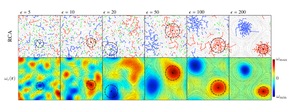
Figure 5: The emergence of classical flows: Exemplar RCA vortex distributions and coarse grained vorticity fields $\omega_{c}(\mathbf{r})$ [the latter obtained by including only spatial modes $k\leq k_{\rm{cut}}=2\pi/(2R_{c})$] for a range of $\epsilon$. Streamlines show the velocity field ${\mathbf{v}}(\mathbf{r})=\hbar\nabla\theta(\mathbf{r})/m$. Crosses show the center-of-mass position of the largest cluster in each sample, $\mathbf{R}$, as determine by the RCA. The RCA radius $R_{c}$ is shown by the dashed line.

$\Omega_{c}^{\rm{class}}$: The presence of a rigid-body velocity field requires that, under an appropriate coarse graining procedure (see also, e.g., Baggaley et al. (2012a, b)), the formally singular vorticity field becomes constant over the central region of the cluster, i.e., $\omega(\mathbf{r})=h/m\sum_{i}\delta(\mathbf{r}-\mathbf{r}_{i})\rightarrow\omega_{c}(\mathbf{r})\simeq 2\Omega_{c}$ for $|\mathbf{r}-\mathbf{R}|\lesssim R_{c}$. Defining an average over many quantum vortices, we consider the coarse-grained classical vorticity field

$$\omega_{c}(\mathbf{r})\equiv\frac{1}{2\pi}\int_{\mathcal{K}}d^{2}\mathbf{k}\;\tilde{\omega}(\mathbf{k})e^{i\mathbf{k}\cdot\mathbf{r}}$$ (56)

where $\tilde{\omega}(\mathbf{k})=\mathcal{F}[\omega(\mathbf{r})]$ and $\mathcal{K}$ is the $k$-space domain satisfying $|\mathbf{k}|<k_{\rm{cut}}=2\pi/\ell_{\rm cut}$ for a chosen cutoff length-scale $\ell_{\rm{cut}}\gg\xi$. Coarse graining over the spatial extent of the largest vortex cluster ($\ell_{\rm{cut}}=2R_{c}$) yields a value consistent with the other measures if we consider $\omega_{c}(\mathbf{r})$ at the cluster center:

$$\Omega_{c}^{\rm{class}}=\left\langle\frac{1}{2}\omega_{c}(\mathbf{R})\right\rangle.$$ (57)

Values for $\Omega_{c}^{\rm class}$ are shown in Fig. 4(d). We find excellent agreement between $\Omega_{c}^{\rm{class}}$ and $\Omega_{c}^{\rm{fit}}$ until $\epsilon\sim 150$, at which point $\Omega_{c}^{\rm{class}}$ deviates to higher values. This discrepancy is due to taking the value locally at $\mathbf{R}$, where the vorticity can be slightly more concentrated, particularly for large clusters, whereas $\Omega_{c}^{\rm{fit}}$ incorporates information away from the cluster center. $\Omega_{c}^{\rm class}$ indicates that, apart from at very high energy, the clusters do not deviate significantly from rigid-body motion in their interior.

Coarse graining over $\ell_{\rm cut}=2\bar{d}$ for mean nearest-neighbour distance $\bar{d}$ (typically $\bar{d}\simeq R_{c}/3$) yields similar values for $\Omega_{c}^{\rm class}$, but with larger fluctuations. For this value of $\ell_{\rm cut}$ we also verify that $\omega_{c}(\mathbf{r}^{\prime})\approx\rm{const.}$ for $|\mathbf{r}^{\prime}|\lesssim R_{c}$. Averaging over the azimuthal direction and ensemble to obtain $\omega_{c}(r^{\prime})$, we find $\langle\omega_{c}(40\xi)\rangle\gtrsim 0.9\langle\omega_{c}(0)\rangle$ at all energies, consistent with the linear $v_{\Omega}$ and quadratic $N_{v}$ observed up to this scale. At the cluster radius, $\langle\omega_{c}(R_{c})\rangle/\langle\omega_{c}(0)\rangle$ $\sim 0.6-0.8$ for low ($\epsilon\lesssim 50$), and high ($\epsilon\gtrsim 150$) energies respectively, and $\langle\omega_{c}(R_{c})\rangle/\langle\omega_{c}(0)\rangle\sim 0.5$ for intermediate energies. This is consistent with the deviation from rigid-body behavior at larger scales as seen in Fig. 3, and as indicated by the qualitative trend of $\Omega_{c}^{\rm RCA}$.

The emergence of a classical flow field from the quantum vortex distribution is qualitatively captured in Fig. 5, where we present particular examples of the vortex distribution (as decomposed by the RCA) and the classical vorticity field $\omega_{c}(\mathbf{r})$ (for $\ell_{\rm cut}=2R_{c}$), generated at various $\epsilon$. As large clusters emerge, they generate macroscopic regions of approximately uniform vorticity, capturing the qualitative features of the emergent quasi-classical velocity field, as shown by the velocity streamlines.

It is interesting to compare the rigid-body rotation property observed here to the rotational properties of coherent structures in classical fluids. The states we have considered here are the freely-decayed states of a turbulent superfluid. Decaying turbulence described by the inviscid Euler equations has been shown to approach the statistical equilibrium predicted by the mean-field Montgomery-Joyce (sinh-Poisson) equation Montgomery et al. (1992); Montgomery and Joyce (1974). With quantum vortices we would expect to recover this regime in the limit $N\rightarrow\infty$. Indeed, the rigid-body rotation observed here in quantum vortex clusters for large $N$ is qualitatively consistent with the form of the doubly-periodic vortex dipole solution of the Montgomery-Joyce equation Pasmanter (1994).

VI Dynamical Emergence in a Trapped System

Finally, we demonstrate that coherent structures and the associated $k^{3}$ power law can emerge dynamically in a trapped system, and compare the dynamical results against sampling. The model we use to describe the dynamics of a 2D Bose gas is the damped Gross-Pitaevskii equation (dGPE):

$$i\hbar\frac{\partial\psi({\mathbf{r}},t)}{\partial t}=(1-i\gamma)(\mathcal{L}-\mu)\psi({\mathbf{r}},t),$$ (58)

where

$$\mathcal{L}=\left(-\frac{\hbar^{2}\nabla_{\perp}^{2}}{2m}+V_{\rm{ext}}(\mathbf{r})+g_{2}|\psi({\mathbf{r}},t)|^{2}\right),$$ (59)

for an external confining potential $V_{\rm ext}(\mathbf{r})$. The damping parameter $\gamma$ describes the finite-temperature effects due to collisions between the condensate and a stationary thermal reservoir with chemical potential $\mu$. Within the framework of $c$-field theory, the dGPE can be obtained from the stochastic projected Gross-Pitaevskii equation for a large BEC in the low-temperature regime, for which the thermal noise is negligible Blakie et al. (2008). The dGPE has been used extensively in quantum turbulence studies Kobayashi and Tsubota (2005); Neely et al. (2010); Numasato and Tsubota (2010); Reeves et al. (2012); Neely et al. (2013), and has been demonstrated to give qualitative agreement with experiment even for relatively high temperatures Neely et al. (2010). We set $\gamma=10^{-5}$, an experimentally realistic value under the conditions for which the dGPE theory is valid Bradley and Anderson (2012). For such a value of $\gamma$, the modifications to the vortex dynamics Törnkvist and Schröder (1997) are essentially negligible over the integration time we consider. The primary effect of the damping is thus to suppress compressible excitations at very high $k$, which are numerically demanding to resolve, yet have little physical effect on the vortex dynamics in the regime of interest here.

We simulate a 2D BEC confined within a circular well or “bucket” potential of radius $R$, i.e.,

$$V_{\rm ext}(\mathbf{r})=V_{0}\{1+\tanh[(r-R)/a]\},$$ (60)

and set $V_{0}/\mu=10$, $R/\xi=200$, and $a/\xi=3$, such that $V_{\rm ext}$ approximates a hard-wall potential. We remark that Bose condensation in a quasi-uniform cylinder has been recently demonstrated experimentally Gaunt et al. (2013).

In this system, the energy of an $N$-vortex configuration may be characterized by the energy per vortex for point-vortices (in units of $\Omega_{0}\xi^{2}$) within a circular domain $D$ of radius $R$ Yatsuyanagi et al. (2005):

$$\epsilon_{\circ}(\{\mathbf{r}_{j}\},\{\kappa_{j}\})=\tilde{\epsilon}-\frac{1}{N}\sum_{p=1}^{N}\sum_{q\neq p}^{N}\kappa_{p}\kappa_{q}\ln\left|\frac{\mathbf{r}_{p}-\mathbf{r}_{q}}{\xi}\right|\\ -\frac{1}{N}\sum_{p=1}^{N}\sum_{q=1}^{N}\kappa_{p}\bar{\kappa}_{q}\ln\left|\frac{\mathbf{r}_{p}-\bar{\mathbf{r}}_{q}}{\xi}\right|,$$ (61)

where $\bar{\mathbf{r}}_{j}=R^{2}\mathbf{r}_{j}/|\mathbf{r}_{j}|^{2}$ is the location of an image vortex with charge $\bar{\kappa}_{j}=-\kappa_{j}$ and $\tilde{\epsilon}\approx-4.158$ shifts the axis such that $\epsilon_{\circ}=0$ corresponds to an uncorrelated distribution, as does $\epsilon_{0}$ in Eq. (50). The images ensure that the velocity field satisfies the boundary condition ${\mathbf{v}}\cdot\hat{\mathbf{n}}\;|_{\partial D}=0$, i.e., that the flow perpendicular to the boundary $\partial D$ is zero everywhere on $\partial D$.

We set the vortex number to $N=112$. Whilst fewer vortices will inevitably lead to larger statistical fluctuations, a lower vortex density is beneficial here as it reduces the radiative loss of vortex energy into the sound field. Reducing the vortex density ensures that the incompressible velocity field is everywhere small compared to the speed of sound $c$, and also lowers the chance of vortex core overlap, thus ensuring that the vortices remain sufficiently well separated such that their Gross–Pitaevskii dynamics are well-approximated by a point-vortex description Fetter (1966).

Figure 6: Time-averaged quantum kinetic energy spectra (left) and vortex distributions (right) for the dynamical system at $t_{i}=0\hbar/\mu$ (top row) and $t_{f}=11300\hbar/\mu$ (middle row). The spectra for the dynamical system are averaged from $t$ to $t+500\hbar/\mu$. The spectrum and distribution at $t_{f}$ can be compared against those of the statistical ensemble (40 samples) at the same point-vortex energy (bottom row). On the spectrum plots, lines proportional to $k^{3}$ are shown for comparison, shaded regions show $\pm 1$ standard deviation, the vertical dashed line shows $k_{c}$ as calculated from the ensemble using Eq. 46, with the shaded vertical band showing $\pm 1$ standard deviation. Symbols for the vortex distribution plots are as denoted in Fig.1

The initial condition, $\psi_{\circ}(\mathbf{r},0)$, is generated via a similar method to that outlined in Sec. IV:

$$\psi_{\circ}(\mathbf{r})=\psi_{\rm TF}(\mathbf{r})e^{i\theta_{\circ}(\mathbf{r})}\prod_{j=1}^{N}\chi(|\mathbf{r}-\mathbf{r}_{j}|/\xi).$$ (62)

Here the Thomas-Fermi wavefunction $\psi_{\rm TF}(\mathbf{r})=\sqrt{(\mu-V_{\rm ext}({\mathbf{r}}))/g_{2}}$ for $V_{\rm ext}({\mathbf{r}})\leq\mu$ and $0$ otherwise, $\chi(r)$ is the radial core profile of an individual quantum vortex [the numerical solution to Eq. (3)], and

$$\theta_{\circ}(\mathbf{r})=\sum_{j=1}^{N}\kappa_{j}\theta_{j}(\mathbf{r})+\bar{\kappa}_{j}{\theta}_{j}(\bar{\mathbf{r}}),$$ (63)

where $\theta_{j}(\mathbf{r})$ is the phase due to an individual positive vortex at $\mathbf{r}_{j}$. We prepare a high-energy [$\epsilon_{\circ}(t_{i})=10.1$], non-equilibrium initial vortex configuration, as shown in Fig 6. The wavefunction is constructed on a spatial domain of length $L=512\xi$, and is discretized on a grid of $M=1024^{2}$. We numerically integrate the dGPE pseudo-spectrally, using an adaptive 4th-5th order Runge-Kutta method Press et al. (2007); Dennis et al. (2013), and a relative error tolerance of $\tau=10^{-5}$. We have confirmed that all statistical measures of the vortex dynamics remain the same for $L=700$, $M=2048$, $\tau=10^{-6}$.

Full dynamical evolution of the condensate density and phase, RCA vortex distribution, and quantum kinetic energy spectrum are provided in the supplemental material Not . The initial configuration is highly unstable, and the horizontal lines of like-charge clusters undergo a roll-up, due to the Kelvin-Helmholtz instability. The initial kinetic energy spectrum, shown in Fig. 6, does not follow the $k^{3}$ power law, but does exhibit a well-defined peak. The peak is due to the initial clustering in the configuration, which produces phase fluctuations of a characteristic wavelength $\lambda\sim 10\xi-20\xi$ Not .

Full relaxation to equilibrium is slow, requiring an integration time of order $10^{4}\hbar/\mu$. However, clear signs of a $k^{3}$ power law emerge after $t\sim 3000\hbar/\mu$, as, at this stage of the evolution, large, quasi-equilibrium clusters have already formed Not . This is consistent with the observations in Ref. Billam et al. (2013), where it is shown that the macroscopic clusters begin to form well before the equilibration time. After $t_{f}=11300\hbar/\mu$ of evolution, the system has clearly reached the equilibrium state containing coherent vortex structures, as shown in Fig 6. Although during the evolution some of the vortex energy is lost to sound, most of the vortex energy is retained [$\epsilon_{\circ}(t_{f})\sim 7.8$], and thus the configuration is still well within the negative temperature regime. It may be that radiative energy loss of the vortex distribution as a whole is partially inhibited by vortex “cross-talk”, a mechanism via which vortices of the same sign can efficiently impart energy to each other through radiation and absorption of sound Parker et al. (2012).

We emphasize that the final energy per vortex $\epsilon_{\circ}=7.8$ is substantial, being analogous to a point-vortex energy in the periodic system considered in Sec. IV of $\epsilon\gg 7.8$. Indeed, using the supercondensation energy ($\epsilon_{\circ}\approx 70$) as a reference, one can consider the final point-vortex energy in the simulation, $\epsilon_{\circ}(t_{f})=7.8$, to be roughly equivalent (interpreted as a fraction of the supercondensation energy) to $\epsilon\approx 22$ in the doubly-periodic system considered in Sec. IV (where supercondensation occurs at $\epsilon\approx 200$). A more quantitative estimate of equivalence can be obtained using the nearest neighbour clustering measure $c_{1}$ (as defined in Sec. IV.1); we find the equilibrium values to be approximately the same ($c_{1}=0.35$) for $\epsilon_{\circ}=7.8$ and $\epsilon\approx 25$, supporting the above analysis.

The quantum kinetic energy spectrum and vortex distribution at $t_{f}$ can be compared against the same quantities obtained from a statistical ensemble, as shown in Fig. 6. The spectra are qualitatively very similar, and nearly identical in the $k^{3}$ region. The RCA value for $k_{c}$ still gives a reasonable indication of the range of $k^{3}$ behaviour and the location of the spectral peak. The vortex distribution as determined by the RCA is also very similar [see Fig. 6].

We propose that the most direct way initial conditions similar to those shown in Fig. 6 could be created is by carefully-controlled laser stirring and manipulation protocols: The field of two-dimensional quantum turbulence has seen several numerical studies of the injection of clustered vortices via optical stirring potentials in recent years White et al. (2012, 2013b); Reeves et al. (2012); White et al. (2013a); Wilson et al. (2013); Stagg et al. (2014), and injection of small vortex clusters has indeed already been demonstrated experimentally Neely et al. (2010). While neutral systems having similar spatial extent (relative to the healing length) and containing as many vortices as we have considered here may be challenging to achieve, they are nonetheless within the scope of current experimental technology.

VII Conclusion

In this work we have shown that the coherent vortex structures that emerge in decaying 2DQT can exhibit quasi-classical rigid-body rotation, obeying the Feynman rule of constant areal vortex density while remaining spatially disordered. By developing a rigorous link between the velocity probability distribution and the quantum kinetic energy spectrum we have shown that these coherent structures are associated with a $k^{3}$ power-law in the infrared region of the spectrum. The power-law region terminates at a peak located the inverse spatial scale of the largest cluster. The $k^{3}$ spectrum and associated peak provide signatures of coherent structure formation that may be measured independently of the vortex configuration data, and should be accessible in atomic BEC experiments. Furthermore, our analysis illuminates the important distinction between the quantum kinetic energy spectrum and the power spectrum of the velocity autocorrelation function in a quantum fluid.

Although individual vortex cores can be observed, charge-sensitive vortex detection remains a significant challenge in atomic BEC experiments. By identifying a clear spectral signature that may be accessible in ballistic expansion imaging, our work paves the way for experimental observations of negative-temperature coherent vortex structures in two-dimensional atomic Bose-Einstein condensates. Experimental confirmation of the Feynman rule at negative temperature may provide further indication of the appearance of rigid-body rotation and the universality of rotational velocity fields in quantum turbulence.

References

- Kraichnan and Montgomery (1980) R. H. Kraichnan and D. Montgomery, “Two-Dimensional Turbulence,” Rep. Prog. Phys. 43, 547 (1980).
- Tabeling (2002) P. Tabeling, “Two-dimensional turbulence: a physicist approach,” Physics Reports 362, 1 (2002).
- Boffetta and Ecke (2012) G. Boffetta and R. E. Ecke, “Two-Dimensional Turbulence,” Annual Review of Fluid Mechanics 44, 427 (2012).
- Numasato and Tsubota (2010) R. Numasato and M. Tsubota, “Possibility of Inverse Energy Cascade in Two-Dimensional Quantum Turbulence,” J. Low Temp. Phys. 158, 415–421 (2010).
- Numasato et al. (2010) R. Numasato, M. Tsubota, and V. S. L’vov, “Direct Energy Cascade in Two-Dimensional Compressible Quantum Turbulence,” Phys. Rev. A 81, 063630 (2010).
- Bradley and Anderson (2012) A. S. Bradley and B. P. Anderson, “Energy Spectra of Vortex Distributions in Two-Dimensional Quantum Turbulence,” Phys. Rev. X 2, 041001 (2012).
- Reeves et al. (2012) M. T. Reeves, B. P. Anderson, and A. S. Bradley, “Classical and quantum regimes of two-dimensional turbulence in trapped Bose-Einstein condensates,” Phys. Rev. A 86, 053621 (2012).
- Neely et al. (2013) T. W. Neely, A. S. Bradley, E. C. Samson, S. J. Rooney, E. M. Wright, K. J. H. Law, R. Carretero-González, P. G. Kevrekidis, M. J. Davis, and B. P. Anderson, “Characteristics of Two-Dimensional Quantum Turbulence in a Compressible Superfluid,” Phys. Rev. Lett. 111, 235301 (2013).
- Wilson et al. (2013) K. E. Wilson, E. C. Samson, Z. L. Newman, T. W. Neely, and B. P. Anderson, “Experimental methods for generating two-dimensional quantum turbulence in Bose–-Einstein condensates,” Annual Review of Cold Atoms and Molecules 1, 261 (2013).
- White et al. (2013a) A. C. White, B. P. Anderson, and V. S. Bagnato, “Vortices and turbulence in trapped atomic condensates,” (2013a), arXiv:1304.5332 .
- Onsager (1949) L. Onsager, “Statistical hydrodynamics,” Nuovo Cimento Suppl. 6, 279 (1949).
- Eyink and Sreenivasan (2006) G. L. Eyink and K. R. Sreenivasan, “Onsager and the Theory of Hydrodynamic Turbulence,” Rev. Mod. Phys. 78, 87 (2006).
- Billam et al. (2013) T. P. Billam, M. T. Reeves, B. P. Anderson, and A. S. Bradley, “Onsager–Kraichnan Condensation in Decaying Two-Dimensional Quantum Turbulence,” (2013), arXiv:1307.6374 .
- Reeves et al. (2013) M. T. Reeves, T. P. Billam, B. P. Anderson, and A. S. Bradley, “Inverse energy cascade in forced two-dimensional quantum turbulence,” Phys. Rev. Lett. 110, 104501 (2013).
- White et al. (2012) A. White, C. Barenghi, and N. Proukakis, “Creation and Characterization of Vortex Clusters in Atomic Bose-Einstein Condensates,” Phys. Rev. A 86, 013635 (2012).
- Feynman (1955) R. P. Feynman, “Application of Quantum Mechanics to Liquid Helium,” Prog. Low Temp. Phys. 1, 17 (1955).
- Fetter (2009) A. L. Fetter, “Rotating trapped Bose-Einstein condensates,” Rev. Mod. Phys. 81, 647 (2009).
- Fetter and Svidzinsky (2001) A. L. Fetter and A. A. Svidzinsky, “Vortices in a Trapped Dilute Bose-Einstein Condensate,” J. Phys. B 13, R135 (2001).
- Henn et al. (2009) E. A. L. Henn, J. A. Seman, G. Roati, K. M. F. Magalhaes, and V. S. Bagnato, “Emergence of Turbulence in an Oscillating Bose-Einstein Condensate,” Phys. Rev. Lett. 103, 045301 (2009).
- Caracanhas et al. (2012) M. Caracanhas, A.L. Fetter, S.R. Muniz, K.M.F. Magalhães, G. Roati, G. Bagnato, and V.S. Bagnato, “Self-similar Expansion of the Density Profile in a Turbulent Bose-Einstein Condensate,” J. Low Temp. Phys. 166, 49 (2012).
- Nore et al. (1997) C. Nore, M. Abid, and M. E. Brachet, “Kolmogorov Turbulence in Low-Temperature Superflows,” Phys. Rev. Lett. 78, 3896 (1997).
- Thompson et al. (2014) K. J. Thompson, G. G. Bagnato, G. D. Telles, M. A. Caracanhas, F. E. A. dos Santos, and V. S. Bagnato, “Evidence of power law behavior in the momentum distribution of a turbulent trapped Bose–Einstein condensate,” Laser Physics Letters 11, 015501 (2014).
- Neely et al. (2010) T. W. Neely, E. C. Samson, A. S. Bradley, M. J. Davis, and B. P. Anderson, “Observation of Vortex Dipoles in an Oblate Bose-Einstein Condensate,” Phys. Rev. Lett. 104, 160401 (2010).
- Rooney et al. (2011) S. J. Rooney, P. B. Blakie, B. P. Anderson, and A. S. Bradley, “Suppression of Kelvon-Induced Decay of Quantized Vortices in Oblate Bose-Einstein Condensates,” Phys. Rev. A 84, 023637 (2011).
- Kobayashi and Tsubota (2005) M. Kobayashi and M. Tsubota, “Kolmogorov Spectrum of Superfluid Turbulence: Numerical Analysis of the Gross-Pitaevskii Equation with a Small-Scale Dissipation,” Phys. Rev. Lett. 94, 065302 (2005).
- Dalfovo et al. (1999) F. Dalfovo, S. Giorgini, L. P. Pitaevskii, and S. Stringari, “Theory of Bose-Einstein Condensation in Trapped Gases,” Rev. Mod. Phys. 71, 463 (1999).
- Chesler et al. (2013) P. M. Chesler, H. Liu, and A. Adams, “Holographic vortex liquids and superfluid turbulence,” Science 341, 368 (2013).
- White et al. (2010) A. C. White, C. F. Barenghi, N. P. Proukakis, A. J. Youd, and D. H. Wacks, “Nonclassical Velocity Statistics in a Turbulent Atomic Bose-Einstein Condensate,” Phys. Rev. Lett. 104, 075301 (2010).
- Paoletti et al. (2008) M. S. Paoletti, M. E. Fisher, K. R. Sreenivasan, and D. P. Lathrop, “Velocity Statistics Distinguish Quantum Turbulence from Classical Turbulence,” Phys. Rev. Lett. 101, 154501 (2008).
- Paoletti and Lathrop (2011) M. S. Paoletti and D. P. Lathrop, “Quantum Turbulence,” Annual Review of Condensed Matter Physics 2, 213 (2011).
- Min et al. (1996) I. A. Min, I. Mezić, and A. Leonard, “Lévy stable distributions for velocity and velocity difference in systems of vortex elements,” Phys. of Fluids 8, 1169 (1996).
- Weiss et al. (1998) J. B. Weiss, A. Provenzale, and J. C. McWilliams, “Lagrangian dynamics in high-dimensional point-vortex systems,” Phys. Fluids 10, 1929 (1998).
- Adachi and Tsubota (2011) H. Adachi and M. Tsubota, “Numerical study of velocity statistics in steady counterflow quantum turbulence,” Phys. Rev. B 83, 132503 (2011).
- Baggaley and Barenghi (2011) A. W. Baggaley and C. F. Barenghi, “Quantum turbulent velocity statistics and quasiclassical limit,” Phys. Rev. E 84, 067301 (2011).
- Kobyakov et al. (2014) D. Kobyakov, A. Bezett, E. Lundh, M. Marklund, and V. Bychkov, “Turbulence in binary Bose-Einstein condensates generated by highly nonlinear Rayleigh-Taylor and Kelvin-Helmholtz instabilities,” Phys. Rev. A 89, 013631 (2014).
- Recati et al. (2001) A. Recati, F. Zambelli, and S. Stringari, “Overcritical Rotation of a Trapped Bose-Einstein Condensate,” Phys. Rev. Lett. 86, 377 (2001).
- Weiss and McWilliams (1991) J. B. Weiss and J. C. McWilliams, “Nonergodicity of point vortices,” Physics of Fluids A: Fluid Dynamics 3, 835 (1991).
- Note (1) This shifting of the energy axis is in fact equivalent to using the alternative expression for the point-vortex energy derived in Campbell and O’Neil (1991), although we use Eq. (50) for our computations as it is more convenient to work with numerically.
- Campbell and O’Neil (1991) L. J. Campbell and K. O’Neil, “Statistics of two-dimensional point vortices and high-energy vortex states,” Journal of Statistical Physics 65, 495 (1991).
- Note (2) We analyze energies for which there is a unique for at least of the random walk trajectories. In the few cases where multiple clusters satisfy , one of these clusters is selected at random.
- Baggaley et al. (2012a) A. W. Baggaley, J. Laurie, and C. F. Barenghi, “Vortex-Density Fluctuations, Energy Spectra, and Vortical Regions in Superfluid Turbulence,” Phys. Rev. Lett. 109, 205304 (2012a).
- Baggaley et al. (2012b) A. W. Baggaley, C. F. Barenghi, A. Shukurov, and Y. A. Sergeev, “Coherent vortex structures in quantum turbulence,” Europhys. Lett. 98, 26002 (2012b).
- Montgomery et al. (1992) D. Montgomery, W. H. Matthaeus, W. T. Stribling, D. Martinez, and S. Oughton, “Relaxation in two dimensions and the “sinh-Poisson” equation,” Phys. Fluids A 4, 3 (1992).
- Montgomery and Joyce (1974) D. Montgomery and G. Joyce, “Statistical Mechanics of “Negative Temperature” States,” Phys. Fluids 17, 1139 (1974).
- Pasmanter (1994) R. A. Pasmanter, “On long-lived vortices in 2-D viscous flows, most probable states of inviscid 2-D flows and a soliton equation,” Phys. Fluids 6, 1236 (1994).
- Blakie et al. (2008) P. B. Blakie, A. S. Bradley, M. J. Davis, R. J. Ballagh, and C. W. Gardiner, “Dynamics and Statistical Mechanics of Ultra-Cold Bose Gases using C-Field Techniques,” Adv. in Phys. 57, 363–455 (2008).
- Törnkvist and Schröder (1997) O. Törnkvist and E. Schröder, “Vortex Dynamics in Dissipative Systems,” Phys. Rev. Lett. 78, 1908 (1997).
- Gaunt et al. (2013) A. L. Gaunt, T. F. Schmid, I. Gotlibovych, R. P. Smith, and Z. Hadzibabic, “Bose-Einstein Condensation of Atoms in a Uniform Potential,” Phys. Rev. Lett. 110, 200406 (2013).
- Yatsuyanagi et al. (2005) Y. Yatsuyanagi, Y. Kiwamoto, H. Tomita, M. M. Sano, T. Yoshida, and T. Ebisuzaki, “Dynamics of Two-Sign Point Vortices in Positive and Negative Temperature States,” Phys. Rev. Lett. 94, 054502 (2005).
- Fetter (1966) A. L. Fetter, “Vortices in an Imperfect Bose Gas. IV. Translational Velocity,” Phys. Rev. 151, 100 (1966).
- Press et al. (2007) W. H. Press, S. A. Teukolsky, W. T. Vetterling, and B. P. Flannery, Numerical Recipes 3rd Edition: The Art of Scientific Computing (Cambridge University Press, 2007).
- Dennis et al. (2013) G. R. Dennis, J. J. Hope, and M. T. Johnsson, “XMDS2: Fast, scalable simulation of coupled stochastic partial differential equations,” Comp. Phys. Comm. 184, 201 (2013).
- (53) See Supplemental Material at [url].
- Parker et al. (2012) N. G. Parker, A. J. Allen, C. F. Barenghi, and N. P. Proukakis, “Coherent cross talk and parametric driving of matter-wave vortices,” Phys. Rev. A 86, 013631 (2012).
- White et al. (2013b) A. C. White, N. P. Proukakis, and C. F. Barenghi, “Topological stirring of two-dimensional atomic Bose-Einstein condensates,” (2013b), arXiv:1303.0640 .
- Stagg et al. (2014) G. W. Stagg, N. G. Parker, and C. F. Barenghi, “Quantum Analogs of Classical Wakes in Bose-Einstein Condensates,” (2014), arXiv:1401.4041 .