Introduction

If a sky survey is to be performed with the VLA, displacing highly competitive PI-led science for a few thousand hours, it will need to facilitate a wide range of scientific goals and have lasting value for many years. The VLA has 3 options: go as wide as possible (e.g. NVSS; Condon et al. 1998), as deep as possible (e.g. Owen & Morrison 2008), or somewhere in the middle (e.g. FIRST, the VLA Galactic plane survey, or Stripe 82; Becker et al. 1995; Stil et al. 2006; Hodge et al. 2011).

If the VLASS adopts a medium/wide-field approach, it will face significant competition from 3 key facilities in the near future. These are the Apertif focal-plane upgrade on the Westerbork Synthesis Radio Telescope (WSRT; Oosterloo et al. 2009), and the MeerKAT (Booth et al. 2009) and ASKAP (Johnston et al. 2008) SKA-pathfinders.

To avoid overlap with these upcoming facilities, this white paper explores parameter space for a deep field where the VLA can capitalize on its key strengths of sensitivity and angular resolution to provide the astronomical community with a unique survey.

Identifying unique parameter space for a VLA sky survey

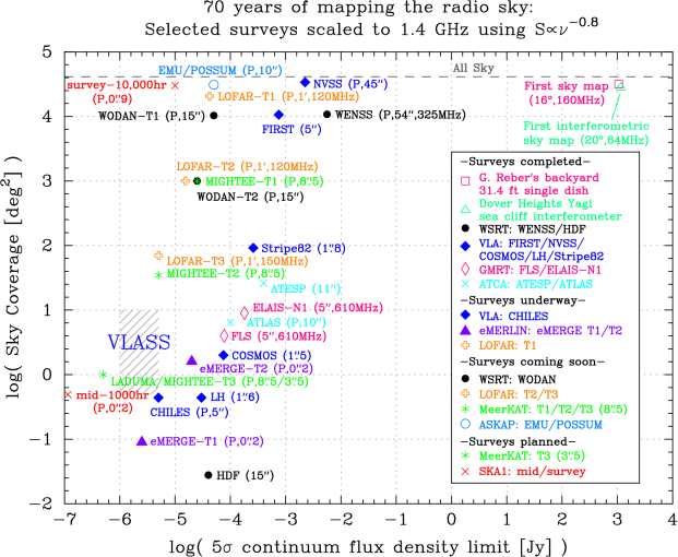
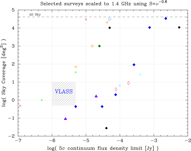
Fig. 1 displays a sample of existing, upcoming, planned, and future surveys with various telescopes. It is clear that within a few years, WSRT, MeerKAT, and ASKAP will have begun and perhaps completed all-sky surveys at L-band in full polarization with angular resolution $>8^{\prime\prime}$, good sensitivity to extended structures, and well-suited to the study of radio transients. Instead of performing a medium/wide-field survey of its own,the VLA may be better suited to targeted follow-up of interesting sources utilizing flexible observing modes.

There is, however, a region of parameter space in Fig. 1 (shaded) that will not be explored until the SKA-era, and which is well-suited for a VLASS: a deep-field survey covering a few square degrees with arcsecond resolution at L-band. Science goals that can be pursued with such a deep-field VLASS are presented later in this white paper.

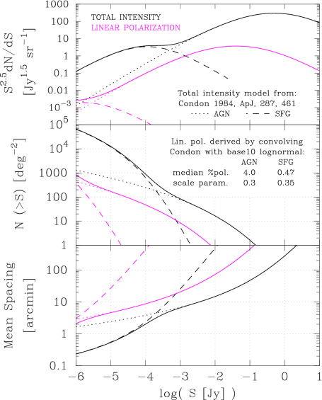
As with FIRST and NVSS, the optimal VLA frequency band to maximize the sky density of extragalactic sources is L-band. This band is also particularly attractive for HI and polarization science (both key drivers for SKA-pathfinder telescopes and the SKA itself), and because the VLA can achieve $<2^{\prime\prime}$ angular resolution in A-configuration (this point is expanded on below). This white paper therefore adopts L-band as optimal. For reference, Fig. 3 presents estimated source counts in total intensity and linear polarization for the L-band extragalactic sky.

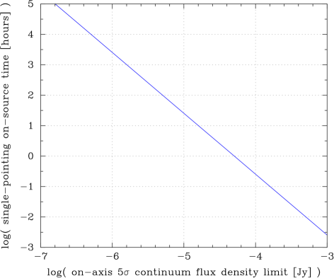
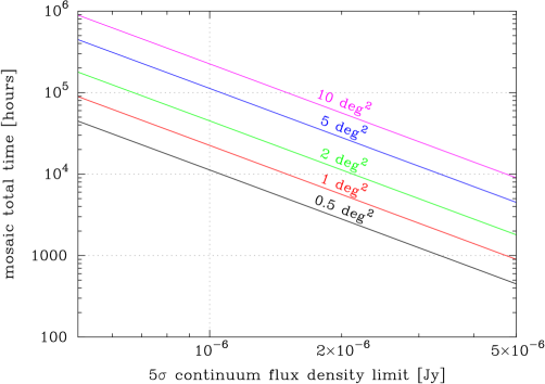
The boundaries for the shaded parameter space in Fig. 1 are selected as follows. The $5\sigma$ flux density upper boundary is set to 5 $\mu$Jy in order to probe deeper than the COSMOS HI Large Extragalactic Survey (CHILES; recently started taking data with the VLA), and to ideally obtain more than a few polarized starburst galaxies per square degree (see top panel of Fig. 3). The survey area upper boundary is set to 10 deg² to keep the total time request below 10,000 hours for a $5\sigma$ flux density upper bound of 5 $\mu$Jy. For reference, Fig. 4 and Fig. 5 present time estimates to reach various $5\sigma$ flux density detection thresholds for a range of survey sizes. The $5\sigma$ flux density lower boundary is set to 1 $\mu$Jy to ensure that a survey area lower boundary of 0.5 deg² can be observed within a total time request of 10,000 hours. Survey areas $<0.5$ deg² can be observed within a single pointing at L-band, though areas $>1$ deg² are likely be preferred for a deep VLASS to minimize influence from cosmic or sample variance.

A-configuration is likely optimal for a deep VLASS for the following reasons. First, arcsecond angular resolution is required for morphological studies of faint radio galaxies (Muxlow et al. 2005); VLA A-configuration may be better suited for such studies than the MeerKAT LADUMA/MIGHTEE tier-3 survey with $3\mbox{$.\!\!^{\prime\prime}$}5$ resolution. Second, the effects of radio interference at L-band are minimized in A-configuration, where the antennas are as far apart as possible. Third, for a given total observing time, the percentage of time lost from PI-led science to a VLASS in A-configuration will be less than for any other configuration (particularly hybrids). Fourth, if a deepA-configuration VLASS is performed over a target field with eMERLIN-eMERGE data (field selection is discussed later in this white paper), then the two surveys can be combined to provide sensitivity to angular scales from $40^{\prime\prime}-0\mbox{$.\!\!^{\prime\prime}$}2$. Only data obtained with VLA’s A-configuration is suitable for combination with eMERLIN data, because the largest angular scale to which eMERLIN is sensitive at L-band is $2^{\prime\prime}$. Finally, confusion is not expected to be an issue in A-configuration at the flux densities considered in this white paper (Condon et al. 2012). Confusion will be an issue for any MeerKAT surveys deeper than MIGHTEE tier-2 until the longest baselines are extended from 8 to 20 km.

Choice of target field

If a deep option is selected for a VLASS, it will be critical to perform the survey over a field with extensive multiwavelength data in order to maximize scientific impact. Community involvement will be required to identify which of the existing multiwavelength extragalactic survey fields is best suited to a heavy investment of VLA time. Some points to consider:

• GOODS-N (12:36+62), XMM-LSS (2:25-5), COSMOS (10:00+2), the Lockman Hole (10:53+57), and the Groth Strip (14:17+52) are the most intensively observed fields in the Northern sky.

• The community may be interested in choosing a field visible to Southern facilities such as the Cerro Chajnantor Atacama Telescope (CCAT) and the Atacama Large Millimeter Array (ALMA), for example.

• Of the four 10 deg² deep drilling fields identified by the Large Synoptic Survey Telescope (LSST) Science Council, two are suitable for a deep VLA survey in A-configuration: XMM-LSS and COSMOS. The former is also one of the Dark Energy Survey (DES) deep supernova survey fields.

• MeerKAT-MIGHTEE tier-2 will target the XMM-LSS and COSMOS fields. This may present an opportunity to combine MeerKAT and VLA data to increase sensitivity to extended structures.

• MeerKAT LADUMA/MIGHTEE tier-3 will target the CDF-S (3:32-28), while eMERLIN-eMERGE tier-1 will target the HDF-N. A deep VLASS on a different field will bring the number of deep fields to three, enabling more robust scientific conclusions to be drawn in the lead-up to the SKA than if only one or two fields were observed.

• The VLA-CHILES survey is currently imaging a single pointing at L-band in B-configuration to a continuum sensitivity of 0.7 $\mu$Jy in the COSMOS field; if a deep VLASS is pursued in the same field, the CHILES data can be included.

Deep field science at L-band

A brief selection of science topics that can be addressed with a deep L-band survey in A-configuration is presented below. While a number of these topics will also be addressed within the next few years by facilities such as WSRT, MeerKAT, and ASKAP, many demand the greater spatial resolving power of the VLA. As a result, a deep L-band VLASS will be of lasting value to the astronomical community well into the SKA-era.

• Faint radio galaxy populations; morphologies, spectral indices, and environments

• Evolution of supermassive black holes, active galaxies (particularly low power), and star formation across cosmic time; luminosity functions

• Strong gravitational lenses, high redshift radio galaxies

• Much like the VLA-CHILES survey, the flexible WIDAR correlator could be set up for a deep VLASS to provide fine spectral resolution over certain redshift rangesfor HI absorption science, and possibly HI emission and recombination line science

• Dark energy and dark matter using radio weak lensing (Blain 2002; Morales 2006; Brown & Battye 2011a, b); high spatial resolution radio polarization and HI data will be very valuable

• The evolution of magnetism in galaxies and large scale structure using radio polarization data (e.g. Akahori et al. 2013); commensal P-band observations could be obtained with L-band, providing improved resolution in Faraday space

• Transient and variable sources

• Degenerate and non-degenerate radio stars

• Develop a gold standard multiwavelength catalog for machine learning algorithms to catalog much wider-area and shallower surveys; for example, SKA1-survey

Figure 1: Comparison of selected radio sky surveys, scaled to 1.4 GHz assuming a spectral index of -0.8. Different telescopes are coded by symbol/color as indicated by the legend. The legend also indicates which surveys are completed, ongoing, coming soon, or planned for future telescopes. The terms in parentheses specify if a polarization catalog was produced (P), the angular resolution, and the observing frequency if not at 1.4 GHz. For a given amount of telescope time, a survey must trade sensitivity with sky coverage; deep and wide surveys (upper left corner) are the most expensive. A simplified version of this figure is presented in Fig. 2. References: first sky map (Reber 1944), first interferometric sky map (Hey et al. 1946), WSRT-WENSS (Rengelink et al. 1997; Schnitzeler et al. 2007), WSRT-HDF (Garrett et al. 2000), WSRT-WODAN (Röttgering et al. 2011), VLA-FIRST (Becker et al. 1995), VLA-NVSS (Condon et al. 1998), VLA-COSMOS (Schinnerer et al. 2007), VLA-LH (Owen & Morrison 2008), VLA-Stripe82 (Hodge et al. 2011), VLA-CHILES (COSMOS HI Large Extragalactic Survey; 1000 hr single pointing, started 2013 Oct), GMRT-FLS (Garn et al. 2007), GMRT-ELAIS-N1 (Garn et al. 2008), ATCA-ATESP (Prandoni et al. 2000), ATCA-ATLAS (Hales et al. 2014), eMERLIN-eMERGE (Muxlow et al. 2008), LOFAR (Morganti et al. 2010), MeerKAT-LADUMA/MIGHTEE (Holwerda et al. 2012; Jarvis 2012), ASKAP-EMU/POSSUM (Gaensler et al. 2010; Norris et al. 2011), SKA1-mid/survey (Dewdney 2013). Apologies if your favorite facility/survey is not included.

Figure 2: Reproduction of Fig. 1 with labels removed for ease of viewing.

Figure 3: Estimated properties of the 1.4 GHz extragalactic sky down to 1 $\mu$Jy. Shown are total intensity and linear polarization Euclidean normalized differential source counts (top panel), integral counts (middle panel), and mean spacing between sources (lower panel). Total intensity estimates are from the model by Condon (1984) for sources powered primarily by active galactic nuclei (dotted curves) and star formation (dashed curves); this model fits modern data well (e.g. Condon et al. 2012). Linear polarization estimates were obtained for each source class by convolving the total intensity differential counts by a distribution of fractional polarization. The latter were modeled with the lognormal form $[2\pi x\ln(10)\sigma]^{-0.5}\exp\{-[\log_{10}(x/m)]^{2}/(2\sigma^{2})\}$, with $m$ and $\sigma$ given respectively by the median fractional polarizations and scale parameters indicated in the middle panel. The values of $m$ and $\sigma$ for active galaxies are from Hales et al. (2014), while those for star forming galaxies are estimated from Stil et al. (2009). There is observational evidence supporting the total intensity model down to 40 $\mu$Jy (direct: counts) and 2 $\mu$Jy (indirect: confusion analysis), and the linear polarization model down to 100 $\mu$Jy (direct: counts).

Figure 4: Time on-source (no calibration overheads included) required to reach a given on-axis $5\sigma$ detection threshold for a single-pointing observation in A-configuration, assuming 600 MHz RFI-free bandwidth at 1.5 GHz and natural weighting.

Figure 5: Total observing time (including 25% calibration overheads) required to produce a mosaic with uniform sensitivity over a given area in A-configuration, assuming 600 MHz RFI-free bandwidth at 1.5 GHz and natural weighting. Total observing time is calculated as $2.2\,tA/\theta^{2}$, where $t$ is the on-source time require to reach a given on-axis sensitivity in a single pointing, $A$ is the mosaic area, and $\theta$ is the primary beam FWHM.

References

- Akahori et al. (2013) Akahori, T., Ryu, D., Kim, J., & Gaensler, B. M. 2013, ApJ, 767, 150
- Becker et al. (1995) Becker, R. H., White, R. L., & Helfand, D. J. 1995, ApJ, 450, 559
- Blain (2002) Blain, A. W. 2002, ApJL, 570, L51
- Booth et al. (2009) Booth, R. S., de Blok, W. J. G., Jonas, J. L., & Fanaroff, B. 2009, arXiv:0910.2935
- Brown & Battye (2011a) Brown, M. L., & Battye, R. A. 2011a, MNRAS, 410, 2057
- Brown & Battye (2011b) Brown, M. L., & Battye, R. A. 2011b, ApJL, 735, L23
- Condon (1984) Condon, J. J. 1984, ApJ, 287, 461
- Condon et al. (1998) Condon, J. J., Cotton, W. D., Greisen, E. W., et al. 1998, AJ, 115, 1693
- Condon et al. (2012) Condon, J. J., Cotton, W. D., Fomalont, E. B., et al. 2012, ApJ, 758, 23
- Dewdney (2013) Dewdney, P. E., Turner W., Millenaar, R., et al. 2013, SKA1 System Baseline Design, March 12 release, https://www.skatelescope.org/skadesign/
- Gaensler et al. (2010) Gaensler, B. M., Landecker, T. L., Taylor, A. R., & POSSUM Collaboration 2010, Bulletin of the American Astronomical Society, 42, #470.13
- Garn et al. (2007) Garn, T., Green, D. A., Hales, S. E. G., Riley, J. M., & Alexander, P. 2007, MNRAS, 376, 1251
- Garn et al. (2008) Garn, T., Green, D. A., Riley, J. M., & Alexander, P. 2008, MNRAS, 383, 75
- Garrett et al. (2000) Garrett, M. A., de Bruyn, A. G., Giroletti, M., Baan, W. A., & Schilizzi, R. T. 2000, A&A, 361, L41
- Hales et al. (2014) Hales, C. A., Norris, R. P., Gaensler, B. M., & Middelberg, E. 2014, MNRAS, submitted
- Hey et al. (1946) Hey, J. S., Phillips, J. W., & Parsons, S. J. 1946, Nature, 157, 296
- Hodge et al. (2011) Hodge, J. A., Becker, R. H., White, R. L., Richards, G. T., & Zeimann, G. R. 2011, AJ, 142, 3
- Holwerda et al. (2012) Holwerda, B. W., Blyth, S.-L., & Baker, A. J. 2012, IAU Symposium, 284, 496
- Jarvis (2012) Jarvis, M. J. 2012, African Skies, 16, 44
- Johnston et al. (2008) Johnston, S., Taylor, R., Bailes, M., et al. 2008, Experimental Astronomy, 22, 151
- Morales (2006) Morales, M. F. 2006, ApJL, 650, L21
- Morganti et al. (2010) Morganti, R., Röttgering, H., Snellen, I., et al. 2010, PoS(PRA2009)040
- Muxlow et al. (2005) Muxlow, T. W. B., Richards, A. M. S., Garrington, S. T., et al. 2005, MNRAS, 358, 1159
-
Muxlow et al. (2008)
Muxlow, T. W. B, et al. 2008, http://www.merlin.ac.uk/emerlin/legacy/pro-
jects/emerge.html - Norris et al. (2011) Norris, R. P., Hopkins, A. M., Afonso, J., et al. 2011, PASA, 28, 215
- Oosterloo et al. (2009) Oosterloo, T., Verheijen, M. A. W., van Cappellen, W., et al. 2009, PoS(SKADS2009)070
- Owen & Morrison (2008) Owen, F. N., & Morrison, G. E. 2008, AJ, 136, 1889
- Prandoni et al. (2000) Prandoni, I., Gregorini, L., Parma, P., et al. 2000, A&AS, 146, 41
- Reber (1944) Reber, G. 1944, ApJ, 100, 279
- Rengelink et al. (1997) Rengelink, R. B., Tang, Y., de Bruyn, A. G., et al. 1997, A&AS, 124, 259
- Röttgering et al. (2011) Röttgering, H., Afonso, J., Barthel, P., et al. 2011, Journal of Astrophysics and Astronomy, 32, 557
- Schinnerer et al. (2007) Schinnerer, E., Smolčić, V., Carilli, C. L., et al. 2007, ApJS, 172, 46
- Schnitzeler et al. (2007) Schnitzeler, D. H. F. M., Katgert, P., Haverkorn, M., & de Bruyn, A. G. 2007, A&A, 461, 963
- Stil et al. (2006) Stil, J. M., Taylor, A. R., Dickey, J. M., et al. 2006, AJ, 132, 1158
- Stil et al. (2009) Stil, J. M., Krause, M., Beck, R., & Taylor, A. R. 2009, ApJ, 693, 1392