Halo Masses of Mg II absorbers at $z\sim 0.5$ from SDSS DR7

Abstract

We present the cross-correlation function of Mg II absorbers with respect to a volume-limited sample of luminous red galaxies (LRGs) at $z=0.45-0.60$ using the largest Mg II absorber sample and a new LRG sample from SDSS DR7. We present the clustering signal of absorbers on projected scales $r_{p}=0.3-35$ $h^{-1}~{}{\rm Mpc}~{}$in four $W_{r}^{\lambda 2796}$ bins spanning $W_{r}^{\lambda 2796}=0.4-5.6$Å. We found that on average Mg II absorbers reside in halos $\langle\log M_{h}\rangle\approx 12.1$, similar to the halo mass of an $L_{*}$ galaxy. We report that the weakest absorbers in our sample with $W_{r}^{\lambda 2796}=0.4-1.1$Å reside in relatively massive halos with $\langle\log M_{h}\rangle\approx 12.5^{+0.6}_{-1.3}$, while stronger absorbers reside in halos of similar or lower masses $\langle\log M_{h}\rangle\approx 11.6^{+0.9}$. We compared our bias data points, $b$, and the frequency distribution function of absorbers, $f_{W_{r}}$, with a simple model incorporating an isothermal density profile to mimic the distribution of absorbing gas in halos. We also compared the bias data points with Tinker & Chen (2008) who developed halo occupation distribution models of Mg II absorbers that are constrained by $b$ and $f_{W_{r}}$. The simple isothermal model can be ruled at a $\approx 2.8\sigma$ level mostly because of its inability to reproduce $f_{W_{r}}$. However, $b$ values are consistent with both models, including TC08. In addition, we show that the mean $b$ of absorbers does not decrease beyond $W_{r}^{\lambda 2796}\approx 1.6$Å. The flat or potential upturn of $b$ for $W_{r}^{\lambda 2796}\mathrel{\hbox{\hbox to0.0pt{\hbox{\lower 3.0pt\hbox{$\sim$}}\hss}\hbox{\raise 2.0pt\hbox{$>$}}}}1.6$Å absorbers suggests the presence of additional cool gas in massive halos.

1 Introduction

The relatively long wavelengths and large oscillator strengths of the Mg II absorbers make these systems accessible to ground-based spectrographs at $z\mathrel{\hbox{\hbox to0.0pt{\hbox{\lower 3.0pt\hbox{$\sim$}}\hss}\hbox{\raise 2.0pt\hbox{$>$}}}}0.11$, a redshift range where large galaxy samples can be effectively collected using 4-m class telescopes. Early studies of host candidates of Mg II absorbers have confirmed the circumgalactic nature of these systems (e.g., Bergeron & Stasińska 1986; Lanzetta & Bowen 1990; Bergeron & Boissé 1991; Bechtold & Ellingson 1992; Steidel et al. 1994; Bowen et al. 1995). At $z\mathrel{\hbox{\hbox to0.0pt{\hbox{\lower 3.0pt\hbox{$\sim$}}\hss}\hbox{\raise 2.0pt\hbox{$<$}}}}1$, Mg II absorbers are found at projected physical separations $\rho\mathrel{\hbox{\hbox to0.0pt{\hbox{\lower 3.0pt\hbox{$\sim$}}\hss}\hbox{\raise 2.0pt\hbox{$<$}}}}100$ kpc of normal galaxies characterized by a wide range of colors and luminosities (Steidel et al., 1994; Chen & Tinker, 2008). These absorbers originate in cool, photo-ionized gas at temperature $T\sim 10^{4}$ K and trace high column densities of neutral hydrogen N(H I)$\mathrel{\hbox{\hbox to0.0pt{\hbox{\lower 3.0pt\hbox{$\sim$}}\hss}\hbox{\raise 2.0pt\hbox{$>$}}}}10^{18}$ cm^-2 (Bergeron & Stasińska, 1986; Churchill et al., 2003; Rao et al., 2006). Because of the relatively large oscillator strength, most of the Mg II absorbers are likely saturated, especially in SDSS spectra. In such cases, the absorption equivalent width reflects the underlying gas kinematics rather than the total gas column density. On average, stronger absorbers are found at smaller projected distances from the host galaxy (e.g., Lanzetta & Bowen 1990; Churchill et al. 2005; Tripp & Bowen 2005; Kacprzak et al. 2008; Barton & Cooke 2009; Chen et al. 2010; Nielsen et al. 2013). At the same time, Mg II absorbers have also been found to be tracers of galactic-scale outflows in star-forming galaxies (e.g., Weiner et al. 2009; Rubin et al. 2010). While several studies have been able to characterize the properties of the CGM based on observations of Mg II absorption (see Nielsen et al. 2013 for a recent compilation), there is still a lack of a general prescription that relates these absorbers to the overall galaxy population. Yet it is possible to gain insights into the connection between the absorbing gas and luminous matter by measuring their two-point correlation function.

The spatial two-point correlation function of astrophysical objects is a powerful tool to characterize the dark matter halos in which baryons inhabit (e.g., Davis & Peebles 1983; Zehavi & al. 2002). In recent years, many studies have employed the large-scale clustering signal of various astrophysical objects to constrain the mass of the underlying dark matter halos. This technique relies on the understanding that the large-scale bias of dark matter halos is monotonically increasing with mass leading to a direct relationship between the amplitude of the two-point correlation function and the associated mean halo mass. The two-point correlation function of a wide range of astrophysical objects has been studied. These objects include, but are not limited to, QSO metal line absorption systems (e.g., Adelberger et al. 2003; Chen & Mulchaey 2009), damped-Ly$\alpha$ systems (e.g., Bouché & Lowenthal 2004; Cooke et al. 2006), low- and intermediate-redshift SDSS galaxies (e.g., Zehavi & al. 2002; Tinker et al. 2005), Quasars (e.g. Ross et al. 2009), Lyman-break selected (e.g., Bullock et al. 2002; Trainor & Steidel 2012) and red galaxies at high-$z$ (e.g., Daddi et al. 2003; Hartley et al. 2013).

The two-point correlation function of intervening Mg II $\lambda\lambda 2796,2803$ absorbers found in QSO spectra was among the early analyses aimed at characterizing the masses of absorber hosts at intermediate redshifts $z\sim 0.5$ (e.g., Bouché et al. 2004). In Gauthier et al. (2009, hereafter G09), the authors calculated the large-scale two-point cross-correlation function between a sample of $\approx 500$ Mg II absorbers of strength $W_{r}^{\lambda 2796}>1$Å and a volume-limited sample of $\approx 200$k luminous red galaxies (LRGs) at $z=0.45-0.60$. These authors found a mild decline in the mean halo bias of Mg II absorbers with increasing rest-frame absorption equivalent width, $W_{r}(2796)$, similar to the findings of Bouché et al. (2006) and Lundgren et al. (2009) based on a flux-limited sample. In addition, G09 found a strong clustering signal of Mg II absorbers on scales $r_{p}\mathrel{\hbox{\hbox to0.0pt{\hbox{\lower 3.0pt\hbox{$\sim$}}\hss}\hbox{\raise 2.0pt\hbox{$<$}}}}0.3$ $h^{-1}~{}{\rm Mpc}~{}$, indicating the presence of cool gas inside the virial radii of the dark matter halos hosting the passive LRGs. This result was later confirmed by the spectroscopic follow-up surveys of Gauthier et al. (2010) and Gauthier & Chen (2011).

The observed $b$–$W_{r}^{\lambda 2796}$ relation has profound implications for the physical origin of the Mg II absorbing gas. For instance, if more massive halos contain, on average more Mg II gas along a given sightine, one would expect a monotonically increasing bias with increasing $W_{r}^{\lambda 2796}$. Tinker & Chen (2008) developed a halo occupation distribution model and showed that the observed mildly decreasing trend in the $b$–$W_{r}^{\lambda 2796}$ relation is consistent with a transition in the halo gas properties, from primarily cool in low mass halos to predominantly hot but with a small fraction of cool gas surviving in high mass halos.

Here we expand upon the G09 analysis, utilizing the largest Mg II absorber catalog available from SDSS DR7. We extend the two-point correlation function to weaker absorbers with $W_{r}^{\lambda 2796}<1$Å while improving the precision of the bias measurements of the stronger systems. Specifically, we use a combined Mg II catalog from Zhu & Ménard (2013) and Seyffert et al. (2013). As described in the following section, the combined absorber catalog is five times larger than what was used in G09, increasing the statistical significance of the halo bias measurements and allowing a clustering analysis based on absorber subsamples from smaller $W_{r}(2796)$ intervals.

This paper is organized as follows. In section 2, we present the samples of LRGs and Mg II absorbers along with the methodology adopted to compute the two-point correlation functions. The two-point correlation functions and the derived bias and halo masses of absorber hosts are presented in section 3. We discuss the implications of our results for the nature of these absorbers in section 4. We adopt a $\Lambda$ cosmology with $\Omega_{M}=0.25$ and $\Omega_{\Lambda}=0.75$ throughout the paper. All projected distances are in co-moving units unless otherwise stated and all magnitudes are in the AB system. Stellar and halo masses are in units of solar masses.

2 Observations and data analysis

2.1 LRG catalog

The clustering signal of Mg II absorbers is computed with respect to a reference population of astrophysical objects acting as tracers of the underlying dark matter distribution. As discussed in G09, this tracer should be distributed over the same imaging footprint as the QSO sighlines that were searched for Mg II absorbers. In addition, this reference population must have a redshift distribution similar to that of the absorbers. Marked differences in survey mask definition or redshift distributions would alter both the shape and the amplitude of the correlation signal in an undesirable fashion.

Since Mg II absorbers can be detected at $z\mathrel{\hbox{\hbox to0.0pt{\hbox{\lower 3.0pt\hbox{$\sim$}}\hss}\hbox{\raise 2.0pt\hbox{$>$}}}}0.35$ in SDSS spectroscopic data, the SDSS LRG sample offers the largest reference population yielding a sufficient number of galaxy–Mg II pairs necessary for a precise calculation of the two-point correlation function. LRGs are massive, super-$L_{*}$ galaxies which are routinely observed from the ground with 4-m class telescopes out to $z\sim 0.7$. The clustering signal of LRGs has confirmed that these galaxies reside in bias environments characterized by halo masses $\sim 10^{13}$ $h^{-1}\,{\rm M}_{\odot}$ (e.g., Padmanabhan et al. 2008; Blake et al. 2008). They are excellent tracers of the large-scale structures in the universe.

We used the Thomas et al. (2011) photometrically-selected LRG catalog (hereafter MegaZDR7) which is based on the SDSS DR7 imaging footprint. The catalog comprises 1.4 M entries distributed over 7746 deg² encompassing the spring fields of SDSS located at $\alpha=7^{h}-19^{h}$. MegaZDR7 covers the photometric redshift range $z_{\rm ph}=0.38-0.75$. Note that the SEGUE stripes were excluded from this catalog. In addition, the three SDSS fall stripes (76, 82, 86) were excluded from the survey window function of Thomas et al. (2011) mainly to simplify their survey window function. Given the relatively small contribution of these stripes, we did not modify the Thomas et al. (2011) galaxy catalog to include these stripes.

Figure 1: Top: Rest-frame equivalent width distribution of the 2211 Mg II absorbers included in the two-point correlation function calculation. Bottom: Redshift distribution of the volume-limited sample of LRGs (thin line) at $z=0.45-0.60$ and Mg II absorbers (bold line).

The LRGs were first selected via a series of cuts in a multidimensional color diagram (Collister et al., 2007; Blake et al., 2008) while the photometric redshifts were constructed by an artificial neural network code. In all respects, the LRGs were selected in an identical fashion to the galaxy sample employed in G09. As shown in Figure 2 of G09, galaxies with $i^{\prime}>20$ mag have uncertain photo-$z$’s. We thus restricted ourselves to objects with $i^{\prime}_{\rm deV}<20$. Typical errors in the photometric redshifts of bright LRGs with $i^{\prime}<20$ are $\sigma_{z}/(1+z)\approx 0.03$. Moreover, we applied further cuts by requiring that $\delta_{\rm sg}$, the star-galaxy separation parameter, to be $\delta_{\rm sg}>0.2$. According to Collister et al. (2007), selecting objects with $\delta_{\rm sg}>0.2$ limits the contamination fraction of M dwarf stars to $\approx 1.5$%. These cuts yielded a flux-limited catalog of 1.1M objects.

As discussed in G09, a flux-limited selection criterion creates an inhomogeneous sample of LRGs, excluding intrinsically fainter and thus less massive objects at higher redshifts. These authors showed that absorber bias may have been overestimated by as much as $\approx 20$% in previous studies based on flux-limited samples of galaxies (e.g.  Bouché et al. 2006; Lundgren et al. 2009). Consequently, we adopted a volume-limited sample of limiting magnitude

$$M_{i^{\prime}}-5\log h<-22$$ (1)

over the redshift range $z=0.45-0.60$. The limiting magnitude corresponds to the absolute magnitude of our faintest galaxies while the redshift range was selected to maximize both the number of LRGs and absorbers included in the calculation. Increasing the upper-limit of the redshift range would select intrinsically brighter galaxies resulting in a much smaller sample size. After excluding all galaxies falling outside our survey mask (see section 2.4.2), our final LRG catalog comprises 333k entries, an increase of $\approx 70$% compared to G09. The photometric redshift distribution of the LRGs is presented in the bottom panel of Figure 1.

Figure 2: Comparison between the rest-frame equivalent width $W_{r}^{\lambda 2796}$ measured by both ZM13 and S13 for a subsample of $\sim$ 1500 Mg II absorbers listed in both catalogs. The solid line corresponds to the best-fit linear regression of the data $W_{r,\rm S13}(2796)=1.07W_{r,\rm{ZM13}}(2796)-0.07$ (Å).

2.2 Mg II catalog

Zhu & Ménard (2013) and Seyffert et al. (2013) carried out independent searches of Mg II absorption features in the spectra of distant QSOs found in the SDSS DR7 QSO spectroscopic catalog, producing the two largest Mg II absorber catalogs that are available in the literature. These separate efforts allow us to evaluate the completeness and confirm the accuracy of each absorber catalog. By comparing these catalogues, our goal is to establish the most complete Mg II catalog while eliminating as many false positives as possible.

Although both catalogs are derived from essentially the same QSO spectra, we found that they significantly differ in the number of detected absorbers, completeness, and the rate of likely false detections. Even when a given absorber is identified by both groups, we found systematic differences in the measurements of $W_{r}^{\lambda 2796}$ (see Figure 2). In this section, we describe how we compared and combined these two catalogs to yield the final absorber sample adopted for the two-point correlation calculation. We first describe each catalog separately along with their respective detection techniques. We then discuss the methods we employed to combine the two catalogues and produce the final Mg II absorber sample.

2.2.1 Seyffert et al. (2013) catalog

The Seyffert et al (2013, hereafter S13) Mg II absorber catalog was constructed using a subset of the SDSS DR7 quasar catalog and following an equivalent methodology to the C IV survey described in detail in Cooksey et al. (2013). Here we briefly outline the procedure.

Of the 105,783 quasar spectra in Schneider et al. (2010), 79,595 were searched for Mg II systems if they satisfy the following criteria: (a) The QSOs were not broad-absorption-line QSOs (i.e. were not listed in Shen et al. 2011); (b) The median signal-to-noise ratio exceeds $\langle{S/N}\rangle=4$ per pixel in the region where intervening absorbers could be detected, outside of the Ly$\alpha$ forest.

Every quasar spectrum was normalized with a “hybrid continuum,” a fit combining principle-component analysis, $b$-spline correction, and pixel/absorption-line rejection. Absorption line candidates were automatically detected by convolving the normalized flux and error arrays with a Gaussian kernel with FWHM = 1 pixel, roughly an SDSS resolution element (resel). The candidate lines with convolved $({S/N})_{\rm conv}\geq 3.5$ per resolution element in the $\lambda$2796 line and $2.5\,{\rm resel}^{-1}$ in $\lambda$2803 were paired into candidate Mg II doublets if the separations of the two lines fell within $\pm 150$ km/s of the expected doublet separation $\Delta\,v=767$ km/s. Any automatically detected absorption feature with $({S/N})_{\rm conv}\geq 3.5$ per resolution element and broad enough to enclose a Mg II doublet was included in the candidate list. S13 excluded absorbers blueshifted by less than 3000 km/s from the QSO redshift. For the purposes of this constraint, the quasar redshifts were taken from Schneider et al. (2010), not from Hewett & Wild (2010), as was used in Zhu & Ménard (2013) and the rest of the current work.

All candidates were visually inspected by at least one author of S13 and most by two. They were rated on a four-point scale from 0 (definitely false) to 3 (definitely true). The systems were judged largely on the basis of the expected properties of the Mg II doublet (e.g., centroid alignment, correlated profiles) but also including possible, associated ions for verification. Any system with rating of 2 or 3 were included in subsequent analyses.

The wavelength bounds of the absorption lines were automatically defined by where the convolved $S/N$ array began increasing when stepping away from the automatically detected line centroid. The new centroid was then set to be the flux-weighted mean wavelength within the bounds, and the Mg II doublet redshift was defined by the new centroid of the $\lambda$2796 transition. The sum of the absorbed flux within the bounds sets the equivalent width. In summary, the S13 catalog contains 35,629 absorbers over the redshift range $z=0.4-2.3$.

2.2.2 Zhu & Menard (2013) catalog

We also examined the recently published Zhu & Ménard (2013, hereafter ZM13) Mg II catalog. The ZM13 catalog is based on a sample of 85,533 QSO sightlines distributed over the SDSS DR7 Legacy and SEGUE spectroscopic footprints. In addition, ZM13 included 1411 QSOs from the Hewett & Wild (2010) sample that were not identified in Schneider et al. (2010). Their catalog consists of 35,752 intervening Mg II absorbers over the redshift range $z=0.4-2.3$.

In brief, ZM13 used a non-negative principle component analysis (PCA) and a set of eigenspectra to estimate the continuum level of each QSO spectrum. Further improvements on the continuum estimation was done by applying two median filters of 141 and 71 pixels in width. This process was repeated three times until convergence was achieved.

Once the continuum is determined, candidate Mg II absorbers were selected via a matching filter search involving the Mg II doublet and four Fe II lines. Absorbers were identified if their $S/N$ was above a minimum threshold of 4 for the $\lambda 2796$ line and 2 for the $\lambda 2803$ line. Each candidate doublet was then fitted with double-Gaussian profiles and candidates were rejected if the measured doublet separation exceeded 1Å. To further eliminate false positives, ZM13 made use of the Fe II $\lambda 2586$ and $\lambda 2600$ lines to measure the $S/N$ of the four lines and applied a cut on the $S/N$ to reject false positives. Finally, $W_{r}^{\lambda 2796}$ and $z_{\rm Mg\,II}$ were determined by fitting a Gaussian (or double Gaussian) to the candidate profile. In summary, the ZM13 method is fully automated and involves little human intervention.

Figure 3: The rest-frame equivalent width $W_{r}^{\lambda 2796}$ of Mg II absorbers as measured by S13 with respect to the median $S/N$ per pixel, $\langle S/N\rangle$, of the QSO spectra over the redshift range $z_{\rm Mg\,II}=0.45-0.60$. The solid line is a 3rd-order polynomial fit to the bottom 5th percentile of the $W_{r}^{\lambda 2796}$ distribution. We interpret this fit as the typical lower-limit on $W_{r}^{\lambda 2796}$ that can be measured along a QSO sightline of given $\langle S/N\rangle$. The determination of this lower limit on $W_{r}(S/N)$ is necessary to generate the catalog of random absorbers (see section 2.3.4).

2.2.3 Comparing and combining the Mg II catalogs

We first compared the two catalogs and identified common absorbers by selecting those with the same RA and DEC coordinates. In addition, we made sure that for each matched absorber, the observed wavelength listed in one catalog’s was falling within the wavelength bounds of the other and vice versa. In the redshift range $z_{\rm Mg\,II}=0.45-0.60$, at velocity separation $\delta v>10000$  $\rm{km\,s}^{-1}$ below the QSO redshift and within our survey mask (see section 2.3.2) we found 1491 matched absorbers in the ZM13 and S13 catalogs. The redshifts of these absorbers, as measured by S13 is consistent with the published values of ZM13. We adopted the redshifts of S13.

However, we found that $W_{r}^{\lambda 2796}$ measured by ZM13 is systematically lower than S13. In Figure 2, we show a comparison of $W_{r}^{\lambda 2796}$ measured for $\sim 1500$ matched absorbers randomly selected from both catalogs. In this Figure, the solid line corresponds to the best-fit linear regression of $W_{r}^{\lambda 2796}$ S13 with respect to $W_{r}^{\lambda 2796}$ ZM13. We found

$$W_{r,\rm{S13}}(2796)=(1.07\pm 0.01)\times W_{r,\rm{ZM13}}(2796)-(0.07\pm 0.01)$$ (2)

where $W_{r,\rm{S13}}(2796)$ is measured by S13 and $W_{r,\rm{ZM13}}(2796)$ by ZM13.

To determine which measurement of $W_{r}^{\lambda 2796}$ should be adopted in our final absorber catalog, we examined $\approx$ 100 randomly selected absorbers in ZM13 and S13. We first fitted the QSO spectra with a series of third-order $b-$splines to set the continuum level in the spectral regions of the absorbers and we visually established the boundaries of the absorbing region. We determined $W_{r}^{\lambda 2796}$ by integrating the flux decrement between the absorption boundaries. Our measurements are in agreement with S13. We found that ZM13 tends to underestimate the continuum level, although the differences are typically $\mathrel{\hbox{\hbox to0.0pt{\hbox{\lower 3.0pt\hbox{$\sim$}}\hss}\hbox{\raise 2.0pt\hbox{$<$}}}}0.1$Å. We thus adopted the $W_{r}^{\lambda 2796}$ estimates of S13 and we applied the above $W_{r}^{\lambda 2796}$ correction for absorbers found only by ZM13.

To establish our final absorber catalogs, we applied further selection criteria. In addition to the absorber redshift range, QSO–absorber velocity separation, and survey footprint cuts discussed above, we also applied cuts to eliminate false detections. We first applied a series of $W_{r}$ ratios to eliminate systems with either very large ($W_{r}^{\lambda 2796}/W_{r}^{\lambda 2803}>2.2$) or very low ($W_{r}^{\lambda 2796}/W_{r}^{\lambda 2803}<0.59$) column density ratios that are inconsistent with Mg II absorbers being either optically thin or completely saturated. In addition, we applied a combined 2.9$\sigma$ detection threshold on the doublet components decomposed into a 2.5$\sigma$ ($1.5\sigma$) threshold on the $\lambda 2796$ ($\lambda 2803$) transition. Furthermore, one of us (KLC) visually inspected all the remaining systems and further eliminated likely false positives. Finally, we eliminated four absorbers found by ZM13 that occur in the Hewett & Wild (2010) sample of 1411 visually-inspected QSO sightlines because there is no $S/N$ estimate readily available for these QSO sightlines (see section 2.3.4).

These selection criteria yielded a sample 2323 absorbers. We further restricted the sample to absorbers with $W_{r}^{\lambda 2796}>0.4$Å to ensure a large enough sample ($\approx 10000$) of QSO sightlines with sufficient $S/N$ to detect the weakest absorbers. This selection criterion is particularly important when generating the random absorber catalog for the weakest systems (see section 2.3.4). This final cut reduces the number of absorbers to 2211.

Of these 2211 absorbers, 1260 were found by ZM13 and S13, 793 were only found by S13, and 158 only by ZM13. A number of reasons explain why 793 absorbers were found by S13 and not by ZM13. Among them, 265 absorbers were found within $|\delta z|=0.02$ redward of the QSO C IV emission with the QSO emission redshift defined by Hewett & Wild (2010). In addition, 40 absorbers were found within $|\delta z|=0.04$ blueward of the QSO Mg II emission, and 8 were found in near Galactic Ca II H&K absorbers. A combination of factors, including differences in the automatic line detection algorithm and user biases could potentially explain why the remaining 480 systems were missed by ZM13 although estimating the relative importance of each factor is beyond the scope of this paper (see S13 for further details).

As for the 158 absorbers detected by ZM13 and not by S13, 6 occur in sightlines with $\langle S/N\rangle<4$ pix^-1 in the region searched for Mg II absorbers, 53 are found in sightlines identified as BALs by Shen et al. (2011), and 99 have too low $\langle S/N\rangle_{\rm conv}$ in either the $\lambda 2796$ or $\lambda 2803$ spectral regions to be automatically detected by S13.

In summary, our final catalog consists of $2211$ absorbers with $W_{r}^{\lambda 2796}=0.40-5.6$Å and distributed over the redshift range $z=0.45-0.60$. Note that the typical redshift error of these absorbers is very small and of order $10-20$km/s. In Figure 1, we show the redshift distributions of LRGs and Mg II absorbers as well as the $W_{r}^{\lambda 2796}$ distribution. The distribution of $z_{\rm Mg\,II}$ is flat while the photo-$z$ distribution increases sightly toward higher $z$. We divided this Mg II sample according to $W_{r}^{\lambda 2796}$ into four bins of approximately equal number of absorbers. Each bin contains roughly the same number of absorbers as the entire Mg II sample considered by G09. The bins considered have $W_{r}=[0.4-0.78],[0.78-1.08],[1.08-1.59]$, and $[1.59-5.6]$ Å.

2.3 Two-point correlation statistics

2.3.1 Method

A detailed description of the method to measure the two-point correlation function is presented in G09. In summary, we adopted the Landy & Szalay (1993, hereafter LS93) minimum variance estimator to calculate the projected two-point auto- and cross-correlation functions ($w_{p}$) between Mg II absorbers and LRGs. The LS93 estimator is

$$w_{p}(r_{p})=\frac{D_{a}D_{g}-D_{a}R_{g}-D_{g}R_{a}+R_{a}R_{g}}{R_{a}R_{g}}$$ (3)

where $D$ and $R$ are data and random points; $a$ and $g$ refer to absorbers and galaxies; and $r_{p}$ is the projected co-moving separation on the sky between two objects. We adopted the same binning as in G09 and divided the pairs into eight $r_{p}$ bins equally spaced in logarithmic space and covering the range $0.2-35$ $h^{-1}~{}{\rm Mpc}~{}$. The upper limit of 35 $h^{-1}~{}{\rm Mpc}~{}$is a few times smaller than the size of our jackknife cells (see section 2.4.3). In the following subsections, we discuss the selection of a survey mask and the methodology adopted to generate random galaxies $R_{g}$ and absorbers $R_{a}$.

2.3.2 Survey mask

When computing the $w_{p}(r_{p})$ statistics, both data and randoms should be distributed on the same survey mask. If galaxies and absorbers occupy survey windows that are not completely overlapping on the sky, the shape and amplitude of the correlation signal would be altered in an undesirable fashion. Hence it is crucial to identify a survey mask that is common to both LRGs and Mg II absorbers and large enough to minimize the number of objects falling outside the survey mask. In addition, the same survey mask shall be used to distribute random LRGs and Mg II absorbers.

We adopted the SDSS DR7 spectroscopic angular selection function mask provided by the NYU Value-Added Galaxy Catalog team (Blanton et al., 2005) and assembled with the Mangle 2.1 software (Hamilton & Tegmark, 2004; Swanson et al., 2008). This mask represents the completeness of the SDSS spectroscopic survey as a function of the angular position on the sky. Since LRGs were not identified by Thomas et al. (2011) in stripes 76,82 and 86, we also excluded these stripes from the survey window. In addition, our adopted survey mask does not include the SEGUE spectroscopic mask.

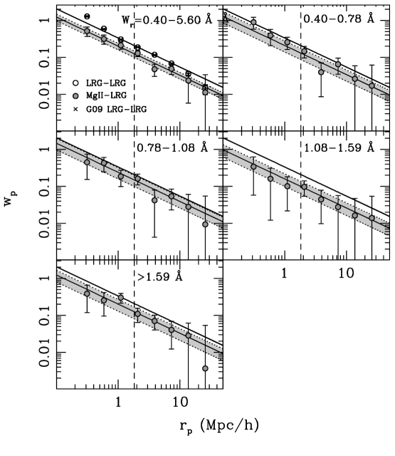
Figure 4: Two-point cross- and auto-correlation functions for the volume-limited sample of LRGs at $z=0.45-0.60$. In the top left panel, the LRG auto-correlation signal is represented by open circles while the Mg II–LRG cross-correlation is shown in solid grey circles. For comparison, we show the LRG–LRG auto-correlation function from G09 in crosses. To guide the eye, we included a thick solid line corresponding to the best-fit power-law model $f(x)=ax^{b}$ of the LRG auto-correlation signal at $r_{p}\mathrel{\hbox{\hbox to0.0pt{\hbox{\lower 3.0pt\hbox{$\sim$}}\hss}\hbox{\raise 2.0pt\hbox{$>$}}}}2$ $h^{-1}~{}{\rm Mpc}~{}$. The vertical dashed lines demarcate the small-scale (one-halo) $w_{p}$ from the large-scale (two-halo) $w_{p}$ on which the bias calculation is based. In this case, $b=-0.787$ and $a=0.335$. To facilitate the comparison between the clustering amplitude of absorbers and LRGs, we repeated this solid curve in all five remaining panels. The thin black curve corresponds to the best-fit power-law model of the cross-correlation function in which we fixed the power-law slope to the value derived for the LRG auto-correlation signal ($b=-0.787$). The dotted lines and and shaded areas correspond to the 1$-\sigma$ error bars on the amplitude $a$. The Mg II absorbers are divided in five bins according to the rest-frame equivalent width of the $\lambda 2796$ transition $W_{r}^{\lambda 2796}$. Each panel corresponds to a different $W_{r}^{\lambda 2796}$ bin labelled in the upper right corner. No correction for photometric redshifts is applied in this figure. The correction will be applied when estimating the relative bias of Mg II absorber hosts (see section 3.2). G09 showed that uncertainties in photometric redshifts of the LRGs decreases the clustering amplitude ratio between Mg II absorbers and the LRGs.

2.3.3 The errors on $w_{p}$

We consider two independent sources contributing to the errors in the measured $w_{p}$: cosmic variance and photometric redshift uncertainties. The contribution of cosmic variance can be estimated by using the jackknife resampling technique applied to the survey mask. The sky was separated into $N=192$ cells of similar survey area ($\approx 40$ deg²). The choice of the number of cells was obtained after running convergence tests on a varying number of cells (see G09 for more details). The cosmic variance estimate for each $r_{p,i}$ corresponds to the $i$th-diagonal element of the covariance matrix calculated with the jackknife method,

$${\rm COV}(w_{i},w_{j})=\frac{N-1}{N}\sum_{k=1}^{N}(w_{i}^{k}-\overline{w_{i}})(w_{j}^{k}-\overline{w_{j}})$$ (4)

where $k$ represents the iteration in which box $k$ was removed from the calculation. The mean value $\bar{w_{i}}$ was calculated for bin $i$ over all $w_{p}^{k}$’s. Although $r_{p}$ bins are correlated on large scales we consider only the diagonal elements of the covariance matrix when estimating the contribution of cosmic variance to the error on $w_{p}$.

The second source of errors comes from large uncertainties in the photometric redshifts of the galaxies. As discussed in G09, photometric redshift uncertainties affect $w_{p}$ in two distinct ways. The first effect is to lower the overall clustering amplitude by introducing uncorrelated pairs in the calculation (see section 3.2). The second effect is to add random noise in the calculation. This is particularly important for the inner $r_{p}$ bins which particularly suffer from an uncertainty on $z_{\rm ph}$ which translates into a large fractional uncertainty on $r_{p}$.

To estimate the random noise in $w_{p}$ as a result of photo-$z$ uncertainties, we followed the procedure described in G09. In brief, for each cross- and auto-correlation calculation, we generated 100 independent realizations of the LRG catalog by sampling the photo-$z$ distribution of each galaxy. We considered that each photo-$z$ distribution can be characterized by a normal distribution with $\sigma_{z}=0.03(1+z_{\rm ph})$ and a mean value $z_{\rm ph}$ (Collister et al., 2007). We then calculated $w_{p}$ for each realization and determined the photo-$z$ contribution to the error on $w_{p}$ by calculating the dispersion among these 100 realizations for each $r_{p}$ bin.

We found that while photometric redshift uncertainties can increase the random error by $\mathrel{\hbox{\hbox to0.0pt{\hbox{\lower 3.0pt\hbox{$\sim$}}\hss}\hbox{\raise 2.0pt\hbox{$<$}}}}20$% at $r_{p}\mathrel{\hbox{\hbox to0.0pt{\hbox{\lower 3.0pt\hbox{$\sim$}}\hss}\hbox{\raise 2.0pt\hbox{$<$}}}}1$$h^{-1}~{}{\rm Mpc}~{}$, the effect is negligible for larger values of $r_{p}$. Typically at these larger $r_{p}$ values, the increase is $<3$% for the LRG auto-correlation signal. Not surprisingly, the effect is smaller for the cross-correlation calculation since only one of the two pair members has photometric redshift. These findings are consistent with G09. Since the contribution of photo-$z$’s uncertainties is negligible on large scale where the clustering amplitude is calculated, we thus only considered cosmic variance in the error budget of $w_{p}$. Note however that photo-$z$’s also lowers the amplitude of the clustering signal and this effect is significant and is discussed in section 3.2.

2.3.4 Generating random LRGs and Mg II absorbers

The RA and DEC positions of each random LRG was generated using the ransack routine available through the Mangle software package. The redshifts of the random galaxies were determined by sampling the redshift distribution of the LRGs (see Figure 1). The number of random galaxies was determined after running convergence tests. As discussed in G09, having $\sim$ 10 times more random galaxies than the actual number of LRGs is sufficient to achieve convergence. Consequently, we generated a catalog of 4M random galaxies.

We randomly assigned the the RA and DEC positions of the random absorbers among the QSO sightlines that have been surveyed by ZM13 and S13 and fell within our survey mask. Of these sightlines, 63,294 were found within our spectroscopic survey mask. The redshift of each random Mg II was determined by sampling the redshift distribution of the absorber data while $W_{r}^{\lambda 2796}$ was assigned by sampling the distribution $dN/W_{r}\propto\exp(-W_{r}/W_{*})$ where $W_{*}$ is the typical absorber strength given by equation (5) in ZM13.

To allocate a given random absorber to a QSO sightline, one has to consider two additional limitations. First, the absorber should be found at velocity separation $|\delta_{v}|>10,000$ $\rm{km\,s}^{-1}$ from the QSO redshift and outside of the Ly$\alpha$ forest. This effectively eliminates all QSO sightlines with $z_{\rm QSO}<0.45$ and $z_{\rm QSO}>2.67$. Second, the QSO spectra should have high enough $S/N$ to detect a random absorber of a given strength. This constraint becomes particularly important when generating random absorbers for the weak absorber bin ($W_{r}^{\lambda 2796}=0.40-0.78$Å).

To establish whether or not a given sightline could harbor a random absorber of strength $W_{r}^{\lambda 2796}$, we empirically determined the minimum $W_{r}^{\lambda 2796}$ ($W_{r,\rm min}$) that could be detected at a given $S/N$ by adopting the following procedure. First, we determined the median $S/N$ per pixel, $\langle S/N\rangle$, over the redshift range $z_{\rm Mg\,II}=0.45-0.60$ for all QSO spectra in the Schneider et al. (2010) catalog. Next, we compared the strength of the Mg II absorbers listed in S13 with $\langle S/N\rangle$. The results are shown in Figure 3. We computed a 3rd-order polynomial fit to the bottom 5th-percentile of the $W_{r}^{\lambda 2796}$ distribution and interpret this fit as the minimum absorber strength, $W_{r,\rm min}(S/N)$, that could be detected given $\langle S/N\rangle$. The fit is shown by the solid line in Figure 3. Note that the value of $W_{r,\rm min}(S/N)$ corresponds approximately to a 2.5-$\sigma$ detection across the whole range of $\langle S/N\rangle$ considered. A random absorber of strength $W_{r}^{\lambda 2796}>W_{r,\rm min}$ could be detected and is included in our random absorber catalog. We repeated the procedures described above until we collected a sample of 100K random absorbers. We adopted this number of random absorbers after performing convergence tests, as described in G09.

3 Results

In this section, we present the projected two-point cross-correlation functions LRG–Mg II along with the LRG auto-correlation function for a volume-limited sample of LRGs at $z=0.45-0.60$. We explored the dependence of the clustering signal on $W_{r}^{\lambda 2796}$ by computing the LRG–Mg II cross-correlation for five $W_{r}^{\lambda 2796}$ bins with each bin having a similar number of absorbers. A summary of each calculation, including the adopted $W_{r}^{\lambda 2796}$ binning, the number of absorbers and LRGs along with the number of $D_{a}D_{g}$ pairs found in the first $r_{p}$ bin is presented in Table 1.

In Figure 4, we show the auto- and cross-correlation functions. In the top left panel, we show the LRG–LRG auto-correlation function in open circles. The error bars on the auto-correlation function are typically smaller than the size of the symbol. We calculated the best-fit power law model $f(x)=ax^{b}$ of the auto-correlation signal at $r_{p}\geq$ 2 $h^{-1}~{}{\rm Mpc}~{}$ and displayed the result as the thick solid line. We limited the fit to data points in the two-halo regime where the bias is determined. As discussed in Zehavi et al. (2004), correlation functions of galaxies display departures from power law models, especially at large separations. In the LRG auto-correlation function, this departure is more pronounced at $r_{p}>10$ $h^{-1}~{}{\rm Mpc}~{}$ and demonstrates the limitation of using such power law fits to determine the bias of galaxies and absorber hosts. In grey circles, we show the LRG–Mg II cross-correlation signal. We also adopted a power-law model for the cross-correlation function, but we fixed the slope to the value obtained for the LRGs ($b=-0.787$). The thin black line and the shaded areas correspond to the best-fit and 1-$\sigma$ errors on the amplitude $a$. Note that the best-fit power-law models are only shown to guide the eye and do not enter in the calculation of the relative bias of absorber hosts. The other five panels display the cross-correlation signals for the five $W_{r}^{\lambda 2796}$ bins considered. The range of $W_{r}^{\lambda 2796}$ for each bin is labeled in the upper-right corner of each panel. In all panels, the error bars on $w_{p}$ correspond to cosmic variance, estimated using the jackknife resampling technique (see section 2.4.3). Note that the data points shown in Figure 4 have not been corrected for the systematic effects of photometric redshifts on the clustering amplitude. These considerations will enter in the calculation of the relative bias of absorber hosts and are discussed in section 3.2.

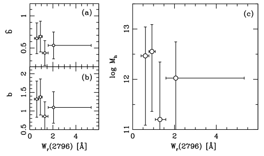
Figure 5: (a) Relative bias of Mg II hosts derived from the direct ratio method for points at $r_{p}\geq 2$$h^{-1}~{}{\rm Mpc}~{}$. We show the results for the four $W_{r}^{\lambda 2796}$ bins considered in this analysis. (b) Absolute bias of Mg II absorber hosts. To compute the bias, we adopted the bias of LRGs $b_{g}=2.023\pm 0.006$, as measured in G09. (c) In open circles, we show halo masses derived by inverting the $b(M)$ relationship. Note that the lower error-bar on four of the five $W_{r}^{\lambda 2796}$ bins are arbitrary. This occurs when the lower error bar reaches $b\approx 0.7$ giving us no constraint on the halo mass. The points represent the median of the $W_{r}^{\lambda 2796}$ distribution in each bin and the error bars on $W_{r}^{\lambda 2796}$ represent the extent of each bin.

At $r_{p}\mathrel{\hbox{\hbox to0.0pt{\hbox{\lower 3.0pt\hbox{$\sim$}}\hss}\hbox{\raise 2.0pt\hbox{$>$}}}}$ 2 $h^{-1}~{}{\rm Mpc}~{}$, where LRG–LRG and Mg II–LRG pairs are probing distinct dark matter halos (i.e., in the two-halo regime), the weakest absorbers ($W_{r}^{\lambda 2796}<1.08$Å) have the largest cross-correlation amplitude similar to the LRG auto-correlation signal. In contrast, absorbers in the bin $W_{r}^{\lambda 2796}=1.08-1.59$Å show, on average, the lowest clustering amplitude on large scales.

3.1 Theoretical framework on bias and halo mass determination

Here we provide a brief discussion of the theoretical framework behind the determination of the Mg II absorber host bias and halo mass from the projected two-point correlation function. A more detailed overview can be found in Berlind & Weinberg (2002), Zheng (2004), and Tinker et al. (2005).

The bias of dark matter halos of mass $M$ is the ratio of the real-space two-point correlation function of these dark matter halos, $\xi_{h}(M,r)$, and the dark matter auto-correlation function $\xi_{m}(r)$

$$b_{h}^{2}(M,r)=\frac{\xi_{h}(M,r)}{\xi_{m}(r)}\;.$$ (5)

In practice, we compute the projected two-point correlation statistics by integrating the real-space correlation function along the line-of-sight ($\pi$) direction

$$w_{p}(r_{p})=\int_{l}\xi(r_{p},\pi)d\pi\;.$$ (6)

The LRG–LRG auto-correlation signal $\xi_{gg}$ can be decomposed into a mass dependent $b_{g}^{2}(M_{g})$ and scale dependent $f_{g}^{2}(r)$ term

$$\xi_{gg}(M_{g},r)=b_{g}^{2}(M_{g})f_{g}^{2}(r)\xi_{m}(r)$$ (7)

where $M_{g}$ is the bias-weighted mean halo mass. Similarly, the cross-correlation absorber–galaxy term can be written as

$$\xi_{ga}(M_{g},M_{a},r)=b_{g}(M_{g})b_{a}(M_{a})f_{g}(r)f_{a}(r)\xi_{m}(r),$$ (8)

where the terms with subscript $a$ refer to the absorbers. On large scales and for the halo masses considered in this paper, the scale dependence of $b_{h}^{2}(M,r)$, $f(r)$, is almost independent of halo mass and is divided out when computing the relative bias of absorber hosts, $\hat{b}$. Consequently, one can write

$$\hat{b}\equiv\frac{b_{a}(M_{a})}{b_{g}(M_{g})}=\frac{\xi_{ga}(r)}{\xi_{gg}(r)}=\frac{w_{ag}(r_{p})}{w_{gg}(r_{p})}$$ (9)

where $\hat{b}$ is the scale-independent relative bias of absorber hosts $a$ with respect to a population of galaxies $g$. In other words, $\hat{b}$ can be calculated from the ratio of the projected two-point correlation functions $w$ on large scales. From $\hat{b}$, the bias (and mass) of the absorber hosts can be derived if the absolute bias of the tracer galaxy population ($b_{g}$) is known. For this purpose, we adopted the same galaxy bias as in G09. Since the LRG selection criteria and redshift range are the same as G09, the auto-correlation signal of LRGs should, in principle be the same. We verified that this was the case. In the upper-left panel of Figure 4, we show the LRG auto-correlation signal of G09 in crosses. As expected, the differences from G09 are negligible. We thus adopted the bias value of $b_{g}=2.023\pm 0.006$ as found by G09.

3.2 Calculating the relative bias

Before calculating the relative bias of Mg II absorber hosts, it is important to consider the effects of photometric redshifts on the clustering amplitude and bias measurements. LRGs typically have photo-$z$ accuracy of $\sigma_{z}\approx 0.03(1+z_{\rm ph})$. Large uncertainties on the galaxy redshifts affect the clustering signal in two different ways. Since the redshifts are uncertain, the angular diameter distance is uncertain too, introducing uncertainties in the projected co-moving separations between LRGs and Mg II absorbers and effectively “smoothing” out sharp features present in the intrinsic two-point correlation signal. As discussed in section 2.4.3, this source of uncertainty mostly affects the inner bins of the correlation function and is negligible at $r_{p}\mathrel{\hbox{\hbox to0.0pt{\hbox{\lower 3.0pt\hbox{$\sim$}}\hss}\hbox{\raise 2.0pt\hbox{$>$}}}}$ 2 $h^{-1}~{}{\rm Mpc}~{}$where the clustering amplitude is measured.

Furthermore, photometric redshift errors effectively broadens the redshift range included in the calculation and adds uncorrelated galaxy–Mg II pairs in the calculation. This effect results in a systematic lowering of the amplitude of the clustering signal. G09 addressed this issue by calculating the projected clustering signal on mock LRG distributions. Their mock catalog was produced by populating dark matter halos of an $N-$body simulation with a halo occupation distribution function determined from a spectroscopic LRG sample. Then the redshift of each galaxy was perturbed to mimic the effects of photometric redshifts and the authors re-calculated the two-point correlation statistics. In a nutshell, G09 found that the MgII–LRG cross-correlation amplitude on large scales ($>1$ $h^{-1}~{}{\rm Mpc}~{}$) is reduced by a factor 0.79$\pm$0.02 compared to what is found for a spectroscopic sample of LRGs while the LRG–LRG auto-correlation amplitude is reduced by 0.71$\pm$0.01. Consequently, we determined the relative bias, $\hat{b}$, by multiplying the uncorrected $\hat{b}$ values by the correction factor $\mathcal{C}=0.90\pm 0.02$. Hereafter, all $\hat{b}$ and absolute bias measurements $b$ are corrected for this systematic effect introduced by photometric redshifts.

In G09, they discussed the direct ratio (DR) method to calculate the relative bias of absorber hosts. This technique employs the weighted mean ratio of all data points at $r_{p}\mathrel{\hbox{\hbox to0.0pt{\hbox{\lower 3.0pt\hbox{$\sim$}}\hss}\hbox{\raise 2.0pt\hbox{$>$}}}}2$ $h^{-1}~{}{\rm Mpc}~{}$ to obtain $\hat{b}$

$$\hat{b}=\sum_{i=4}^{8}\omega_{i}\frac{w_{ag,i}}{w_{gg,i}}\times\mathcal{C}$$ (10)

where the weights, $\omega_{i}$ are given by

$$\omega_{i}=\frac{w_{ag,i}}{\sigma_{i}^{2}w_{gg,i}}\;.$$ (11)

The index $i$ denotes the $r_{p}$ bin and $\sigma_{i}$ is the error on $w_{ag,i}/w_{gg,i}$ using error propagation technique as is the error on $\hat{b}$ (see G09). In Table 2, we provide estimates for the relative bias $\hat{b}$, bias $b$, and halo masses for each one of the five $W_{r}^{\lambda 2796}$ bins considered and the entire Mg II sample.

3.3 Absolute bias and halo mass

As discussed in section 3.1, the halo mass of absorber hosts could be obtained simply by inverting the $b(M)$ relationship. We refer to this method as bias-inverted halo mass. Moreover, one can estimate halo masses by integrating the bias-weighted halo mass function down in mass until the bias value reaches $b$. The minimum halo mass corresponding to $b$ can thus be used as a lower-limit in the integral of the halo mass function. This bias-weighted halo mass estimate is simply derived by integrating the mass-weighted halo mass function using this lower-limit.

These two techniques were discussed in details in G09. The authors show that the methods give halo mass estimates within 0.1 dex of each other for both LRGs and Mg II absorber hosts. Consequently, we followed the G09 methodology and used the bias-inverted masses as our Mg II hosts mass estimates.

In Figure 5, we show the relative bias, bias, and halo masses of Mg II absorber hosts for the five $W_{r}^{\lambda 2796}$ bins considered. Except for the weakest absorbers, the lower error bars we quoted on the halo masses are arbitrary. This lack of constraints arises because when the lower error bar on the bias reaches 0.7, there is no constraint on the halo mass. In fact, $b(M)$ reaches a minimum value of $\approx 0.7$ and becomes nearly independent of halo mass at log $M_{h}\mathrel{\hbox{\hbox to0.0pt{\hbox{\lower 3.0pt\hbox{$\sim$}}\hss}\hbox{\raise 2.0pt\hbox{$<$}}}}9$ (e.g., Tinker et al. 2008).

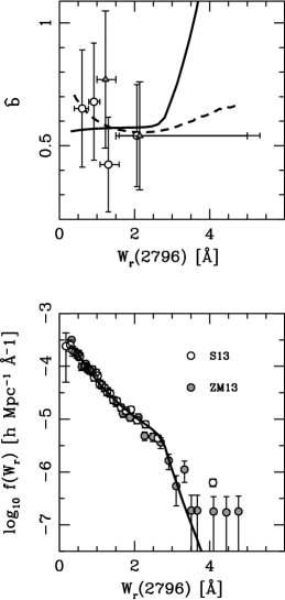
Figure 6: Top: Comparison between the relative bias estimates of Mg II absorber hosts and the predictions from a simple model in which the gas distribution follows an isothermal profile (see section 4 for further details). In open circles are the $\hat{b}$ values found in this paper. In grey triangles we show the results from G09. The solid line corresponds to our best-fit model. Interestingly, this model predicts a monotonically increasing $b$–$W_{r}$ relation. We also present a direct comparison between the predictions of the “transition” model from Tinker & Chen (2008) (TC08) in dashed curve (see section 4 for further details). This transition models predicts an anti-correlation between $b$ and $W_{r}$ and is in better agreement with our data, especially for the weakest $W_{r}$ bins. Bottom: Comparison between the best-fit model and the frequency distribution function of absorbers, $f(W_{r})$, measured by S13 (open circles) in the redshift range $z_{\rm Mg\,II}=0.45-0.60$. We also plotted the ZM13 $f(W_{r})$ values in grey circles over the range $z_{\rm Mg\,II}=0.43-0.55$ for comparison. Because of the small $f(W_{r})$ error bars for points at $W_{r}\mathrel{\hbox{\hbox to0.0pt{\hbox{\lower 3.0pt\hbox{$\sim$}}\hss}\hbox{\raise 2.0pt\hbox{$<$}}}}2$Å, the $\chi^{2}$ is driven by the weak $W_{r}$ bins. The model tends to underestimate $f(W_{r})$ for strong absorbers although a larger covering fraction for massive halos or a higher $A_{W_{0}}$ would over predict the number of weaker systems while flattening the overall $f(W_{r})$ slope. For 32 degrees of freedom, this model has a reduced $\chi^{2}$, $\chi_{r}^{2}=1.81$ which has an associated $P$-value $P=0.003$. Accordingly, this simple model can be rejected at a $\approx 2.8\sigma$ (one-sided) confidence level.

Table 1: Description of the cross-correlation calculations

$W_{r}^{\lambda 2796}$ [Å]	N${}_{\rm Mg\,II}$	NLRGs	DD pairs (1st bin)
All	2211	333334	130
$0.40-0.78$	559	333334	36
$0.78-1.08$	531	333334	26
$1.08-1.59$	564	333334	25
$>1.59$	557	333334	24

4 Discussion

We presented the cross-correlation function of Mg II absorbers with respect to a volume-limited sample of LRGs at $z=0.45-0.60$ using the SDSS DR7 galaxy and absorber catalogs. We benefited from an absorber catalog four times larger and an increase of 70% in the number of LRGs compared to the samples used in G09. We extended the clustering analysis to weaker absorbers with $W_{r}^{\lambda 2796}<1$Å that were excluded from the G09 analysis.

The clustering signal of Mg II absorbers was calculated in four $W_{r}^{\lambda 2796}$ bins of roughly equal number of absorbers spanning the range $W_{r}^{\lambda 2796}=0.4-5.6$Å. On average, stronger absorbers with $W_{r}^{\lambda 2796}>1$Å reside in less massive halos than weaker ones.

Table 2: Relative bias, absolute bias, and halo mass estimates of Mg II absorber hosts

$W_{r}^{\lambda 2796}$ [Å]	$\hat{b}$	$b$	$\langle\log M_{h}\rangle$
All	0.56 $\pm$ 0.12	1.14 $\pm$ 0.23	$12.1^{+0.4}_{-0.7}$
$0.4-0.78$	0.65 $\pm$ 0.24	1.32 $\pm$ 0.48	12.5${}^{+0.6}_{-1.4}$
$0.78-1.08$	0.68 $\pm$ 0.24	1.38 $\pm$ 0.48	12.6${}^{+0.5}_{-1.2}$
$1.08-1.59$	0.42 $\pm$ 0.19	0.86 $\pm$ 0.39	11.2+1.1
$>1.59$	0.54 $\pm$ 0.21	1.10 $\pm$ 0.42	12.0+0.7

The observed $b$–$W_{r}^{\lambda 2796}$ relation offers a statistical characterization of the origin of the Mg II absorbers as a whole, but the interpretation requires a comprehensive model of halo gas content as a function of halo mass. Similarly, the frequency distribution function $f(W_{r})$ of absorbers, namely the number of absorbers per unit $W_{r}$ per unit comoving length, also provides important constraints on halo gas models. We thus compared these two datasets with the predictions of a simple analytical model in which the Mg II gas is distributed in dark matter halos according to an isothermal profile. In this model, the gas clumps are distributed according to an isothermal profile of finite radial extent. This radius is denoted by $R_{\rm gas}$, the gaseous radius of the halo. In our model, the value of $R_{\rm gas}$ is set to $R_{\rm gas}=1/3\times R_{\rm vir}$ where $R_{\rm vir}$ is the virial radius of the dark matter halo following Chen et al. (2010). For example, a typical $L_{*}$ galaxy with halo mass $\sim 10^{12}$ $h^{-1}\,{\rm M}_{\odot}$ at $z\sim 0.25$ has $R_{\rm gas}=75$ $h^{-1}~{}{\rm kpc}~{}$(Chen et al., 2010). The total absorption equivalent width is the sum over all clumps encountered along the sightline and thus corresponds to the integral of the isothermal profile along a given sightline located at impact parameter $s$

$$W_{r}(s,M)=A_{W}\frac{2\mathcal{G}_{0}}{\sqrt{s^{2}+a_{h}^{2}}}\arctan\sqrt{\frac{R_{\rm gas}^{2}-s^{2}}{s^{2}+a_{h}^{2}}}$$ (12)

where $a_{h}$ is the core radius of the isothermal profile, $A_{W}$ is the mean absorption equivalent width per unit surface mass density of the cold gas and $\mathcal{G}_{0}$ is

$$\mathcal{G}_{0}=\frac{M(<R_{\rm gas})/4\pi}{R_{\rm gas}-a_{h}\arctan(R_{\rm gas}/a_{h})}\;.$$ (13)

Following Tinker & Chen (2008, hereafter TC08), we set $a_{h}=0.2R_{\rm gas}$ and adopted a power-law for $A_{W}$

$$A_{W}(M)=A_{W_{0}}\bigg{(}\frac{M}{10^{12}h^{-1}M_{\odot}}\bigg{)}^{-0.2}~{}[h^{-1}\rm{\AA}~{}\rm{cm}^{2}~{}\rm{g}^{-1}]$$ (14)

where $A_{W_{0}}$ is a free parameter independent of halo mass. The slope of this power-law corresponds to the best-fit value of TC08. The frequency distribution function can be written as

$$f(W_{r})\equiv\frac{d^{2}N}{dW_{r}dl}=\int dM\frac{dn}{dM}\sigma_{g}(M)P(W_{r}|M)$$ (15)

where $dn/dM$ is the halo mass function (Warren et al. 2006), $\sigma_{g}(M)=\pi R_{\rm gas}^{2}$ is the gas cross section and $P(W_{r}|M)$ is the probability that a halo of mass $M$ hosts an absorber of strength $W_{r}$. In turn, $P(W_{r}|M)$ can be written as :

$$P(W_{r}|M)=\kappa_{g}(M)\frac{2s(W_{r}|M)}{R_{\rm gas}^{2}}\frac{ds}{dW_{r}}$$ (16)

(see equation 10 of TC08). In this expression, the impact parameter $s(W_{r}|M)$ is found by inverting equation 12 which is performed numerically. The derivative of $s$ with respect to $dW_{r}$, $ds/dW_{r}$, is calculated following equation 11 in TC08. In equation 16, $\kappa_{g}(M)$ is the gas covering fraction. We adopted a double power law to account for the mass dependence of $\kappa$

$$\kappa(M)=\begin{cases}\kappa_{12}(M/10^{12})^{\gamma},&\mbox{if }M\leq 10^{12}\mbox{$h^{-1}\,{\rm M}_{\odot}$}\\ \kappa_{12}(M/10^{12})^{\alpha},&\mbox{if }M>10^{12}\mbox{$h^{-1}\,{\rm M}_{\odot}$}\end{cases}$$ (17)

Following the empirical findings of Chen et al. (2010), we assigned $\kappa_{12}=0.7$ which corresponds to the covering fraction of $W_{r}^{\lambda 2796}>0.3$ Å absorbers in $L_{*}$-galaxy halos. Both slopes $\alpha$ and $\gamma$ are free parameters.

In addition to $f(W_{r})$, the model described above allows us to predict the $b$–$W_{r}$ relation. The bias corresponds to the mean halo bias weighted by the probability of finding an absorber $W_{r}$ in a halo of mass $M$

$$b=\frac{1}{f(W_{r})}\int dM\frac{dn}{dM}\sigma_{g}(M)b_{h}(M)P(W_{r}|M)$$ (18)

where $b_{h}$ is the halo bias taken from Tinker et al. (2008).

In summary, this model has three free parameters: $A_{W_{0}}$, $\alpha$, and $\gamma$. We generated a grid of models by varying these three parameters independently and we compared our model predictions for $f(W_{r})$ and $b$ with the empirical data of S13 in the range $z_{\rm Mg\,II}=0.45-0.60$ and the bias data points of Figure 5a. In addition, we plotted in grey the ZM13 $f(W_{r})$ data over the redshift range $z_{\rm Mg\,II}=0.43-0.55$ for comparison. For each model, we computed a $\chi^{2}$ goodness-of-fit test

$$\chi^{2}=\chi_{b}^{2}+\chi_{f}^{2}=\sum_{i=0}^{4}\frac{(b_{i}-\bar{b}_{i})^{2}}{\sigma_{b_{i}}^{2}}+\sum_{j=0}^{31}\frac{(f_{j}-\bar{f}_{j})^{2}}{\sigma_{f_{j}}^{2}}$$ (19)

where $\chi_{b}^{2}$ and $\chi_{f}^{2}$ correspond to the values from the bias and frequency distribution function. The parameters $\bar{b}$ and $\bar{f}$ are the model predictions for the bias and frequency distribution function respectively. Because of the larger number of datapoints of the frequency data (31 vs 4), $\chi_{f}^{2}$ will dominate over $\chi_{b}^{2}$ for most values of $(A_{W_{0}},\alpha,\gamma)$. The best-fit model has $\chi^{2}=57.9$ with $\chi_{b}^{2}=0.96$ and $\chi_{f}^{2}=56.97$ The corresponding best-fit parameters are $(126,-1.40,2.18)$. For a $10^{13}\mbox{$h^{-1}\,{\rm M}_{\odot}$}$ halo, this model predicts $\kappa=0.03$, which is lower than the value obtained by Gauthier & Chen (2011) for LRG halos ($\kappa_{\rm LRG}=0.22\pm 0.13$). We show the best-fit model in Figure 6. Because of the small $f(W_{r})$ error bars for points at $W_{r}\mathrel{\hbox{\hbox to0.0pt{\hbox{\lower 3.0pt\hbox{$\sim$}}\hss}\hbox{\raise 2.0pt\hbox{$<$}}}}2$Å, $\chi_{f}^{2}$ is driven by the weak $W_{r}$ bins. The model tends to underestimate $f(W_{r})$ for strong absorbers although a larger $\kappa$ for massive halo or a larger $A_{W_{0}}$ would over predict the number of weaker systems while flattening the overall $f(W_{r})$ slope. Interestingly, this model predicts a monotonically increasing $b$–$W_{r}$ relation. For 32 degrees of freedom, the reduced $\chi^{2}$ is $\chi_{r}^{2}=1.81$ which has an associated $P$-value of $P\approx 0.003$. Accordingly, this simple model can be rejected at a $\approx 2.8\sigma$ (one-sided) confidence level.

In contrast with the simple model presented above, TC08 also developed a halo occupation distribution model (HOD) in which they introduced a transition mass scale of $\sim 3\times 10^{11}$ $h^{-1}\,{\rm M}_{\odot}$ above which a shock develops and reduce the amount of Mg II absorbing gas within the shock radius. This transition mass scale was motivated by recent hydrodynamical simulations of galaxy formation showing two distinct channels of gas accretion for halos above and below the transition scale (e.g. Kereš et al. 2009), although the conclusions drawn from these early studies are now being challenged by recent hydrodynamical simulations (e.g., Nelson et al. 2013). TC08 showed that their model predicts near unity covering fraction of Mg II absorbing gas over a wide range of halo masses, suggesting that Mg II absorbers are probing an unbiased sample of galaxies, not preferentially selected for their recent star formation activity. Although this “transition” model provides a better fit to $f(W_{r})$, the most important differences occur in the $b$–$W_{r}$ relationship. Because of the shock radius developing in massive halos, the transition model predicts a suppressed contribution from massive halos yielding a lower $b$ for stronger absorbers. This results in an overall $b$–$W_{r}$ anti-correlation. In Figure 6 we show a direct comparison between the relative bias and the model predictions taken from TC08. The best-fit TC08 “transition” model is shown in dashed and provides a better fit to the bias data although most of the discriminative power lies in the weakest $W_{r}$ bin.

The bias data shown in Figure 5 suggest a possible flattening or upturn in the $b$–$W_{r}$ relation for absorbers with $W_{r}^{\lambda 2796}\mathrel{\hbox{\hbox to0.0pt{\hbox{\lower 3.0pt\hbox{$\sim$}}\hss}\hbox{\raise 2.0pt\hbox{$>$}}}}1.59$Å. A similar, trend was also seen in Bouché et al. (2006) and Lundgren et al. (2009). These results are consistent with Gauthier (2013) who argue that ultra-strong Mg II absorbers with $W_{r}^{\lambda 2796}\mathrel{\hbox{\hbox to0.0pt{\hbox{\lower 3.0pt\hbox{$\sim$}}\hss}\hbox{\raise 2.0pt\hbox{$>$}}}}3$Å trace gas dynamics of the intragroup medium. Gauthier (2013) estimated halo masses of $\log M_{h}=12-13.3$ for the galaxy groups presented in their paper and in Nestor et al. (2011).

Similar group environments have also been found around $W_{r}^{\lambda 2796}\approx 2$Å absorbers at intermediate redshifts (Whiting et al., 2006; Kacprzak et al., 2010).

Nevertheless, the SDSS-III Baryon Oscillation Spectroscopic Survey (BOSS) is collecting a large sample of spectroscopically identified LRGs with a redshift precision of $dz<0.0005$ instead of $dz\sim 0.05$. The availablity of a spectroscopic LRG sample offers an exciting opportunity to study the real-space clustering signal of Mg II absorbers and to examine the two-point function on small scales ($<$1Mpc). These new measurements will provide further insights into large-scale motion of cool gas uncovered by Mg II and allow a detailed investigation of the cool halo gas content of massive halos hosting the LRGs.

References

- Adelberger et al. (2003) Adelberger K. L., Steidel C. C., Shapley A. E., Pettini M., 2003, ApJ, 584, 45
- Barton & Cooke (2009) Barton E. J., Cooke J., 2009, AJ, 138, 1817
- Bechtold & Ellingson (1992) Bechtold J., Ellingson E., 1992, ApJ, 396, 20
- Bergeron & Boissé (1991) Bergeron J., Boissé P., 1991, A&A, 243, 344
- Bergeron & Stasińska (1986) Bergeron J., Stasińska G., 1986, A&A, 169, 1
- Berlind & Weinberg (2002) Berlind A. A., Weinberg D. H., 2002, ApJ, 575, 587
- Blake et al. (2008) Blake C., Collister A., Lahav O., 2008, MNRAS, 385, 1257
- Blanton et al. (2005) Blanton M. R., Schlegel D. J., Strauss M. A., Brinkmann J., Finkbeiner D., Fukugita M., Gunn J. E., Hogg D. W., Ivezić Ž., Knapp G. R., Lupton R. H., Munn J. A., Schneider D. P., Tegmark M., Zehavi I., 2005, AJ, 129, 2562
- Bouché & Lowenthal (2004) Bouché N., Lowenthal J. D., 2004, ApJ, 609, 513
- Bouché et al. (2004) Bouché N., Murphy M. T., Péroux C., 2004, MNRAS, 354, L25
- Bouché et al. (2006) Bouché N., Murphy M. T., Péroux C., Csabai I., Wild V., 2006, MNRAS, 371, 495
- Bowen et al. (1995) Bowen D. V., Blades J. C., Pettini M., 1995, ApJ, 448, 634
- Bullock et al. (2002) Bullock J. S., Wechsler R. H., Somerville R. S., 2002, MNRAS, 329, 246
- Chen et al. (2010) Chen H.-W., Helsby J. E., Gauthier J.-R., Shectman S. A., Thompson I. B., Tinker J. L., 2010, ApJ, 714, 1521
- Chen & Mulchaey (2009) Chen H.-W., Mulchaey J. S., 2009, ApJ, 701, 1219
- Chen & Tinker (2008) Chen H.-W., Tinker J. L., 2008, ApJ, 687, 745
- Chen et al. (2010) Chen H.-W., Wild V., Tinker J. L., Gauthier J.-R., Helsby J. E., Shectman S. A., Thompson I. B., 2010, ApJ, 724, L176
- Churchill et al. (2005) Churchill C. W., Kacprzak G. G., Steidel C. C., 2005, in Williams P., Shu C.-G., Menard B., eds, IAU Colloq. 199: Probing Galaxies through Quasar Absorption Lines MgII absorption through intermediate redshift galaxies. pp 24–41
- Churchill et al. (2003) Churchill C. W., Vogt S. S., Charlton J. C., 2003, AJ, 125, 98
- Collister et al. (2007) Collister A., Lahav O., Blake C., Cannon R., Croom S., Drinkwater M., Edge A., Eisenstein D., Loveday J., Nichol R., Pimbblet K., de Propris R., Roseboom I., Ross N., Schneider D. P., Shanks T., Wake D., 2007, MNRAS, 375, 68
- Cooke et al. (2006) Cooke J., Wolfe A. M., Gawiser E., Prochaska J. X., 2006, ApJ, 652, 994
- Cooksey et al. (2013) Cooksey K. L., Kao M. M., Simcoe R. A., O’Meara J. M., Prochaska J. X., 2013, ApJ, 763, 37
- Daddi et al. (2003) Daddi E., Röttgering H. J. A., Labbé I., Rudnick G., Franx M., Moorwood A. F. M., Rix H. W., van der Werf P. P., van Dokkum P. G., 2003, ApJ, 588, 50
- Davis & Peebles (1983) Davis M., Peebles P. J. E., 1983, ApJ, 267, 465
- Gauthier (2013) Gauthier J.-R., 2013, ArXiv e-prints
- Gauthier & Chen (2011) Gauthier J.-R., Chen H.-W., 2011, MNRAS, 418, 2730
- Gauthier et al. (2010) Gauthier J.-R., Chen H.-W., Tinker J. L., 2010, ApJ, 716, 1263
- Hamilton & Tegmark (2004) Hamilton A. J. S., Tegmark M., 2004, MNRAS, 349, 115
- Hartley et al. (2013) Hartley W. G., Almaini O., Mortlock A., Conselice C. J., Grützbauch R., Simpson C., Bradshaw E. J., Chuter R. W., Foucaud S., Cirasuolo M., Dunlop J. S., McLure R. J., Pearce H., 2013, ArXiv e-prints
- Hewett & Wild (2010) Hewett P. C., Wild V., 2010, MNRAS, 405, 2302
- Kacprzak et al. (2008) Kacprzak G. G., Churchill C. W., Steidel C. C., Murphy M. T., 2008, AJ, 135, 922
- Kacprzak et al. (2010) Kacprzak G. G., Murphy M. T., Churchill C. W., 2010, MNRAS, 406, 445
- Kereš et al. (2009) Kereš D., Katz N., Fardal M., Davé R., Weinberg D. H., 2009, MNRAS, 395, 160
- Lanzetta & Bowen (1990) Lanzetta K. M., Bowen D., 1990, ApJ, 357, 321
- Lundgren et al. (2009) Lundgren B. F., Brunner R. J., York D. G., Ross A. J., Quashnock J. M., Myers A. D., Schneider D. P., Al Sayyad Y., Bahcall N., 2009, ApJ, 698, 819
- Nelson et al. (2013) Nelson D., Vogelsberger M., Genel S., Sijacki D., Kereš D., Springel V., Hernquist L., 2013, MNRAS, 429, 3353
- Nestor et al. (2011) Nestor D. B., Johnson B. D., Wild V., Ménard B., Turnshek D. A., Rao S., Pettini M., 2011, MNRAS, 412, 1559
- Nielsen et al. (2013) Nielsen N. M., Churchill C. W., Kacprzak G. G., Murphy M. T., 2013, ArXiv e-prints
- Padmanabhan et al. (2008) Padmanabhan N., White M., Norberg P., Porciani C., 2008, ArXiv 0802.210
- Rao et al. (2006) Rao S. M., Turnshek D. A., Nestor D. B., 2006, ApJ, 636, 610
- Ross et al. (2009) Ross N. P., Shen Y., Strauss M. A., Vanden Berk D. E., Connolly A. J., Richards G. T., Schneider D. P., Weinberg D. H., Hall P. B., Bahcall N. A., Brunner R. J., 2009, ApJ, 697, 1634
- Rubin et al. (2010) Rubin K. H. R., Weiner B. J., Koo D. C., Martin C. L., Prochaska J. X., Coil A. L., Newman J. A., 2010, ApJ, 719, 1503
- Schlegel et al. (1998) Schlegel D. J., Finkbeiner D. P., Davis M., 1998, ApJ, 500, 525
- Seyffert et al. (2013) Seyffert E. N., Cooksey K. L., Simcoe R. A., O’Meara J. M., Kao M. M., Prochaska J. X., 2013, ApJ, 779, 161
- Shen et al. (2011) Shen Y., Richards G. T., Strauss M. A., Hall P. B., Schneider D. P., Snedden S., Bizyaev D., Brewington H., Malanushenko V., Malanushenko E., Oravetz D., Pan K., Simmons A., 2011, ApJS, 194, 45
- Steidel et al. (1994) Steidel C. C., Dickinson M., Persson S. E., 1994, ApJ, 437, L75
- Swanson et al. (2008) Swanson M. E. C., Tegmark M., Hamilton A. J. S., Hill J. C., 2008, MNRAS, 387, 1391
- Thomas et al. (2011) Thomas S. A., Abdalla F. B., Lahav O., 2011, MNRAS, 412, 1669
- Tinker et al. (2008) Tinker J., Kravtsov A. V., Klypin A., Abazajian K., Warren M., Yepes G., Gottlöber S., Holz D. E., 2008, ApJ, 688, 709
- Tinker & Chen (2008) Tinker J. L., Chen H.-W., 2008, ApJ, 679, 1218
- Tinker et al. (2005) Tinker J. L., Weinberg D. H., Zheng Z., Zehavi I., 2005, ApJ, 631, 41
- Trainor & Steidel (2012) Trainor R. F., Steidel C. C., 2012, ApJ, 752, 39
- Tripp & Bowen (2005) Tripp T. M., Bowen D. V., 2005, in Williams P., Shu C.-G., Menard B., eds, IAU Colloq. 199: Probing Galaxies through Quasar Absorption Lines The connections between QSO absorption systems and galaxies: low-redshift observations. pp 5–23
- Weiner et al. (2009) Weiner B. J., Coil A. L., Prochaska J. X., Newman J. A., Cooper M. C., Bundy K., Conselice C. J., Dutton A. A., Faber S. M., Koo D. C., Lotz J. M., Rieke G. H., Rubin K. H. R., 2009, ApJ, 692, 187
- Whiting et al. (2006) Whiting M. T., Webster R. L., Francis P. J., 2006, MNRAS, 368, 341
- Zehavi & al. (2002) Zehavi I., al. 2002, ApJ, 571, 172
- Zheng (2004) Zheng Z., 2004, ApJ, 610, 61
- Zhu & Ménard (2013) Zhu G., Ménard B., 2013, ApJ, 770, 130