Statistical Post-Processing of Forecasts for Extremes Using Bivariate Brown-Resnick Processes with an Application to Wind Gusts

Abstract

To improve the forecasts of weather extremes, we propose a joint spatial model for the observations and the forecasts, based on a bivariate Brown-Resnick process. As the class of stationary bivariate Brown-Resnick processes is fully characterized by the class of pseudo cross-variograms, we contribute to the theorical understanding of pseudo cross-variograms refining the knowledge of the asymptotic behaviour of all their components and introducing a parsimonious, but flexible parametric model. Both findings are of interest in classical geostatistics on their own. The proposed model is applied to real observation and forecast data for extreme wind gusts at 119 stations in Northern Germany.

Keywords: bivariate random field, Matérn model, max-stable process, pseudo cross-variogram

1 Introduction

Spatial extremes may occur in various forms such us heavy rainfall, floods, heat waves or wind gusts. In view of their severe consequences, an adequate and precise forecast of these events is of great importance. However, the rareness of extreme events impedes any such task and, consequently, existing forecasts often lack accuracy. In meteorology, for example, forecasting extreme wind gusts, which are defined as peak wind speeds over a few seconds, is exacerbated by the short temporal and spatial ranges. Furthermore, numerical weather prediction (NWP) models provide estimates or diagnoses of wind gusts based on empirical knowledge only (cf. Brasseur, 2001). Although wind is a prognostic variable in NWP models, its values represents an average wind speed over a few minutes or longer depending on the grid spacing of the NWP model. Hence, post-processing procedures are needed that allow for an enhanced probabilistic forecast.

Occurring as limits of normalized pointwise maxima of stochastic processes, max-stable processes provide a suitable framework for the description of spatial extreme events, commonly used in environmental sciences (Coles, 1993; Coles and Tawn, 1996; Huser and Davison, 2014). Of particular interest is the subclass formed by Brown-Resnick processes which arise as limits of rescaled maxima of Gaussian processes (Brown and Resnick, 1977; Kabluchko et al., 2009; Kabluchko, 2011).

During the last years, max-stable processes have been frequently applied as models for spatial extremes in environmental sciences. For instance, Engelke et al. (2015) and Genton et al. (2015) recently used max-stable processes to model extreme wind speed observations. The model we propose will go one step further, also taking into account the forecasts in two different aspects: First and in contrast to Engelke et al. (2015) and Genton et al. (2015), we consider the mean forecast to get a normalized version of the extreme observations. Second, besides the observable variable of interest itself, the corresponding forecast is included as second variable yielding a bivariate max-stable process. Here, we will focus on the class of bivariate Brown-Resnick processes (cf. Molchanov and Stucki, 2013; Genton et al., 2015) to exploit the statistical relation between observable data and the corresponding forecast. Modeling the behavior of observational data, a sample from the distribution of the observations conditional on the forecast is supposed to provide more realistic results than the original forecast and thus will appear as an appropriate probabilistic post-processed forecast.

The paper is structured as follows: In Section 2, we present a univariate model for extreme observations, which may, in general, provide a first alternative to the original forecast. We introduce a model for the marginal distribution, i.e. the distribution of the observable variable of interest at a single location, motivating the normalization of its extremes by the mean forecast. The spatial dependence structure is incorporated into the model by the use of univariate Brown-Resnick processes. Section 3 is dedicated to the bivariate Brown-Resnick process which serves as a joint model for both the maximally observed and forecasted quantities. We deduce a necessary condition on the asymptotic behavior of the pseudo cross-variogram and provide a flexible cross-variogram model which leads to a stationary bivariate Brown-Resnick process. In Section 4, we describe how the model can be fitted to data. Based on this model, we propose a post-processing procedure which is presented in Section 5. Further, we provide tools to verify the procedure and the underlying models. Finally, the methods presented in Sections 4 and 5 are applied to real observation and forecast data for extreme wind gusts provided by the German’s National Meteorological Service, Deutscher Wetterdienst (DWD) (Section 6).

2 Modeling by a Univariate Random Field

In this section, we present a spatial model for the observed pointwise maximum $V_{\max}^{\rm obs}$ within a specific time period. To this end, we assume that, for each location and time period, the maximum $V_{\max}^{\rm obs}$ is based on observations at $N$ equidistant instants of times per period, that is, we have $V_{\max}^{\rm obs}=\max_{t=1,\ldots,N}V^{\rm obs}_{t}$ for $V_{1}^{\rm obs},\ldots,V_{N}^{\rm obs}\sim F_{\vartheta}$ for some parameter $\vartheta$. Here, the probability distributions $F_{\vartheta}$ are supposed to form a location-scale family with finite second moments, i.e.  $\vartheta=(m,s)\in\mathbb{R}\times(0,\infty)$ with $F_{(m,s)}(x)=F_{(0,1)}\left(\frac{x-m}{s}\right)$, $x\in\mathbb{R}$, and $F_{(0,1)}$ is standardized to mean zero and unit variance. We assume $\vartheta=(m,s)$ to be temporally constant at each location within the same time period, but allow the values to vary among different locations and different time periods. The values of $m$ and $s$ will essentially be estimated from the bulk of the distribution, not the tail, and thus, they can often be extracted accurately from forecasts. Within the same time period and at the same location, the observable variables $V_{1}^{\rm obs},\ldots,V_{N}^{\rm obs}$ are assumed to be subsequent $N$ elements of a stationary time series $(V_{t}^{\rm obs})_{t\in\mathbb{Z}}$. Furthermore, we assume that the standardized distribution $F_{(0,1)}$ belongs to the max-domain of attraction of some univariate extreme value distribution $G_{\xi}$, $\xi\in\mathbb{R}$, i.e. there are sequences $(a_{n})_{n\in\mathbb{N}}$, $a_{n}>0$, and $(b_{n})_{n\in\mathbb{N}}$, $b_{n}\in\mathbb{R}$, such that

$$F_{(0,1)}^{n}(a_{n}x+b_{n})\stackrel{{\scriptstyle n\to\infty}}{{\longrightarrow}}G_{\xi}(x),\quad 1+\xi x>0,$$

where

$$G_{\xi}(x)=\begin{cases}\exp(-(1+\xi x)^{-1/\xi}),&\xi\neq 0,\\ \exp(-\exp(-x)),&\xi=0,\end{cases}$$

for $1+\xi x>0$. As the second moment of $F_{(0,1)}$ is assumed to be finite, we have $\xi<0.5$. Under some conditions on the regularity and the dependence of the stationary sequence $V^{\rm obs}_{1},V^{\rm obs}_{2},\ldots$, we obtain that

$$\mathbb{P}\left(\frac{\max_{i=1,\ldots,n}V^{\rm obs}_{i}-m-\widetilde{b}_{n}s}{\widetilde{a}_{n}s}\leq x\right)\stackrel{{\scriptstyle n\to\infty}}{{\longrightarrow}}G_{\xi}(x),\quad 1+\xi x>0,$$ (1)

where $\widetilde{a}_{n}=a_{n}\theta^{-\xi}$ and $\widetilde{b}_{n}=b_{n}-\xi^{-1}(1-\theta^{-\xi})$ for some $\theta\in(0,1]$ called extremal index (cf. Coles, 2001; Leadbetter et al., 1983).

Let $m=m(l,p)$ and $s=s(l,p)$ be the mean of the variable at location $l$ and period $p$ and its standard deviation, respectively. Let

$$G_{\xi,\mu,\sigma}(x)=G_{\xi}((x-\mu)/\sigma),\qquad 1+\xi(x-\mu)/\sigma>0$$

be the generalized extreme value distribution (GEV). Then, considering $V_{\max}^{\rm obs}=V_{\max}^{\rm obs}(l,p)$ for large $N$, we have approximately that

$$\frac{V_{\max}^{\rm obs}(l,p)-m(l,p)}{s(l,p)}\sim G_{\xi^{\rm obs},\mu^{\rm obs}(l),\sigma^{\rm obs}(l)}.$$ (2)

Here, the GEV parameters are assumed to be the same for every time period, which, in general, enables us to estimate the parameters for current and future time periods from past data. As common in many applications, the extreme value index $\xi$ is also assumed to be constant in space, while $\mu^{\rm obs}(l)$ and $\sigma^{\rm obs}(l)$ may depend on the location $l$. In contrast to $\mu^{\rm obs}$ and $\sigma^{\rm obs}$, $m(l,p)$ and $s(l,p)$ vary in space and time and may be interpreted as normalizing constants that will be the same for observation and forcasts. As $m(l,p)$ and $s(l,p)$ are defined as mean and standard deviation of the variable of interest, the parameters $\mu^{\rm obs}(l)$ and $\sigma^{\rm obs}(l)$ are uniquely determined. Marginal transformation yields that

$$X^{\rm obs}(l,p)=\frac{1}{\xi^{\rm obs}}\log\left(1+\xi^{\rm obs}\frac{V_{\max}^{\rm obs}(l,p)-m(l,p)-s(l,p)\mu^{\rm obs}(l)}{s(l,p)\sigma^{\rm obs}(l)}\right)$$ (3)

is standard Gumbel distributed for every location $l$ and time period $p$.

Perceiving the set of locations as a subset of $\mathbb{R}^{2}$ and the set of periods as a subset of $\mathbb{Z}$, the transformed observations can be regarded as realizations of a spatio-temporal random field $\{X^{\rm obs}(l,p),\,l\in\mathbb{R}^{2},\,p\in\mathbb{Z}\}$. While we assume that the spatial random fields $\{X^{\rm obs}(l,p),\,l\in\mathbb{R}^{2}\}$, $p\in\mathbb{Z}$, are independent and identically distributed, we allow for a non-trivial spatial dependence structure. Here, we use the class of Brown-Resnick processes that can be defined for arbitrary dimensions $D$ (Brown and Resnick, 1977; Kabluchko et al., 2009): Let $\Pi=\sum_{i\in\mathbb{N}}\delta_{U_{i}}$ be a Poisson point process on $\mathbb{R}$ with intensity $e^{-u}\,{\rm d}u$ and, independently of $\Pi$, let $W_{i}$, $i\in\mathbb{N}$, be independent copies of a zero-mean Gaussian random field $\{W(s),\,s\in\mathbb{R}^{D}\}$ with stationary increments and semi-variogram $\gamma(\cdot)$ defined by

$$\gamma(s)=\frac{1}{2}\operatorname{Var}(W(s)-W(0)),\quad s\in\mathbb{R}^{D}.$$

Then, the random field $Z$ defined by

$$Z(s)=\max_{i\in\mathbb{N}}\left(U_{i}+W_{i}(s)-\frac{\operatorname{Var}(W(s))}{2}\right),\quad s\in\mathbb{R}^{D},$$

and called Brown-Resnick process associated to the semi-variogram $\gamma$, is stationary and max-stable with standard Gumbel margins and its law only depends on the semi-variogram $\gamma$ (Kabluchko et al., 2009). For the application of the Brown-Resnick model to observed data with locations in $\mathbb{R}^{2}$, we propose to restrict to semi-variograms from a flexible parametric subclass, such as semi-variograms of the type

$$\gamma_{\vartheta}(h)=\|sA(b,\zeta)h\|^{\alpha},\quad h\in\mathbb{R}^{2},$$ (4)

with $\vartheta=(s,b,\zeta,\alpha)$ for $s,b>0$, $\zeta\in(-\pi/4,\pi/4]$ and $\alpha\in(0,2]$. Here, the matrix $A(b,\zeta)\in\mathbb{R}^{2\times 2}$ allows for geometric (elliptical) anisotropy, i.e.

$$A(b,\zeta)=\left(\begin{array}[]{cc}\cos\zeta&\sin\zeta\\ -b\sin\zeta&b\cos\zeta\end{array}\right)$$ (5)

(cf. Chilès and Delfiner, 2012, Subsection 2.5.2), and $s$ is an overall scale factor.

3 Modeling by a Bivariate Random Field

In this section, we also take into account the dependence between the observed maximum $V_{\max}^{\rm obs}$ and its forecast $V_{\max}^{\rm pred}$. As $V_{\max}^{\rm pred}$ is a forecast for $V_{\max}^{\rm obs}$, it seems reasonable to use a GEV model similar to the one described in Section 2 with possibly different parameters $\xi^{\rm pred}$, $\mu^{\rm pred}(\cdot)$ and $\sigma^{\rm pred}(\cdot)$, i.e.

$$\frac{V_{\max}^{\rm pred}(l,p)-m(l,p)}{s(l,p)}\sim G_{\xi^{\rm pred},\mu^{\rm pred}(l),\sigma^{\rm pred}(l)}$$ (6)

(cf. Equation (2)). Marginally transforming $V_{\max}^{\rm pred}$ analogously to (3) yields a random field $\{X^{\rm pred}(l,p),\,l\in\mathbb{R}^{2},\,p\in\mathbb{Z}\}$ with standard Gumbel margins. Thus, we end up with bivariate spatial random fields $\{(X^{\rm obs}(l,p),X^{\rm pred}(l,p)),\,l\in\mathbb{R}^{2}\}$ which are assumed to be independent and identically distributed for $p\in\mathbb{Z}$.

A bivariate Brown-Resnick processes can be constructed in the following way (Molchanov and Stucki, 2013; Genton et al., 2015): Let $\sum_{i\in\mathbb{N}}\delta_{U_{i}}$ be a Poisson point process on $\mathbb{R}$ with intensity measure $e^{-u}\,{\rm d}u$. Further, let $W_{i}$, $i\in\mathbb{N}$, be independent copies of a bivariate zero mean Gaussian process $W=(W^{(1)},W^{(2)})^{\top}=\{(W^{(1)}(s),W^{(2)}(s))^{\top}:\,s\in\mathbb{R}^{D}\}$ such that the so-called pseudo cross-variogram (Clark et al., 1989; Papritz et al., 1993), $\gamma(h)=(\gamma_{ij}(h))_{i,j\in\{1,2\}}$ defined by

$$\gamma_{ij}(h)=\frac{1}{2}\operatorname{Var}(W^{(i)}(s+h)-W^{(j)}(s)),\quad h\in\mathbb{R}^{D},$$

does not depend on $s\in\mathbb{R}^{D}$. Analogously to the univariate Brown-Resnick process, it can be shown that the bivariate Brown-Resnick process $Z=(Z^{(1)},Z^{(2)})^{\top}$ defined by

$$Z^{(j)}(s)=\max_{i\in\mathbb{N}}\left(U_{i}+W_{i}^{(j)}(s)-\frac{\operatorname{Var}(W^{(j)}(s))}{2}\right),\quad s\in\mathbb{R}^{D},\quad j=1,2,$$ (7)

is max-stable and stationary and its law only depends on the pseudo cross-variogram $\gamma$.

Remark 1

The fact that $(\gamma_{ij}(h))_{i,j=1,2}$ can be defined independently of $s\in\mathbb{R}^{D}$ implies that $W$ is intrinsically stationary, i.e. the process $\{W(s+h)-W(s):\,s\in\mathbb{R}^{D}\}$ is stationary for every $h\in\mathbb{R}^{D}$. Both conditions, however, are not equivalent.

Indeed, Molchanov and Stucki (2013) already gave necessary and sufficient conditions for a multivariate process of Brown-Resnick type to be stationary. For a fixed intensity $e^{-u}\,{\rm d}u$ of the Poisson point process, the conditions on Gaussian processes given in Theorem 5.3 in Molchanov and Stucki (2013) can be shown to be equivalent to the conditions on the process $W$ stated above (if we additionally require $Z$ to have standard Gumbel margins) by a straightforward computation. Thus, the Gaussian processes in the above definition of bivariate Brown-Resnick processes are essentially the only ones that yield a stationary max-stable process.

In the following, we investigate the structure and the asymptotic behavior of bivariate variograms that are translation invariant, refining the result by Papritz et al. (1993) that $\lim_{h\to\infty}\gamma_{12}(h)/\gamma_{11}(h)=1$ if $\gamma_{11}$ is unbounded. This allows us to find valid models for bivariate Brown-Resnick processes. The following theorem, as well as the statements above, immediately extend to the general multivariate case. The proof is given in the Appendix.

Theorem 1

Let $W=(W^{(1)},W^{(2)})^{\top}$ be a bivariate second-order process on $\mathbb{R}^{D}$ with pseudo cross-variogram $(\gamma_{ij}(h))_{i,j\in\{1,2\}}$, defined by $\gamma_{ij}(h)=\frac{1}{2}\operatorname{Var}(W^{(i)}(s+h)-W^{(j)}(s))$ which does not depend on $s\in\mathbb{R}^{D}$. Then, we have

$$\sqrt{\gamma(h)}=\sqrt{(\gamma_{ij}(h))_{i,j\in\{1,2\}}}=\Bigg{(}\begin{array}[]{cc}1&1\\ 1&1\end{array}\Bigg{)}\sqrt{\gamma_{0}(h)}+\Bigg{(}\begin{array}[]{cc}f_{11}(h)&f_{12}(h)\\ f_{21}(h)&f_{22}(h)\end{array}\Bigg{)}$$

for some univariate variogram $\gamma_{0}$ and bounded functions $f_{11},f_{12},f_{21},f_{22}:\mathbb{R}^{D}\to\mathbb{R}$.

As the components of a translation invariant bivariate pseudo cross-variogram only differ by a function that may increase only with a rate of order $O(\sqrt{\gamma_{0}(h)})$ (Theorem 1), a reasonable and not too restrictive model for the corresponding bivariate Gaussian random field $W=(W^{(1)},W^{(2)})^{\top}$ is given by

$$W(s)=\Bigg{(}\begin{array}[]{c}1\\ 1\end{array}\Bigg{)}V_{1}(s)+V_{2}(s),\quad s\in\mathbb{R}^{D},$$

where $V_{1}$ is a univariate Gaussian random field with stationary increments and semi-variogram $\gamma_{0}$ and $V_{2}$ is a bivariate stationary Gaussian random field with cross-covariance function $C(h)=(C_{ij}(h))_{i,j\in\{1,2\}}$, independent from $V_{1}$. Then, the pseudo cross-variogram $\gamma$ of $W$ has the form

$$\gamma_{ij}(h)={} \gamma_{0}(h)+\frac{1}{2}C_{ii}(0)+\frac{1}{2}C_{jj}(0)-C_{ij}(h),\quad i,j\in\{1,2\},\ h\in\mathbb{R}^{D}.$$

Analogously to the univariate case, we propose to restrict to a parametric subclass of semi-variograms for $\gamma_{0}$ such as

$$\gamma_{0}(h)=\sigma^{2}\frac{(\kappa\|h\|)^{2}}{((\kappa\|h\|)^{2}+1)^{\beta}}$$

where $\sigma,\kappa>0$ and $\beta\in(0,1)$. Here, $\gamma_{0}$ is a valid univariate variogram as $h\to\|h\|^{2}$ is a variogram and $\lambda\mapsto\lambda/(\lambda+1)^{\beta}$ is a Bernstein function (cf. Berg et al., 1984; Schilling et al., 2010). Note that $\gamma_{0}$ is a variogram of power law type modified to be smooth at the origin. For the bivariate cross-covariance $C$, we propose to use the parsimonious bivariate Matérn model (cf. Gneiting et al., 2010), which is a bivariate generalization of one of the most widely used models in geostatistics, the Matérn model (cf. Guttorp and Gneiting, 2006; Stein, 1999, for example). To increase the flexibility of the model, we further add a spatially constant effect with variance $c^{2}$ in the second component. Thus, $C$ has the form

$$C_{11}(h)={} \phantom{c^{2}+}\sigma_{1}^{2}\frac{2^{1-\nu_{1}}}{\Gamma(\nu_{1})}(a\|h\|)^{\nu_{1}}K_{\nu_{1}}(a\|h\|),$$

$$C_{12}(h){}={}C_{21}(h)={} \rho\sigma_{1}\sigma_{2}\frac{2^{1-\nu_{12}}}{\Gamma(\nu_{12})}(a\|h\|)^{\nu_{12}}K_{\nu_{12}}(a\|h\|),$$

$$C_{22}(h)={} c^{2}+\sigma_{2}^{2}\frac{2^{1-\nu_{2}}}{\Gamma(\nu_{2})}(a\|h\|)^{\nu_{2}}K_{\nu_{2}}(a\|h\|),$$

where $\sigma_{1},\sigma_{2},c\geq 0$, $a>0$, $\nu_{1},\nu_{2}>0$, $\nu_{12}=(\nu_{1}+\nu_{2})/2$ and $|\rho|\leq 2(\nu_{1}\nu_{2})^{1/2}/(\nu_{1}+\nu_{2})$. Note that as the common summand $\gamma_{0}$ is smooth at the origin, the behavior of $\gamma_{ii}$ near the origin, i.e. the differentiability of $W^{(i)}$, depends only on the behavior of $C$ which can be modeled flexibly by the smoothness parameters $\nu_{1}$ and $\nu_{2}$ of the bivariate Matérn model. In particular we have, as $\|h\|\to 0$ and for some $k(\nu)>0$, that

$$\gamma_{ii}(h)=\begin{cases}k(\nu_{i})(a\|h\|)^{2\nu_{i}}+O(\|h\|^{2}),&\nu_{i}<1,\\ k(1)(a\|h\|)^{2}\log\|h\|+O(\|h\|^{2}),&\nu_{i}=1,\\ k(\nu_{i})(a\|h\|)^{2}+o(\|h\|^{2}),&\nu_{i}>1\end{cases}$$

(cf. Stein, 1999). Furthermore, the sample paths are $m$ times differentiable if and only if $\nu>m$ (Gelfand et al., 2010). The behavior of the $\gamma_{ii}$ as $\|h\|\to\infty$, which has to be the same for all components by Theorem 1, is parameterized by $\beta$ as we have $\gamma_{ii}(h)\|h\|^{-2(1-\beta)}\rightarrow 1$ as $\|h\|\rightarrow\infty$. To increase the applicability of our model to real data located in $\mathbb{R}^{2}$, we further allow for geometric anisotropy, replacing $\|h\|$ by $\|A(b,\zeta)h\|$ where $A(b,\zeta)$ is the anisotropy matrix defined in (5). Thus, we obtain the variogram model $\gamma(\vartheta;\cdot)$ given by

$$\gamma_{ii}(\vartheta;h)={} \sigma^{2}\frac{(\kappa\|A(b,\zeta)h\|)^{2}}{((\kappa\|A(b,\zeta)h\|)^{2}+1)^{\beta}}+\sigma_{i}^{2}\left(1-\frac{2^{1-\nu_{i}}}{\Gamma(\nu_{i})}(a\|A(b,\zeta)h\|)^{\nu_{i}}K_{\nu_{i}}(a\|A(b,\zeta)h\|)\right),$$

$$\gamma_{12}(\vartheta;h)={} \sigma^{2}\frac{(\kappa\|A(b,\zeta)h\|)^{2}}{((\kappa\|A(b,\zeta)h\|)^{2}+1)^{\beta}}+\frac{\sigma_{1}^{2}+c^{2}+\sigma_{2}^{2}}{2}$$

$$-\rho\sigma_{1}\sigma_{2}\frac{2^{1-\nu_{12}}}{\Gamma(\nu_{12})}(a\|A(b,\zeta)h\|)^{\nu_{12}}K_{\nu_{12}}(a\|A(b,\zeta)h\|),$$ (8)

for $i=1,2$ and $h\in\mathbb{R}^{2}$ where $\vartheta=(\sigma,\kappa,b,\zeta,\beta,c,\sigma_{1},\nu_{1},\sigma_{2},\nu_{2},a,\rho)$.

4 Model Fitting

In the following, we will assume that data $v_{\max}^{\rm obs}(l_{i},p)$ and $v_{\max}^{\rm pred}(l_{i},p)$ for the maximal observed and forecasted variable of interest at stations $l_{i}$, $i=1,\ldots,n_{l}$ and time period $p=1,\ldots,n_{p}$ are available.

4.1 Fitting of the Univariate Model

Let henceforth be $k\in\{\text{``${\rm obs}$''},\text{``${\rm pred}$''}\}$. We concentrate here on the estimation of the GEV and max-stable parameters assuming that the unknown mean $m(l_{i},d)$ and standard deviation $s(l_{i},p)$ of the underlying distribution $F$ have already been estimated by $\hat{m}(l_{i},p)$ and $\hat{s}(l_{i},p)$, respectively. An example for the later estimates can be found in Section 6.

Given the estimates $\hat{m}(l_{i},p)$ and $\hat{s}(l_{i},p)$, we obtain the standardized data

$$y^{k}(l_{i},p)=\frac{v^{k}_{\max}(l_{i},p)-\hat{m}(l_{i},p)}{\hat{s}(l_{i},p)},\qquad i=1,\ldots,n_{l},\ p=1,\ldots,n_{p},$$ (9)

which are assumed to be GEV distributed with parameters $\xi^{k}$, $\mu^{k}(l_{i})$ and $\sigma^{k}(l_{i})$. The parameters can be estimated via maximum likelihood separately for each station. As the the standardized data $y^{k}$ are assumed to be temporally independent, by Smith (1985), the maximum likelihood estimators $(\hat{\xi}^{k}(l_{i})$, $1\leq i\leq n_{l}$, are asymptotically normally distributed if $\xi^{k}>-0.5$. Thus, under the hypothesis that $\hat{\xi}^{k}=\frac{1}{n_{l}}\sum_{i=1}^{n_{l}}\hat{\xi}^{k}(l_{i})$ is the true shape parameter of the GEV at each station, the standardized residuals

$$\frac{\hat{\xi}^{k}(l_{1})-\hat{\xi}^{k}}{(\widehat{\operatorname{Var}}(\hat{\xi}^{k}(l_{1})))^{1/2}},\ldots,\frac{\hat{\xi}^{k}(l_{n_{l}})-\hat{\xi}^{k}}{(\widehat{\operatorname{Var}}(\hat{\xi}^{k}(l_{n_{l}})))^{1/2}}$$

are approximately standard normally distributed, where $\widehat{\operatorname{Var}}(\hat{\xi}^{k}(l_{i}))$ is the variance of $\hat{\xi}^{k}(l_{i})$ estimated via the Hesse matrix of the log-likelihood function. Thus, the three hypotheses that the shape parameter, the location and the scale parameter are spatially constant can be checked indirectly via one-sample Kolmogorov-Smirnov tests of the corresponding residuals for the standard normal distribution. Here, although the data for different locations may be dependent, we assume that the normalized estimated parameters are independent.

By transformation (3), the estimates $\hat{\xi}^{k}$, $\hat{\mu}^{k}(l_{i})$ and $\hat{\sigma}^{k}(l_{i})$ yield normalized data

$$x^{k}(l_{i},p)=\frac{1}{\hat{\xi}^{k}}\log\left(1+\hat{\xi}^{k}\frac{y^{k}(l_{i},p)-\hat{\mu}^{k}(l_{i})}{\hat{\sigma}^{k}(l_{i})}\right),\quad 1\leq i\leq n_{l},\ 1\leq p\leq n_{p}.$$ (10)

As a goodness-of-fit test of the marginal model, these can be compared to a standard Gumbel distribution via Kolmogorov-Smirnov tests separately for each station.

In order to capture the spatial dependence structure, a univariate Brown-Resnick process associated to a variogram $\gamma^{k}$ as defined in (4) is fitted to the transformed data $(x^{k}(l_{i},p))_{1\leq i\leq n_{l},1\leq p\leq n_{p}}$. Note that there exist numerous methods of inference for Brown-Resnick processes, see, for example, Engelke et al. (2015) for a comparison of different estimators. The method we will use is based on the extremal coefficient function (Schlather and Tawn, 2003). For a stationary Brown-Resnick process associated to the semi-variogram $\gamma^{k}$, the extremal coefficient function is given by

$$\theta^{k}(s_{1},s_{2})=\frac{\log\mathbb{P}(X^{k}(s_{1})\leq x,X^{k}(s_{2})\leq x)}{\log\mathbb{P}(X^{k}(s_{1})\leq x)}=2\Phi\left(\sqrt{\gamma^{k}(s_{1}-s_{2})/2}\right),\quad s_{1},s_{2}\in\mathbb{R}^{2},$$ (11)

where $\Phi$ denotes the standard normal distribution function (cf. Kabluchko et al., 2009). This relation can be used for fitting Brown-Resnick processes to real data as the extremal coefficients $\theta^{k}(s_{1},s_{2})$ can be estimated well via the relation

$$\theta^{k}(s_{1},s_{2})=\frac{1+2\nu^{F,k}(s_{1},s_{2})}{1-2\nu^{F,k}(s_{1},s_{2})},\quad s_{1},s_{2}\in\mathbb{R}^{2},$$ (12)

where the $F$-madogram $\nu^{F,k}(s_{1},s_{2})$ is defined by

$$\nu^{F,k}(s_{1},s_{2})=\frac{1}{2}\mathbb{E}\left|F(X^{k}(s_{1}))-F(X^{k}(s_{2}))\right|,\quad s_{1},s_{2}\in\mathbb{R}^{2},$$ (13)

and $F$ is the marginal distribution function of $X^{k}(s)$ (Cooley et al., 2006). Thus, we obtain a plug-in estimator $\hat{\theta}^{k}(l_{i},l_{j})$ for the extremal coefficients $\theta^{k}(l_{i},l_{j})$, by replacing $\nu^{F,k}$ in (12) by an estimator $\hat{\nu}^{F,k}(l_{i},l_{j})$, $1\leq i,j\leq n_{l}$. In order to avoid propagation of errors in marginal modeling, we choose the non-parametric estimator

$$\hat{\nu}^{F,k}(l_{i},l_{j})=\frac{1}{2\cdot n_{p}\cdot(n_{p}-1)}\sum_{p=1}^{n_{p}}\left|R_{p}(x^{k}(l_{i},\cdot))-R_{p}(x^{k}(l_{j},\cdot))\right|$$ (14)

where $R_{p}(x)$ denotes the rank of the $p$-th component of some vector $x$ (cf. Ribatet, 2013). Then, the corresponding variogram parameter vector $\hat{\vartheta}^{k}$ can be estimated by a weighted least squares fit of $\hat{\theta}^{k}(l_{i},l_{j})$ to $\theta^{k}(l_{i},l_{j})$ as given in (11). As proposed by Smith (1990), we choose weights that depend on the (estimated) variance $\widehat{\operatorname{Var}}(\theta^{k}(l_{i},l_{j}))$ of the estimator $\theta^{k}(l_{i},l_{j})$. Thus, we obtain the estimator

$$\hat{\vartheta}^{k}=\arg\min_{\vartheta}\sum_{1\leq i<j\leq n_{l}}\left(\frac{\hat{\theta}^{k}(l_{i},l_{j})-2\Phi\left(\sqrt{\gamma^{k}(l_{i}-l_{j})/2}\right)}{\sqrt{\widehat{\operatorname{Var}}(\theta^{k}(l_{i},l_{j}))}}\right)^{2}.$$ (15)

We will further discuss the estimation of the variance of $\theta^{k}(l_{i},l_{j})$ in Section 6.

4.2 Fitting of the Bivariate Model

For fitting the bivariate Brown-Resnick process $\{(X^{\rm obs}(l),X^{\rm pred}(l))^{\top}:\ l\in\mathbb{R}^{2}\}$ we consider the extremal coefficients $\theta^{k_{1},k_{2}}(s,t)$ of $X^{k_{1}}(s)$ and $X^{k_{2}}(t)$ for $k_{1},k_{2}\in\{\text{``${\rm obs}$''},\text{``${\rm pred}$''}\}$. They can be estimated from the transformed data $x^{\rm obs}(l_{i},p)$ and $x^{\rm pred}(l_{i},p)$, $1\leq i\leq n_{l}$, $1\leq p\leq n_{p}$, in the same way as in the univariate case. The resulting estimates $\hat{\theta}^{k_{1},k_{2}}(l_{i},l_{j})$, $1\leq i,j\leq n_{l}$, $k_{1},k_{2}\in\{\text{``${\rm obs}$''},\text{``${\rm pred}$''}\}$ are compared to the corresponding extremal coefficients of a bivariate Brown-Resnick process associated to the variogram $\gamma(\vartheta;\cdot)$ yielding the weighted least squares fit

$$\hat{\vartheta}=\arg\min_{\vartheta}\sum_{1\leq i,j\leq n_{l}}\sum_{k_{1},k_{2}\in\{\text{``${\rm obs}$''},\text{``${\rm pred}$''}\}}\left(\frac{\hat{\theta}^{k_{1},k_{2}}(l_{i},l_{j})-2\Phi(\sqrt{\gamma_{k_{1},k_{2}}(\vartheta;l_{i}-l_{j})/2})}{\widehat{\operatorname{Var}}(\theta^{k_{1},k_{2}}(l_{i},l_{j}))}\right)^{2}.$$

5 The Post-Processing Procedure

As the bivariate Brown-Resnick process model developed in this paper describes the joint distribution of the observed and forecasted maxima of the variable of interest, it allows for some spatial post-processing of the original forecast. In this section, we will describe the resulting post-processing procedure in more detail and provide some tools to verify the procedure and the underlying model.

5.1 Post-Processing via Conditional Simulation

Let $\hat{\xi}^{\rm obs}$, $\hat{\mu}^{\rm obs}(\cdot)$, $\hat{\sigma}^{\rm obs}(\cdot)$, $\hat{\xi}^{\rm pred}$, $\hat{\mu}^{\rm pred}(\cdot)$, $\hat{\sigma}^{\rm pred}(\cdot)$ and $\hat{\vartheta}$ be estimates for the GEV and variogram parameters derived from past training data. Further, assume that we have $v_{\max}^{\rm pred}(l_{i},p)$, $\hat{m}(l_{i},p)$ and $\hat{s}(l_{i},p)$, $i=1,\ldots,n_{l}$, based on forecasts for $n_{l}$ locations $l_{1},\ldots,l_{n_{l}}$ and a time period $p$ in near future. Then, we obtain an arbitrary number $K$ of realizations $(v_{j}(l_{i}))_{1\leq i\leq n_{l}}$, $j=1,\ldots,K$, of the modeled distribution of the maximal observation conditional on the forecast by the following three-step procedure:

1. Transform $v_{\max}^{\rm pred}(\cdot,d)$ to standard Gumbel margins:

   $$x^{\rm pred}(\cdot)=\frac{1}{\hat{\xi}^{\rm pred}}\log\left(1+\hat{\xi}^{\rm pred}\frac{v_{\max}^{\rm pred}(\cdot,p)-\hat{\mu}_{{\rm v}}^{\rm pred}(\cdot,p)}{\hat{\sigma}_{{\rm v}}^{\rm pred}(\cdot,p)}\right),$$

   where $\hat{\mu}^{\rm pred}_{{\rm v}}$ and $\hat{\sigma}^{\rm pred}_{{\rm v}}$ are given by Equation (17) for $k={\rm pred}$.

2. Conditional simulation of a bivariate Brown-Resnick process given its second component: Simulate $K$ independent realizations $(x^{\rm obs}_{j}(\cdot),x^{\rm pred}_{j}(\cdot))$, $j=1,\ldots,K$, of a bivariate Brown-Resnick process associated to the pseudo cross-variogram $\gamma(\hat{\vartheta}^{\rm obs};\cdot)$ with standard Gumbel margins conditional on $x^{\rm pred}_{j}(\cdot)=x^{\rm pred}(\cdot)$.

3. Transform $x^{\rm obs}_{j}(\cdot)$ to GEV margins: For $j=1,\ldots,K$, set

   $$v_{j}(\cdot,p)=\hat{\sigma}^{\rm obs}_{{\rm v}}(\cdot,p)\frac{\exp(\hat{\xi}^{\rm obs}x^{\rm obs}_{j}(\cdot))-1}{\hat{\xi}^{\rm obs}}+\hat{\mu}^{\rm obs}_{{\rm v}}(\cdot,p),$$

   where $\hat{\mu}^{\rm obs}_{{\rm v}}$ and $\hat{\sigma}^{\rm obs}_{{\rm v}}$ are given by Equation (17) for $k={\rm pred}$.

The random fields obtained by this three-step procedure can be interpreted as post-processed probabilistic forecasts for the maxima of the variable of interest. While the first and the third steps only consist of marginal transformations, the conditional simulation in the second step is the challenging part of the procedure. For this step, the algorithm by Dombry et al. (2013) can be used. Note that the algorithm, which has originally been designed for conditional simulation of univariate Brown-Resnick processes, can directly be transferred to the multivariate case by perceiving the multivariate processes as univariate processes on a larger index set. However, the computations will be computationally expensive, in particular if the number of conditioning locations gets large.

5.2 Verification

In practical applications, the proposed post-processing procedure and the underlying model need to be verified. Here, we do not only intend the full bivariate Brown-Resnick model which forms the base of the post-processing procedure, but also intermediate models such as the marginal GEV model and the univariate model. This allows us to evaluate the effect of incorporating the spatial dependence structure and the forecasted maxima, respectively.

For the evaluation and verification the different models, we choose the (negatively oriented) energy score (cf. Gneiting and Raftery, 2007):

$$ES(F,x)=\int_{\mathbb{R}^{m}}\|y-x\|^{\chi}\,F({\rm d}y)-\frac{1}{2}\int_{\mathbb{R}^{m}}\int_{\mathbb{R}^{m}}\|y_{1}-y_{2}\|^{\chi}\,F({\rm d}y_{1})\,F({\rm d}y_{2}),$$

where $F$ is a $\mathbb{R}^{m}$-valued distribution, $x\in\mathbb{R}^{m}$ is an observation, $\chi\in(0,2)$ and $\|\cdot\|$ denotes the Euclidean norm on $\mathbb{R}^{m}$. The energy score is a strictly proper scoring rule, i.e. $\int ES(F,x)F({\rm dx})\leq\int ES(G,x)F({\rm dx})$ for all distribution functions $F$ and $G$ with finite moments of order $\xi$ and equality if and only if $F=G$. This indicates that the mean energy score for different observations is the smaller, the better the predicted distribution $F$ fits to the true distribution of the observation data. Here, we will restrict ourselves to the case $\chi=1$. If $F$ is additionally a univariate distribution, i.e. $m=1$, the energy score is also called continuous ranked probability score (CRPS).

By fitting the GEV parameters according to Section 4, we obtain the following marginal model for the maximum at location $l_{i}$ within time period $p$:

$$V^{k}_{\max}(l_{i},p)\sim G_{\hat{\xi}^{k},\hat{\mu}^{k}_{{\rm v}}(l_{i},p),\hat{\sigma}^{k}_{{\rm v}}(l_{i},p)},$$ (16)

where $$\hat{\mu}^{k}_{{\rm v}}(l,p){}={}\hat{m}(l,p)+\hat{s}(l,p)\hat{\mu}^{k}(l)\quad\text{and}\quad\hat{\sigma}^{k}_{{\rm v}}(l,p){}={}\hat{s}(l,p)\hat{\sigma}^{k}(l).$$ (17)

First, we evaluate the improvement in predictive quality by fitting the GEV to the observations instead of the forecast, and thus compare ${\rm CRPS}^{\rm obs}(l_{i})$ and ${\rm CRPS}^{\rm pred}(l_{i})$ where

$${\rm CRPS}^{k}(l_{i})={} \frac{1}{n_{d}}\sum_{d=1}^{n_{d}}{\rm CRPS}(G_{\hat{\xi}^{k},\hat{\mu}^{k}_{{\rm v}}(l_{i},d),\hat{\sigma}^{k}_{{\rm v}}(l_{i},d)},v_{\max}^{\rm obs}(l_{i},d)).$$

for every station $l_{i}$, $1\leq i\leq n_{l}$, and $k\in\{\text{``${\rm obs}$''},\text{``${\rm pred}$''}\}$. For the calculation, we employ the closed formula for the CRPS of a GEV provided by Friederichs and Thorarinsdottir (2012). For $\xi\neq 0$, they obtain

$${\rm CRPS}(G_{\xi,\mu,\sigma},x)=\left(x-\mu+\frac{\sigma}{\xi}\right)(2F(x)-1)-\frac{\sigma}{\xi}\Big{(}2^{\xi}\Gamma(1-\xi)-2\Gamma_{l}(1-\xi,-\log F(x))\Big{)}$$ (18)

where $\Gamma_{l}$ is the lower incomplete gamma function.

Furthermore, the CRPS for the GEV fitted to the observations can be compared with the CRPS of the original forecast

$${\rm CRPS}^{{\rm orig}}(l_{i})={}\frac{1}{n_{p}}\sum_{p=1}^{n_{p}}{\rm CRPS}(F^{{\rm orig}}_{l_{i},p},v_{\max}^{\rm obs}(l_{i},p))$$

where $F^{\rm orig}_{l_{i},p}$ denotes the distribution of the original (probabilistic) forecast for the maximum of the variable of interest at location $l_{i}$ within time period $p$. If this forecast is given by an ensemble of values, such as the output of a numerical weather prediction model, for example, $F^{{\rm orig}}_{l_{i},p}$ corresponds to the empirical distribution function of this sample. If the forecast corresponds to a single value, ${\rm CRPS}^{{\rm orig}}(l_{i})$ reduces to the mean absolute error.

For verification of the univariate Brown-Resnick model as a model for the spatial dependence structure, we propose to compare energy scores for the Brown-Resnick process with those of independent $G_{\hat{\xi}^{\rm obs},\hat{\mu}^{\rm obs}_{{\rm v}}(l_{i},d),\hat{\sigma}^{\rm obs}_{{\rm v}}(l_{i},d)}$ random variables. As we often do not have closed forms for the energy scores of the higher-dimensional marginal distributions, these cannot be calculated exactly but need to be approximated replacing the multivariate distribution $F$ by an empirical distribution generated by simulations. We will denote the estimated energy scores belonging to the joint distribution at locations $l_{i_{1}},\ldots,l_{i_{n}}$ by $\widehat{ES}^{\rm BR}(l_{i_{1}},\ldots,l_{i_{n}})$ for the Brown-Resnick process, and $\widehat{ES}^{\rm ind}(l_{i_{1}},\ldots,l_{i_{n}})$ for the independence model, respectively.

Finally, the full bivariate model and, thus, the quality of the proposed post-processing procedure can be evaluated and verified by considering the CRPS

$${\rm CRPS}^{\rm biv}(l_{i})=\frac{1}{n_{p}}\sum_{p=1}^{n_{p}}{\rm CRPS}\left(F_{l_{i},p\mid v_{\max}^{{\rm pred}}},v_{\max}^{\rm obs}(l_{i},p)\right)$$

where $F_{l_{i},p\mid v_{\max}^{{\rm pred}}}$ denotes the distribution of the observed maximum at location $l_{i}$, $1\leq i\leq n_{l}$ within time period $p$ conditional on $v_{\max}^{{\rm pred}}$, i.e. the distribution of the post-processed forecast, with the CRPS of the original forecast, ${\rm CRPS}^{\rm orig}(l_{i})$.

6 Application to Real Data

In this section, we will apply the fitting and verification procedure described in Section 4 to real wind gust data consisting both of observation and forecast data. We will see that, even though the marginal distributions are fitted quite well, a forecast based on the single GEV for the observations is not able to outperform the forecast by the numerical weather prediction model. However, the results for the bivariate model indicate that the post-processing procedure proposed in Subsection 5.1 may improve the predictive quality.

6.1 The Data

We consider observed as well as forecasted wind speed data provided by Germany’s National Meteorological Service, the Deutscher Wetterdienst (DWD). We use observations from 218 DWD weather stations over Germany at 360 days from March 2011 to February 2012. The weather stations register mean and maximum wind speed on an hourly basis. Due to the inertia of the measuring instruments, the maximum wind speed approximately corresponds to the highest $3$-second average wind speed. Here, we use the maximum wind speed $v^{\rm obs}_{\max}(l,d)$ between 08 UTC and 18 UTC for each station $l$ and each day $d$.

Furthermore, for each day, forecasts for the wind speed maxima and for the hourly mean wind speed both in 10m height above ground and for the $10$-hour-period from 08 UTC to 18 UTC are available. The forecasts are provided by the COSMO-DE ensemble prediction system (EPS) operated by DWD. COSMO-DE (Baldauf et al., 2011) is a non-hydrostatic limited-area numerical weather prediction model that gives forecasts for the next 21 hours on a horizontal grid with a width of 2.8km covering Germany and neighboring countries. For each variable of interest, the COSMO-DE EPS yields forecasts consisting of 20 ensemble members stemming from COSMO-DE runs with five different physical parameterizations and four different lateral boundary conditions provided by global model forecasts. For more details on the Consortium for Small-scale Modeling see http://www.cosmo-model.org/, and Gebhardt et al. (2011) and Peralta et al. (2012), for COSMO-DE EPS.

The COSMO-DE EPS is initialized every 3 hours. Here, we take the forecasts that are initialized at 00 UTC. If we use the forecasts for the nearest grid location of a station, we obtain the forecasts $v_{{\rm mean}}^{(1)}(l,d,\tau)$, $\ldots$, $v_{{\rm mean}}^{(20)}(l,d,\tau)$, $\tau\in\{9,10,\ldots,18\}$, and $v_{\max}^{(1)}(l,d),\ldots,v_{\max}^{(20)}(l,d)$ for every weather station $l$ and every day $d$. Here, $v_{{\rm mean}}^{(j)}(l,d,\tau)$ and $v_{\max}^{(j)}(l,d)$ denote the forecast for the mean wind speed between $(\tau-1)$ UTC and $\tau$ UTC and the maximal wind speed, respectively, at station $l$ and day $d$, forecasted by the $j$th COSMO-DE ensemble member.

For the application of our model with a stationary spatial dependence structure, in the following, we will restrict ourselves to forecasted and observed data for 119 DWD stations north of $51^{\circ}$N as the northern part of Germany has a much more homogeneous topography than the southern part. We will denote the locations of these stations by $l_{1},\ldots,l_{119}$.

6.2 Applying the Univariate Model

As the wind speed observations correspond to $3$-second averages, the daily maximal wind gusts $v_{\max}^{{\rm obs}}$ can be perceived as the maximum of a long time series. Further, the distribution of a single wind speed is frequently modeled by a Weibull or a Gamma distribution (e.g., Conradsen et al., 1984; Pavia and O’Brien, 1986; Sloughter et al., 2007), that is, the single observations may be assumed to come from a location-scale family of distributions provided that the shape parameter is spatially and temporally constant. These considerations give support to the usage of the GEV model presented in Section 2 as a model for the maximal wind speed $V^{k}_{\max}(l_{i},d)$, at station $l_{i}$, $i\in\{1,\ldots,119\}$, and day $d\in\{1,\ldots,360\}$. For fitting a GEV distribution to the standardized wind speeds $y^{k}(l_{i},d)$ as defined in (9), we need the estimates $\hat{m}(l_{i},d)$ and $\hat{s}(l_{i},d)$ corresponding to the mean and the standard deviation of the underlying wind speed distribution. Here, instead of direct estimates for these characteristics, we use

$$\hat{m}(l_{i},d)={} \max_{j=1}^{20}\frac{1}{10}\sum\nolimits_{\tau=9}^{18}v_{{\rm mean}}^{(j)}(l_{i},d,\tau)$$ (19)

$$\text{and }\hat{s}(l_{i},d)={} \left(\frac{1}{199}\sum\nolimits_{j=1}^{20}\sum\nolimits_{\tau=9}^{18}(v_{{\rm mean}}^{(j)}(l_{i},d,\tau)-\hat{m}(l,d))^{2}\right)^{1/2}.$$ (20)

Even though not providing consistent estimates for mean and standard deviation, $\hat{m}(l_{i},d)$ and $\hat{s}(l_{i},d)$ ensure that $y^{k}(l_{i},d)$ is invariant under affine transformations of the underlying distribution as long as the transformation is reflected in the forecasts $v_{{\rm mean}}^{(j)}$. This choice of $\hat{m}(l_{i},d)$ and $\hat{s}(l_{i},d)$ also ensures the identifiability of the GEV parameters $\mu^{k}(l_{i})$ and $\sigma^{k}(l_{i})$. Further, note that the choice of $\hat{m}(l_{i},d)$ as maximal mean of all the ensemble members is in complete accordance to the choice of $v_{\max}^{\rm pred}$ in Equation (21) below.

As described in Section 4, the GEV parameters for the standardized observations can be estimated via maximum likelihood and the hypotheses that these are spatially constant can be checked via Kolmogorov-Smirnov tests. For $\xi^{\rm obs}$, we obtain a $p$-value of $0.194$. The analogous tests for $\mu^{\rm obs}$ and $\sigma^{\rm obs}$ both yield p-values smaller than $2.2\cdot 10^{-16}$. Thus, the hypotheses that the residuals of the estimates of $\mu^{\rm obs}$ and $\sigma^{\rm obs}$ follow a normal distribution both can be rejected and, consequently, we drop the assumption that the GEV has the same location and scale parameter at every station. In contrast, the shape parameter of the GEV will be assumed to be spatially constant in northern Germany with the value $\xi^{\rm obs}=\hat{\xi}^{\rm obs}=0.043$. Note, however, that the estimated shape parameter differs significantly (to a $5\%$-level) from the mean value in case of 20 stations. For six of these stations, it even differs highly significantly (to a $1\%$-level), and four of them even to a $0.1\%$-level. The parameter estimates $\hat{\mu}(l_{i})$ and $\hat{\sigma}(l_{i})$, $1\leq i\leq 119$ for the location and scale parameters, respectively, obtained by maximum likelihood estimation with fixed shape parameter $\xi^{\rm obs}=\hat{\xi}^{\rm obs}$ are depicted in Figure 1a. Note that the estimated vectors of location and scale parameters show a strong empirical correlation of 0.97. By (3), the data can be transformed to standard Gumbel margins. Kolmogorov-Smirnov tests performed separately for each station yield $p$-values of at least 0.098 with a mean value of 0.718 which indicates that the GEV model fits quite well for all the stations.

a

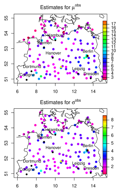
b

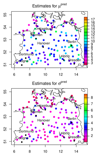
Figure 1: a Estimates $\hat{\mu}^{\rm obs}(l_{i})$ and $\hat{\sigma}^{\rm obs}(l_{i})$ for the location and scale parameters corresponding to the observed maximal wind speed at the stations in the northern part of Germany. b Estimates $\hat{\mu}^{\rm pred}(l_{i})$ and $\hat{\sigma}^{\rm pred}(l_{i})$ for the location and scale parameters corresponding to the forecasted maximal wind speed at the stations in the northern part of Germany.

As a fit of the GEV distribution to the forecast is needed for both verification of the marginal model and the bivariate Brown-Resnick model, we repeat our analysis replacing the observed maximal wind speed $v_{\max}^{\rm obs}(l_{i},d)$ by $v_{\max}^{\rm pred}(l_{i},d)$, i.e. a forecast for the maximal wind speed at station $l_{i}$ and day $d$. Here, we use the maximum over the 20 corresponding COSMO-DE ensemble members

$$v_{\max}^{\rm pred}(l_{i},d)=\max_{j=1,\ldots,20}v_{\max}^{(j)}(l_{i},d),\quad 1\leq i\leq 119,\ 1\leq d\leq 360,$$ (21)

which ensures that the distribution of $v_{\max}^{\rm pred}$ is close to a GEV distribution.

As the Kolmogorov-Smirnov test of the normalized estimates for $\xi^{\rm pred}$ yields a $p$-value of $0.53$ and the estimates differ significantly from the mean for seven stations (for three of them very significantly), we may assume a shape parameter of $\xi^{\rm pred}=\hat{\xi}^{\rm pred}=0.028$ at every station in Northern Germany. However, the hypotheses that the estimates for the location and the scale parameter follow a normal distribution have been both rejected. The maximum likelihood estimates $\hat{\mu}^{\rm pred}(l_{i})$ and $\hat{\sigma}^{\rm pred}(l_{i})$, $1\leq i\leq 119$, with fixed shape parameter are shown in Figure 1b. Here, the empirical correlation of the vectors of estimated location and scale parameters is just as strong as in case of the observations. Kolmogorov-Smirnov tests of the transformed data $x^{\rm pred}(l_{i},d)$ for every station yield $p$-values of at least 0.142 with and equal 0.748 in average which also indicates an appropriate fit.

The spatial dependence is modeled by a univariate Brown-Resnick process which is obtained by a weighted least squares fit of the extremal coefficient function. Here, the weights depend on the variance of the estimators $\hat{\vartheta}^{\rm obs}(l_{i},l_{j})$ (see Section 4) estimated by a jackknife procedure where the extremal coefficients are reestimated leaving out one month of data. The estimated extremal coefficients $\hat{\theta}^{\rm obs}$ and the fitted extremal coefficient function

$$\tilde{\theta}^{\rm obs}(s,t)=2\Phi\left(\sqrt{\gamma_{\hat{\vartheta}^{\rm obs}}(s-t)/2}\right),\quad s,t\in\mathbb{R}^{2}.$$

are displayed in Figure 2. Here, the estimated coefficients seem to be fitted quite well.

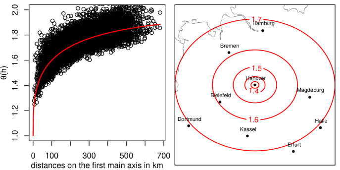
Figure 2: Left: The estimated extremal coefficients $\hat{\theta}^{\rm obs}$ (black circles) and the fitted extremal coefficient function $\tilde{\theta}^{\rm obs}$ (red line) of the normalized random field $X^{\rm obs}(\cdot,d)$ of observed wind gusts. Right: Contour level plot of the fitted extremal coefficient function $\tilde{\theta}^{\rm obs}(l_{0},\cdot)$ where $l_{0}$ is located at Hanover.

For verification, we first calculate the mean CRPS for each of the two models given by (16), ${\rm CRPS}^{{\rm obs}}(l_{i})$ and ${\rm CRPS}^{{\rm pred}}(l_{i})$, for every station $l_{i}$, $1\leq i\leq 119$. Then, the improvement or deterioration by using the GEV distributions of the observations instead of the forecasts is expressed in terms of the skill score (e.g., Gneiting and Raftery, 2007)

$$S(l_{i})=1-\frac{{\rm CRPS}^{{\rm obs}}(l_{i})}{{\rm CRPS}^{{\rm pred}}(l_{i})}$$

which has the value $1$ in case of an “optimal” model which equals $v_{\max}^{\rm obs}$ a.s. and the value 0 if both models yield the same result. Here, $S_{l_{i}}>0$ for $115$ of $119$ stations. For the skill score corresponding to the mean ${\rm CRPS}$ averaged over all the stations, we obtain

$$S=1-\frac{\sum_{i=1}^{119}{\rm CRPS}^{{\rm obs}}_{l_{i}}}{\sum_{i=1}^{119}{\rm CRPS}^{{\rm pred}}_{l_{i}}}\approx 0.293.$$

Note that, for simplicity, the reference model (16) for the predictions is based on the maximal ensemble members $v_{\max}^{\rm pred}(l_{i},d)$ only and further information given by the maximal wind speed forecasted by the other ensemble members are neglected. Thus, we further compare the CRPS of the GEV model for the observations, ${\rm CRPS}^{{\rm obs}}(l_{i})$, with the CRPS of the original COSMO-DE ensemble, ${\rm CRPS}^{{\rm orig}}(l_{i})$, taking the ensemble forecast as a probabilistic forecast with equal probability for each ensemble member. Here, the skill $\tilde{S}(l_{i})=1-\frac{{\rm CRPS}^{{\rm obs}}(l_{i})}{{\rm CRPS}^{{\rm orig}}(l_{i})}$ is positive for $37$ of $119$ only, with the skill of the averaged CRPS being $1-\frac{\sum_{i=1}^{119}{\rm CRPS}^{{\rm obs}}(l_{i})}{\sum_{i=1}^{119}{\rm CRPS}^{{\rm orig}}(l_{i})}\approx-0.032$. As the skill score is slightly negative, the COSMO-DE ensemble forecast seems to contain more information than our marginal model.

For the verification of the spatial model, for all pairs of locations $(l_{i},l_{j})$, $1\leq i<j\leq 119$, we estimate the energy scores $\widehat{ES}^{\rm BR}(l_{i},l_{j})$, based on $500$ samples of a Brown-Resnick process, and compare them with the estimated scores $\widehat{ES}^{\rm ind}(l_{i},l_{j})$ for the independence model, based on 50 samples of each GEV distribution. We obtain a positive skill score for $5819$ of $7002$ pairs of stations $(l_{i},l_{j})$ with a skill score of $0.025$ related to the mean energy score. Although this improvement by the univariate Brown-Resnick model compared to the independence model in terms of predictive skill seems negligible, realizations of gust fields look more realistic if spatial dependencies are respected.

Note that, for a fair comparison, we should avoid that training and validation of the model are based on the same data. Hence, we perform cross validation where the parameters are reestimated for every month, by leaving out the data for this month and using only the data for the other months for training. The GEV parameters estimated for different months in this way show very little variation corroborating the assumption that they are constant in time. Further, the verification results above are confirmed: We obtain skill scores of $0.285$ in the CRPS case compared with the GEV model for the forecast, $-0.048$ compared to the COSMO-DE ensemble and $0.035$ in case of the bivariate energy scores.

6.3 Applying the Bivariate Model

A bivariate Brown-Resnick process is fitted to the transformed data according to Section 4. The cross-variogram parameter estimate $\hat{\vartheta}$ leads to the fitted extremal coefficient function

$$\tilde{\theta}(l_{i},l_{j})={}\left(\tilde{\theta}^{k_{1},k_{2}}(l_{i},l_{j})\right)_{k_{1},k_{2}\in\{\text{``${\rm obs}$''},\text{``${\rm pred}$''}\}}={} 2\left(\Phi\Big{(}\sqrt{\gamma_{k_{1}k_{2}}(\hat{\vartheta};l_{i}-l_{j})/2}\Big{)}\right)_{k_{1},k_{2}\in\{\text{``${\rm obs}$''},\text{``${\rm pred}$''}\}}.$$

Figure 3 presents the estimated extremal coefficients $\hat{\theta}^{k_{1},k_{2}}(l_{i},l_{j})$, and the fitted extremal coefficient functions $\tilde{\theta}^{k_{1},k_{2}}(\cdot,\cdot)$ for $k_{1},k_{2}\in\{\text{``${\rm obs}$''},\text{``${\rm pred}$''}\}$. As illustrated, the fitted model seems to be appropriate with respect to the behavior of the extremal coefficient function. Figure 4 depicts a simulated realization of the corresponding Brown-Resnick process associated to the variogram $\gamma(\hat{\vartheta};\cdot)$ with standard Gumbel margins. The realization indicates a remarkable amount of positive correlation between $x^{\rm obs}$ and $x^{\rm pred}$ which emphasizes the gain of information by taking $x^{\rm pred}$ into account.

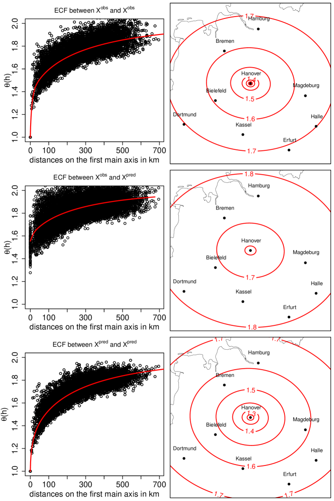
Figure 3: Left: The estimated extremal coefficients (black circles) and the fitted extremal coefficient function (red line) of the normalized bivariate random field $(X^{\rm obs},X^{\rm pred})$ of observed and forecasted wind gusts. Right: Contour level plots of the fitted extremal coefficient function $\tilde{\theta}(l_{0},\cdot)$ where $l_{0}$ is located at Hanover.

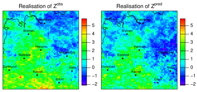
Figure 4: Simulated realization of a Brown-Resnick process associated to the variogram $\gamma(\vartheta;\cdot)$ with standard Gumbel margins.

In order to verify the bivariate model, we apply the post-processing procedure proposed in Subsection 5.1. However, due to the computational complexity of the conditional simulation, we do not simulate the observations at all stations simultaneously conditional on the forecast at all locations, but perform post-processing with sample size $K=100$ at each location separately conditioning on the forecast at the same location and two neighboring grid cells only. We calculate the CRPS of the post-processed distribution, ${\rm CRPS}^{\rm biv}(l_{i})$, and compare it with ${\rm CRPS}^{(NWP)}(l_{i})$, i.e. the CRPS belonging to the empirical distribution of the original COSMO-DE ensemble, yielding a positive skill score for $103$ of $119$ stations where the skill score related to the mean CRPS equals $0.164$ ($0.148$ cross-validated). Thus, we may conclude that the post-processing procedure based on the bivariate Brown-Resnick model is able to improve the forecast given by COSMO-DE ensemble.

Appendix: Proof of Theorem 1

For $i,j\in\{1,2\}$, and $h\in\mathbb{R}^{D}$, we obtain

$$\left(\sqrt{\gamma_{ii}(h)}-\sqrt{\gamma_{jj}(h)}\right)^{2}{}={}\gamma_{ii}(h)-2\sqrt{\gamma_{ii}(h)\gamma_{jj}(h)}+\gamma_{jj}(h)$$

$$\leq{} \gamma_{ii}(h)-\operatorname{Cov}(W^{(i)}(h)-W^{(i)}(0),W^{(j)}(h)-W^{(j)}(0))+\gamma_{jj}(h)$$

$$={} \frac{1}{2}\operatorname{Var}\left(W^{(i)}(h)-W^{(i)}(0)-W^{(j)}(h)+W^{(j)}(0)\right)$$

$$={} \gamma_{ij}(0)-\operatorname{Cov}\left(W^{(i)}(h)-W^{(j)}(h),W^{(i)}(0)-W^{(j)}(0)\right)+\gamma_{ij}(0){}\leq{}4\gamma_{ij}(0),$$

where we used the Cauchy-Schwarz inequality for both inequalities. Analogously, we get the assessment

$$\left(\sqrt{\gamma_{ii}(h)}-\sqrt{\gamma_{ji}(h)}\right)^{2}{}={}\gamma_{ii}(h)-2\sqrt{\gamma_{ii}(h)\gamma_{ji}(h)}+\gamma_{ji}(h)$$

$$\leq{} \gamma_{ii}(h)-\operatorname{Cov}(W^{(i)}(h)-W^{(i)}(0),W^{(j)}(h)-W^{(i)}(0))+\gamma_{ji}(h)$$

$$={} \frac{1}{2}\operatorname{Var}\left(W^{(i)}(h)-W^{(j)}(h)\right){}={}\gamma_{ij}(0).$$

Thus, the assertion of the theorem follows with $\gamma_{0}=\gamma_{11}$.

References

- Baldauf et al. (2011) Baldauf, M., A. Seifert, J. Förstner, D. Majewski, M. Raschendorfer, and T. Reinhardt (2011). Operational convective-scale numerical weather prediction with the COSMO model. Mon. Wea. Rev. 139, 3887–3905.
- Berg et al. (1984) Berg, C., J. P. R. Christensen, and P. Ressel (1984). Harmonic Analysis on Semigroups: Theory of Positive Definite and Related Functions. New York: Springer.
- Brasseur (2001) Brasseur, O. (2001). Development and application of a physical approach to estimating wind gusts. Mon. Wea. Rev. 129(1), 5–25.
- Brown and Resnick (1977) Brown, B. M. and S. I. Resnick (1977). Extreme values of independent stochastic processes. J. Appl. Probab. 14(4), 732–739.
- Chilès and Delfiner (2012) Chilès, J.-P. and P. Delfiner (2012). Geostatistics. Modeling Spatial Uncertainty (Second ed.). Hoboken, NJ: Wiley.
- Clark et al. (1989) Clark, I., K. L. Basinger, and W. V. Harper (1989). MUCK-a novel approach to co-kriging. In Geostatistical, sensitivity, and uncertainty methods for ground-water flow and radionuclide transport modeling., San Francisco. Battelle Memorial Institute.
- Coles (1993) Coles, S. (1993). Regional modelling of extreme storms via max-stable processes. J. R. Statist. Soc., Ser. B. 55, 797–816.
- Coles (2001) Coles, S. (2001). An Introduction to Statistical Modeling of Extreme Values. London: Springer.
- Coles and Tawn (1996) Coles, S. and J. Tawn (1996). Modelling extremes of the areal rainfall process. J. R. Statist. Soc., Ser. B 58, 329–347.
- Conradsen et al. (1984) Conradsen, K., L. B. Nielsen, and L. P. Prahm (1984). Review of Weibull statistics for estimation of wind speed distributions. J. Clim. Appl. Meteorol. 23, 1173–1183.
- Cooley et al. (2006) Cooley, D., P. Naveau, and P. Poncet (2006). Variograms for spatial max-stable random fields. In Dependence in Probability and Statistics, pp. 373–390. New York: Springer.
- Dombry et al. (2013) Dombry, C., F. Éyi-Minko, and M. Ribatet (2013). Conditional simulation of max-stable processes. Biometrika 100(1), 111–124.
- Engelke et al. (2015) Engelke, S., A. Malinowski, Z. Kabluchko, and M. Schlather (2015). Estimation of Hüsler–Reiss distributions and Brown–Resnick processes. J. R. Statist. Soc., Ser. B 77(1), 239–265.
- Friederichs and Thorarinsdottir (2012) Friederichs, P. and T. L. Thorarinsdottir (2012). Forecast verification for extreme value distributions with an application to probabilistic peak wind prediction. Environmetrics 23(7), 579–594.
- Gebhardt et al. (2011) Gebhardt, C., S. Theis, M. Paulat, and Z. Ben Bouallègue (2011). Uncertainties in COSMO-DE precipitation forecasts introduced by model perturbations and variation of lateral boundaries. Atmos. Res. 100(2), 168–177.
- Gelfand et al. (2010) Gelfand, A. E., P. Diggle, P. Guttorp, and M. Fuentes (2010). Handbook of Spatial Statistics. Boca Raton: CRC Press.
- Genton et al. (2015) Genton, M. G., S. A. Padoan, and H. Sang (2015). Multivariate max-stable spatial processes. Biometrika 102(1), 215–230.
- Gneiting et al. (2010) Gneiting, T., W. Kleiber, and M. Schlather (2010). Matérn cross-covariance functions for multivariate random fields. J. Amer. Statist. Assoc. 105(491), 1167–1177.
- Gneiting and Raftery (2007) Gneiting, T. and A. E. Raftery (2007). Strictly proper scoring rules, prediction, and estimation. J. Amer. Statist. Assoc. 102(477), 359–378.
- Guttorp and Gneiting (2006) Guttorp, P. and T. Gneiting (2006). Studies in the history of probability and statistics xlix on the matern correlation family. Biometrika 93(4), 989–995.
- Huser and Davison (2014) Huser, R. and A. C. Davison (2014). Space-time modelling of extreme events. J. R. Statist. Soc., Ser. B 76(2), 439–461.
- Kabluchko (2011) Kabluchko, Z. (2011). Extremes of independent Gaussian processes. Extremes 14(3), 285–310.
- Kabluchko et al. (2009) Kabluchko, Z., M. Schlather, and L. de Haan (2009). Stationary max-stable fields associated to negative definite functions. Ann. Probab. 37(5), 2042–2065.
- Leadbetter et al. (1983) Leadbetter, M. R., G. Lindgren, and H. Rootzén (1983). Extremes and Related Properties of Random Sequences and Processes. New York: Springer.
- Molchanov and Stucki (2013) Molchanov, I. and K. Stucki (2013). Stationarity of multivariate particle systems. Stochastic Process. Appl. 123(6), 2272–2285.
- Papritz et al. (1993) Papritz, A., H. Künsch, and R. Webster (1993). On the pseudo cross-variogram. Math. Geol. 25(8), 1015–1026.
- Pavia and O’Brien (1986) Pavia, E. G. and J. J. O’Brien (1986). Weibull statistics of wind speed over the ocean. J. Clim. Appl. Meteorol. 25, 1324–1332.
- Peralta et al. (2012) Peralta, C., Z. Ben Bouallégue, S. E. Theis, C. Gebhardt, and M. Buchhold (2012). Accounting for initial condition uncertainties in COSMO-DE-EPS. J. Geophys. Res. 117, D07108.
- Ribatet (2013) Ribatet, M. (2013). Spatial extremes: Max-stable processes at work. J. Soc. Fr. Stat. 154(2), 156–177.
- Schilling et al. (2010) Schilling, R. L., R. Song, and Z. Vondraček (2010). Bernstein Functions: Theory and Applications. Berlin: Gruyter.
- Schlather and Tawn (2003) Schlather, M. and J. A. Tawn (2003). A dependence measure for multivariate and spatial extreme values: Properties and inference. Biometrika 90(1), 139–156.
- Sloughter et al. (2007) Sloughter, J. M. L., A. E. Raftery, T. Gneiting, and C. Fraley (2007). Probabilistic quantitative precipitation forecasting using bayesian model averaging. Mon. Wea. Rev. 135, 3209–3220.
- Smith (1985) Smith, R. L. (1985). Maximum likelihood estimation in a class of nonregular cases. Biometrika 72(1), 67–90.
- Smith (1990) Smith, R. L. (1990). Max–stable processes and spatial extremes. Unpublished manuscript.
- Stein (1999) Stein, M. L. (1999). Interpolation of Spatial Data: Some Theory for Kriging. Springer Series in Statistics. New York: Springer.