Density anomaly of charged hard spheres of different diameters in a mixture with core-softened model solvent. Monte Carlo simulation results

Abstract

Very recently the effect of equisized charged hard sphere solutes in a mixture with core-softened fluid model on the structural and thermodynamic anomalies of the system has been explored in detail by using Monte Carlo simulations and integral equations theory [J. Chem. Phys., 2012, 137, 244502]. Our objective of the present short work is to complement this study by considering univalent ions of unequal diameters in a mixture with the same soft-core fluid model. Specifically, we are interested in the analysis of changes of the temperature of maximum density (TMD) lines with ion concentration for three model salt solutes, namely sodium chloride, potassium chloride and rubidium chloride models. We resort to Monte Carlo simulations for this purpose. Our discussion also involves the dependences of the pair contribution to excess entropy and of constant volume heat capacity on the temperature of maximum density line. Some examples of the microscopic structure of mixtures in question in terms of pair distribution functions are given in addition.

Key words: liquid theory, soft-core model fluid, electrolyte solution, canonical Monte Carlo simulations, density anomaly

PACS: 61.20.-p, 61.20.Gy, 6120.Ja, 61.20.Ne, 61.20.Qg, 65.20.-w

Abstract

Недавно було дослiджено вплив заряджених твердих сфер однакового розмiру як розчиненої речовини на структурнi i термодинамiчнi аномалiї системи, в якiй застосовано модель плину з потенцiалом з м’яким кором як розчинник. Застосовувався метод моделювання Монте Карло та теорiя iнтегральних рiвнянь [J. Chem. Phys., 2012, 137, 244502]. Метою даної роботи є доповнити попереднє дослiдження, розглядаючи одновалентнi iони з рiзними дiаметрами у сумiшi з таким самим модельним розчинником. Зокрема, нас цiкавить аналiз змiн температури максимальної густини при збiльшеннi концентрацiї iонiв для трьох модельних солей, хлористого натрiю, хлористого калiю i хлористого рубiдiю. З цiєю метою застосовуємо моделювання Монте Карло. Наше обговорення також включає залежнiсть парного внеску до надлишкової ентропiї та теплоємностi при сталому об’ємi вздовж лiнiї температури максимальної густини. Деякi приклади мiкроскопiчної структури у виглядi парних функцiй розподiлу приведено на додаток.

Ключовi слова: теорiя рiдин, модель плину з м’яким кором, розчин електролiту, моделювання методом канонiчного Монте Карло, аномалiя густини

1 Introduction

It is our honor and pleasure to make contribution to this special issue dedicated to brilliant scientist Prof. Myroslav Holovko on the occasion of his 70th birthday. During last years we were influenced by his developments and profound results along different lines of research in the theory of liquids and mixtures, interfacial phenomena and phase transitions. We appreciate his mentorship in some projects, many useful pieces of advice and friendly discussions concerning topics of our common interest. During many years Myroslav Holovko explored electrolyte solutions in very detail, see e.g., the classical monograph [1] written by him together with his teacher Prof. I. Yukhnovskyi that summarizes their effort prior to 1980. Later results can be found in many articles and reviews.

The principal objective of the present work is to complete one extension of our very recent study of solutions comprising solute ions and a soft-core model fluid as a solvent [2]. During last decade many studies in the theory of fluids have been focused on single-component, isotropic core-softened models in which the repulsive part of the interparticle interaction potential is peculiar (‘‘softer’’) at ‘‘intermediate’’ interparticle separations while a hard-core repulsion acts at short distances. This region of peculiar dependence of the pair interparticle interaction is often described by linear or nonlinear ramp [3, 4, 5, 6, 7, 8], by a shoulder [9, 10] or Gaussian term [11, 12, 13], or another more sophisticated functional dependence, see e.g., recent review [14] and references therein. A more complete list of references has been given in [2] as well.

Unfortunately, the complex shape of the interaction in this type of models requires application of solely numerical procedures for their solution. However, peculiar structural, thermodynamic and dynamic properties relevant to certain real liquids can be reached. Models of single-component fluids with isotropic core-softened potential have been studied by computer simulations in numerous works, see the list of references in [2]. For purposes of the present work it is necessary to mention that the fluids with spherically symmetric core-softened potentials exhibit anomalies in thermodynamic and dynamic properties in close similarity to those observed in liquids with directional inter-particle interactions, such as water, silica, phosphorous, and some liquid metals. One of the examples of such anomalous behavior is the presence of the fluid density maximum as a function of temperature. Moreover, some of the soft-core fluid models exhibit puzzling liquid-liquid coexistence envelope terminating at the critical point, in addition to common liquid-vapor phase transition. Thermodynamic and other anomalies can be related to this additional phase transition, see e.g., references [15, 16, 17]. The soft-core models by design miss the orientational interparticle correlations. Thus, their correspondence to, for example, water or aqueous solutions is restricted to thermodynamic properties. Nevertheless, the soft-core models are simple and permit to capture the peculiarities of thermodynamic properties quite adequately [14].

Theoretical studies of solutions in which a model solvent exhibits thermodynamic properties with anomalies have been attempted recently by different authors, see e.g., [18, 19, 20, 21, 22, 23, 24]. Several important particular issues were explored, namely the solubility of apolar solutes in such solvents, the effect of solute species on the temperature of maximum density line, on heat capacity extrema and others. On the other hand, following our previous theoretical and simulation developments [25, 26], we applied similar modelling, but involved ionic solutes rather than nonpolar species [2]. We examined the effect of ionic solutes on the microscopic structure and thermodynamics of solutions with a soft-core solvent that possesses anomalies in one-phase region. Experiments [27, 28, 29, 30] and computer simulations [31, 32, 33] have shown that certain anomalies of thermodynamic properties are preserved in ionic aqueous solutions for low and up to moderate ion concentrations. They become weaker and finally disappear, if the concentration of ions increases but remains below the solubility limit.

In contrast to the initial stage of this project [2], we consider a mixture of singly charged cations and anions modelled as charged hard spheres and solvent particles described by a soft-core model, all of them having nonequal diameters. The system is studied by the canonical Monte Carlo simulations. The following discussion of the model and methods is brief in order to avoid unnecessary repetitions of [2], only the essential elements are given to benefit the reader.

2 Model and method

The system in question consists of ionic solute (salt) and solvent. The ionic subsystem is a mixture of positively and negatively charged hard spheres with arbitrary diameters, $\sigma_{+}$ and $\sigma_{-}$, the charge is located at the particle center. Ions and solvent particles are immersed in a dielectric background characterized by dielectric constant $\varepsilon$. The interaction potential between ions $i$ and $j$ is,

$$U_{ij}(r)=\left\{\begin{array}[]{ll}\infty\,,&\hbox{$r<(\sigma_{i}+\sigma_{j})/2$},\\ \displaystyle\frac{e^{2}z_{i}z_{j}}{4\pi\varepsilon_{0}\varepsilon r}\,,&\hbox{$r\geqslant(\sigma_{i}+\sigma_{j})/2$},\end{array}\right.$$ (3)

where $e$ is the elementary charge, $z_{i}=|z_{-}|=1$ are the valencies of ions, $\varepsilon_{0}$ is the permittivity of free space, and $r$ is the inter-particle distance. As in [2], we use the core-softened model by Barros de Oliveira et al. [11, 12, 13] that possesses thermodynamic, structural, and dynamic anomalies. The potential is a sum of the Lennard-Jones and a Gaussian terms,

$$U_{\mathrm{ss}}(r)=4\varepsilon_{\mathrm{ss}}\left[\left(\frac{\sigma_{\mathrm{s}}}{r}\right)^{12}-\left(\frac{\sigma_{\mathrm{s}}}{r}\right)^{6}\right]+a\varepsilon_{\mathrm{s}}\exp\left[-\frac{1}{c^{2}}\left(\frac{r-r_{0}}{\sigma_{\mathrm{s}}}\right)^{2}\right],$$ (4)

with $\varepsilon_{\mathrm{ss}}$ — the solvent-solvent interaction energy and $\sigma_{\mathrm{s}}$ — the diameter of a solvent particle. Parameters $a$, $c$, and $r_{0}$ are taken as in the original work [11] ($a=5$, $c=1$, and $r_{0}/\sigma_{\mathrm{s}}=0.7$). With this choice of parameters, the inter-particle attraction is strongly depressed and thus there is no liquid-gas transition in the solvent subsystem [34].

The pressure-temperature curves calculated for the pure solvent at certain densities have a minimum (i.e., $(\partial P/\partial T)_{\rho}=0$) and consequently $(\partial\rho/\partial T)_{P}$ vanishes for some thermodynamic states. The region of density anomaly corresponds to the state points for which $(\partial\rho/\partial T)_{P}>0$ and is bounded by the locus of points for which the thermal expansion coefficient equals zero.

There is some room for the choice of ion-solvent interaction. However, to be consistent with our previous work [2], the interaction between an ion ($i$), and a solvent ($s$) particle is taken simply in the form of Lennard-Jones (12-6) potential,

$$U_{\mathrm{is}}(r)=4\varepsilon_{\mathrm{is}}\left[\left(\frac{\sigma_{\mathrm{is}}}{r}\right)^{12}-\left(\frac{\sigma_{\mathrm{is}}}{r}\right)^{6}\right],$$ (5)

where $\varepsilon_{\mathrm{is}}$ is the ion-solvent interaction energy and $\sigma_{\mathrm{is}}=(\sigma_{\mathrm{i}}+\sigma_{\mathrm{s}})/2$. The reduced temperature for the solvent subsystem is defined as $T^{*}=k_{\mathrm{B}}T/\varepsilon_{\mathrm{s}}$, where $k_{\mathrm{B}}$ is the Boltzmann constant and $T$ is the absolute temperature.

In order to describe the energetic aspects of interactions between all species, it is necessary to define the parameter $\alpha=T^{*}/T^{*}_{\mathrm{el}}$ as the ratio between the reduced temperature for the solvent subsystem ($T^{*}$), and the reduced temperature of the ionic subsystem, $T^{*}_{\mathrm{el}}=\sigma_{-}/\lambda_{\mathrm{B}}$, where $\lambda_{\mathrm{B}}=e^{2}/(4\pi\varepsilon_{0}\varepsilon k_{\mathrm{B}}T)$ is the Bjerrum length, $\lambda_{\mathrm{B}}=7.14$ Å. Similar to the previous study [2], we choose $\alpha=0.25$. Thus, if the solvent is even at a rather low temperature, the ionic system remains far from the possible vapor – liquid type criticality. The mixing rule for ion-solvent potential is applied such that: $\varepsilon_{\mathrm{is}}=(\varepsilon_{ii}\varepsilon_{jj})^{1/2}$, where $\varepsilon_{\mathrm{ss}}=1/T^{*}$, $\varepsilon_{--}=1/T^{*}_{\mathrm{el}}$ and $\varepsilon_{++}=(\sigma_{-}/\sigma_{+})/T^{*}_{\mathrm{el}}$.

We performed Monte Carlo computer simulations in the canonical ensemble and in the cubic simulation box according to common algorithms [35, 36]. The simulation was started from a configuration of randomly distributed particles. The number of ions in the box, $N_{\mathrm{ion}}$ ($N_{\mathrm{ion}}=N_{+}+N_{-}$) was chosen to provide their reasonable statistics and along with the desired ion concentration, $x_{\mathrm{ion}}$ [$x_{\mathrm{ion}}=N_{\mathrm{ion}}/(N_{\mathrm{ion}}+N_{\mathrm{s}})$], where $N_{\mathrm{s}}$ is the number of solvent particles resulting from $N_{\mathrm{ion}}$ and $x_{\mathrm{ion}}$. In addition, we picked up the desired total dimensionless density of the system, $\rho^{*}$, $\rho^{*}=(N_{+}\sigma_{+}^{3}+N_{-}\sigma_{-}^{3}+N_{\mathrm{s}}\sigma_{s}^{3})/L^{3}$, where $L$ is the length of the box edge resulting from previously given parameters. Coulomb interactions were taken into account by using the Ewald summation  [35, 36] with 337 wave vectors and the inverse length equal to $5/L$).

In this work, we explore three model salts in the soft-core solvent, namely the NaCl ($\sigma_{+}=2.21$ Å, $\sigma_{-}=4.42$ Å), KCl ($\sigma_{+}=4.74$ Å, $\sigma_{-}=4.42$ Å) and RbCl ($\sigma_{+}=5.27$ Å, $\sigma_{-}=4.42$ Å) see e.g., [37, 38]. In all cases, we assume $\sigma_{\mathrm{s}}=3.166$ Å in close similarity to the SPCE model of water. Each of the systems was first equilibrated over $10^{8}$ attempted configurations followed by a series of production runs of at least $5\times 10^{7}$ attempted particle displacements to obtain the relevant average properties of the system under investigation (excess internal energy, compressibility factor, heat capacity at constant volume, pair excess entropy, and radial distribution functions). The number of ions present in the simulation box was in the range between $150$ and $400$ (dependent on the desired density). The excess internal energy of the system was obtained directly as an ensemble average. The equation of state was calculated by [39]

$$\frac{PV}{Nk_{\mathrm{B}}T}=1-\frac{1}{3N}\left\langle r\frac{\partial\beta U_{\mathrm{tot}}}{\partial r}\right\rangle+\frac{2\pi}{3}\sum_{i}\sum_{j}x_{i}\frac{N_{j}}{V}\sigma_{ij}^{3}g_{ij}(\sigma_{ij})\,,\qquad(i,j=+,-),$$ (6)

where $U_{\mathrm{tot}}$ is the total excess internal energy of the system and $g_{ij}(\sigma_{ij})$ is the contact value of the appropriate ion-ion radial distribution function. Pair excess entropy was determined from the expression [40]

$$\frac{S_{2,\mathrm{ex}}}{k_{\mathrm{B}}}=-2\pi\rho\sum_{i,i}x_{i}x_{j}\int\left[g_{ij}(r)\ln g_{ij}(r)-g_{ij}(r)+1\right]r^{2}{\mathrm{d}}r\,,$$ (7)

where $x_{i}$ is the number fraction of species $i$, and $g_{ij}(r)$ are the pair distribution functions of species $i$ and $j$. The heat capacity at constant volume was determined from the energy fluctuations as

$$C_{V}=\left(\langle U_{\mathrm{tot}}^{2}\rangle-\langle U_{\mathrm{tot}}\rangle^{2}\right)/k_{\mathrm{B}}T^{2}\,.$$ (8)

3 Results and discussion

     

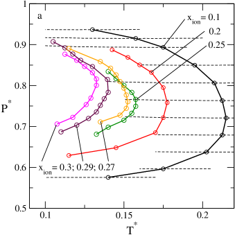
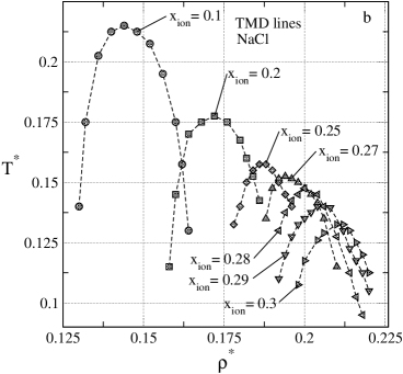
Figure 1: (Color online) Temperature of maximum density lines of the NaCl model in the $P^{*}-T^{*}$ plane (panel a) $T^{*}-\rho^{*}$ plane (panel b).

     

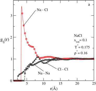
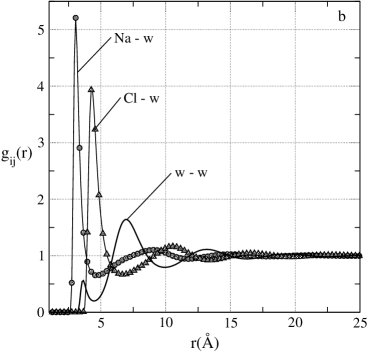
Figure 2: (Color online) Pair distribution functions of the NaCl model. Parameters of the system are given in the figure.

     

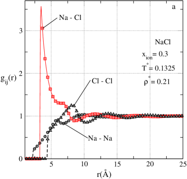
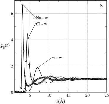
Figure 3: (Color online) Pair distribution functions of the NaCl model. Parameters of the system are given in the figure.

     

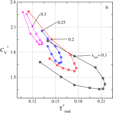
Figure 4: (Color online) The behavior of the pair contribution to excess entropy (panel a) and of reduced heat capacity (panel b) on the temperature of maximum density of the NaCl model at different concentration of ions.

First series of our calculations concern the NaCl salt model ($\sigma_{+}=2.21$ Å, $\sigma_{-}=4.42$ Å) in the soft-core solvent. The cation is rather small and its diameter is smaller compared to the anion and to the diameter of solvent particles. The results for $P^{*}$ ($P^{*}=P\sigma^{3}_{\mathrm{s}}/\varepsilon_{\mathrm{s}}$) as a function of $T^{*}$ for a set of densities of the mixture at fixed ion concentration $x_{\mathrm{ion}}=0.1$ are given by short-dashed lines in figure 1 (a). Each line has a minimum (it is difficult to see it on the scale of such combined figure) marked by a circle. By joining the circles, one can construct the temperature of maximum density line at this particular ion concentration, $x_{\mathrm{ion}}=0.1$. The $P^{*}(T^{*})$ lines at a given $\rho^{*}$ are built by joining points obtained as an average from several runs. Actually, it is quite a tedious procedure. We perform a series of calculations to construct the TMD lines for different $x_{\mathrm{ion}}$, up to $x_{\mathrm{ion}}=0.3$. Each of the lines has an extremal point that shifts to a higher pressure and lower temperature with an increasing $x_{\mathrm{ion}}$. Moreover, the TMD lines shrink with an increasing ion concentration. These trends were already discussed by us for the model in which all the species involved are of equal diameter [2]. Slightly different view on the changes of the TMD lines is given in figure 1 (b). The shift of the TMD lines to higher $\rho^{*}$ with a growing $x_{\mathrm{ion}}$ can be explained by augmenting the excluded volume effects in the system, if ions are added to the solvent. On the other hand, the extremum point of the TMD along the temperature axis goes down due to the overall growth of attraction, principally between oppositely charged ions.

Previously, we discussed the evolution of the microscopic structure of the model characterized by equal diameters of all species on the density at a fixed $T^{*}$ and $x_{\mathrm{ion}}$, see figures 1 and 2 of [2]. Trends of behavior of the pair distribution functions are similar to the model with non-equal diameters. Two examples of the distribution of particles at thermodynamic states on the relevant TMD line are given here in figures 2 and 3. In the case of a lower density and lower ion concentration (figure 2), we can attribute the shape of the ion-ion distribution functions to the formation of Na–S–Cl, Cl–S–Cl and Na–S–Na structures or complexes, i.e., of ions separated by a single solvent molecule, corresponding to the local maxima at $(\sigma_{\mathrm{Na}}+\sigma_{\mathrm{Cl}})/2+w_{1}$, $\sigma_{\mathrm{Cl}}+w_{1}$ and $\sigma_{\mathrm{Na}}/2+w_{1}$ distances, respectively. Here, $w_{1}$ is the distance corresponding to the first maximum of the distribution of solvent species, $g_{ww}(r)$ at 3.63 Å, approximately. Similarly, one can observe trends of formation of clusters at a distance $(\sigma_{\mathrm{Na}}+\sigma_{\mathrm{Cl}})/2+w_{2}$, where $w_{2}$ is the distance corresponding to the position of the principal maximum of the distribution of solvent species at 7 Å, approximately. Due to a stronger repulsion between small cations, the formation of Na–S–Na structure is less favorable compared to Cl–S–Cl structure at these conditions.

On the other hand, if one considers the model at $x_{\mathrm{ion}}=0.3$ at a point of the TMD line with slightly higher total density but substantially lower temperature (figure 3) compared to the case described in figure 2, the inter-ion electrostatic correlations are expected to be stronger. Nevertheless, screening of interactions between ions is expected to be more pronounced. Under the conditions given in figure 3, one can see that the contact value of $g_{\mathrm{NaCl}}(r)$ is practically of the same order as in figure 2. However, the height of the shoulder of this function at $r\approx 6.9$ Å describing the correlation between oppositely charged ions separated by a single solvent particle is lower than in figure 2. On the other hand, the height of the first maximum of $g_{\mathrm{ClCl}}$ is higher as an evidence of weaker repulsion between equally charged anions. Possible formation of Na–$w_{1}$–Na is also more pronounced, cf. figure 2. The cation-solvent correlations are enhanced in the present case (at this low temperature) compared to anion-solvent correlation and compared to the case discussed in figure 2.

We now again return to thermodynamic manifestations of the existence of the TMD lines. A quantitative cumulative measure of the distribution of particles of different species is commonly given in terms of the pair contribution to the excess internal energy per particle as a function of the total density for different compositions of the mixture and at different reduced temperatures. In previous studies of the single-component soft-core model fluids it was suggested that the relation between the density and diffusion anomalies and the microscopic structure of the system can be explored in terms of the excess-entropy-based framework, see e.g., [41]. It has been shown that the presence of the density and the diffusion anomalies is related to the effect of excess entropy on the fluid density. Our discussion concerns $S_{2,\mathrm{ex}}$ defined for a mixture by equation (7).

However, in contrast to previous works, we have calculated the dependence of $S_{2,\mathrm{ex}}$ as a function of the temperature of maximum density rather than the total density of the model. In this respect, our results given in figure 4 (a) correspond to the TMD lines presented in figure 1. For example, the left hand part of the TMD line for $x_{\mathrm{ion}}=0.1$ in figure 1 (b) that is characterized by $\mathrm{d}T^{*}/\mathrm{d}\rho^{*}>0$ corresponds to the upper part (lower absolute values) of the corresponding line for $S_{2,\mathrm{ex}}$ on $T^{*}_{\mathrm{tmd}}$. What can we learn from these functions? First observation is that the $S_{2,\mathrm{ex}}(T^{*}_{\mathrm{tmd}})$ curves shift to lower values of $S_{2,\mathrm{ex}}$ and lower values for $T^{*}_{\mathrm{tmd}}$ with an increasing concentration of ionic solutes. Moreover, these curves shrink with increasing ion concentration. At low values of $x_{\mathrm{ion}}$ (and at vanishing $x_{\mathrm{ion}}$ as well) the curve $S_{2,\mathrm{ex}}(T^{*}_{\mathrm{tmd}})$ has a maximum such that $\mathrm{d}S_{2,\mathrm{ex}}/\mathrm{d}(T^{*}_{\mathrm{tmd}})<0$ in the small region of $T^{*}_{\mathrm{tmd}}$ after the point $\mathrm{d}S_{2,\mathrm{ex}}/\mathrm{d}(T^{*}_{\mathrm{tmd}})=0$. This point does not coincide with the maximum temperature of the TMD line. Discontinuity of this derivative is expected, however, around the point at which $T^{*}_{\mathrm{tmd}}$ reaches its maximum. This behavior is much less pronounced at high values for ion concentration in a mixture. The existence of such type of peculiar behavior seems to be worth to investigate in more detail for other soft-core solvent models and for say nonpolar solutes in various solvents for the sake of comparison with the case of ionic solutes.

A rather similar discussion can be presented while considering the dependence of the reduced constant volume heat capacity, $C^{*}_{V}$ on $T^{*}_{\mathrm{tmd}}$, figure 4 (b) [$C^{*}_{V}=C_{V}/(N_{\mathrm{ion}}+N_{\mathrm{s}})k_{\mathrm{B}}$]. The heat capacity was ‘‘measured’’ in simulations through the fluctuations of internal energy according to equation (8). It is quite difficult to evaluate the heat capacity precisely due to fluctuations, especially at low temperatures. One way to suppress the fluctuations of the $C^{*}_{V}$ values is to consider bigger boxes with a bigger number of particles, but then the simulations become quite lengthy in time. Shift and shrinking of the $C^{*}_{V}(T^{*}_{\mathrm{tmd}})$ curves with an increasing ion concentration are well pronounced. However, the behavior of $C^{*}_{V}(T^{*}_{\mathrm{tmd}})$ around the extremum point of the TMD line must be studied in more detail.

     

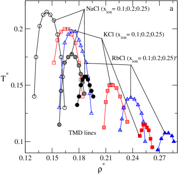
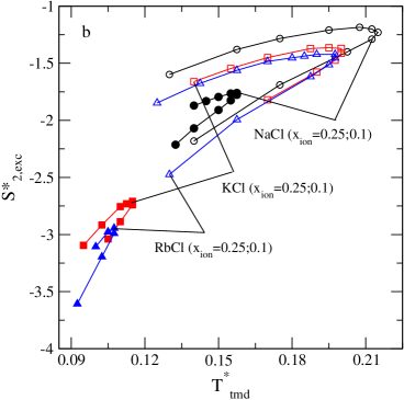
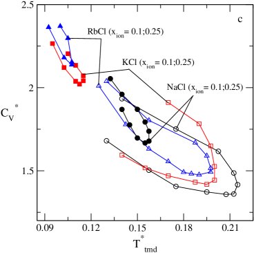
Figure 5: (Color online) Temperature of maximum density lines of the NaCl, KCl and RbCl ion models with the soft-core solvent in the $T^{*}-\rho^{*}$ plane at different concentration of ions (panel a). The behavior of the pair contribution to excess entropy (panel b) and of reduced heat capacity (panel c) on the temperature of maximum density of the NaCl, KCl and RbCl models at different concentration of ions.

After rather comprehensively examining the properties of the TMD lines of the model NaCl salt in the soft-core solvent in question at different ion concentrations, we would like to proceed to the results obtained for other two salts with bigger cations, namely the KCl and RbCl. The assumed diameters of cations were mentioned in the previous section, but we repeat the numbers for the sake of convenience of the reader KCl ($\sigma_{+}=4.74$ Å) and RbCl ($\sigma_{+}=5.27$ Å). In the former case, the diameter of cation does not differ much from the diameter of the anion $\sigma_{\mathrm{Cl}}=4.42$ Å. From the analysis of the $T^{*}-\rho^{*}$ projections of the TMD lines given in figure 5 (a), we would like to conclude that in the present formulation of the interactions in the model, the principal factor determining the location of the TMD lines seems to be the excluded volume effects. Namely, at $x_{\mathrm{ion}}=0.1$, the difference between TMD lines is reasonably big, if one changes from NaCl salt to KCl salt. The difference between KCl and RbCl cases is small as expected, because the cation diameter does not change much. It seems that the shift of the TMD line to higher densities is determined by the amount of excluded volume added to the system. On the other hand, the enhanced excluded volume effects also lead to a lower extremal point along the temperature axis of the TMD lines. However, this shift of TMD lines on temperature axis is to a great extent effected by the electrostatic interactions between ions. If the ion concentration increases for each salt model, the lines substantially shift to lower temperatures. Unfortunately, the solvent in question (due to a set of parameters assumed) does not exhibit vapor – liquid criticality. Therefore, we do not have a natural lower boundary for the TMD lines in, for example, the $T^{*}-\rho^{*}$ projection. Our preliminary calculations have shown that quite short TMD lines still exist for $x_{\mathrm{ion}}=0.31$ and for 0.32 for NaCl model. The shifts of the TMD lines along the density and temperature axes given in figure 5 (a) are also reflected by the behavior of excess pair entropy and of the reduced heat capacity, see figures 5 (b) and 5 (c), respectively. Shrinking of these curves with an increasing ion concentration is quite evident. Trends of the behavior of $S^{*}_{2,\mathrm{exc}}$ and of $C^{*}_{V}$ are similar to those discussed for the model NaCl salt in the soft-core solvent just above.

To conclude, in the present short communication we considered one extension of our very recent work [2] concerning a simple model mixture of ions and soft-core solvent fluid by using Monte Carlo computer simulations. Our extension consists in considering ions of non-equal diameters and different from the diameter of solvent particles. We were interested to study how the presence of ion solutes affects thermodynamic properties of the system compared to the single-component fluid, specifically the temperature of maximum density line. For this purpose, we studied three model solute salts, namely the model for NaCl, KCl and RbCl. Our results confirm that the mixtures based on a soft-core solvent in question preserve this anomalous behavior at $x_{\mathrm{ion}}=0.1$ 0.2, 0.25, and 0.3, if the cation is small, e.g., for NaCl model. However, for the model with a big cation, e.g., RbCl the density anomaly disappears at $x_{\mathrm{ion}}$ around 0.27.

The TMD lines were constructed from the simulation data for a set of isochores. They shift to lower temperatures and higher densities with an increasing ion concentration in the $T^{*}-\rho^{*}$ plane. The TMD line shrinks and moves to lower values of the reduced temperature with an increasing ion concentration for each model salt. These observations agree with the results of molecular dynamics simulations [32] for much more elaborate model for aqueous solutions. We have seemingly made interesting observations about the dependence of the excess pair entropy and constant volume heat capacity along the TMD line at different ion concentrations. Still it is necessary to complement our study by simulations of uncharged solutes with different characteristics mixed with applied or another soft-core model for the solvent subsystem. It is known that in the presence of uncharged, non-polar solutes, the curves describing the anomalies shift as well, see e.g. [18]. However, for example, the TMD line changes essentially depend on the solute concentration and strength of solute-solvent interactions. In order to compare our present observations with the models of uncharged solutes in soft-core solvents, additional simulations are necessary. This project is in progress in our laboratory at present. Intuitively, one should expect the most pronounced differences between the effects of ions and non-polar solutes if the ion concentration is low or, in other words, when the screening of ion-ion interaction is not well pronounced.

There remains much room for extensions of the present work. In order to validate the results concerning the trends for anomalies with increasing ion concentrations, it is worth to extend the calculations and establish the solubility limits. It is necessary to explore how the modification of the cross solute-solvent interaction potentials would affect the TMD lines. Another important issue is to investigate various properties of ionic solutions and their peculiarities by using a solvent model characterized by the presence of liquid – vapor phase transition and possibly liquid-liquid separation, e.g., [42]. Theoretical developments are in fact desirable in many of these aspects.

Ukrainian 0

Аномалiя густини у системi заряджених твердих сфер рiзних розмiрiв у сумiшi з розчинником у моделi з м’яким кором. Результати моделювання Монте Карло

Б. Грiбар-Лi${}^{\textsf{\footnotesize{\mbox{?}}}}$, О. Пiзiо ${}^{\textsf{\footnotesize{\mbox{?}}}}$

             
${}^{\textsf{\footnotesize 1}}$ Факультет хiмiї i хiмiчної технологiї, Унiверситет м. Любляна, 1000 Любляна, Словенiя ${}^{\textsf{\footnotesize 2}}$ Iнститут хiмiї, Нацiональний автономний унiверситет м. Мехiко, Мехiко, Мексика

References

- [1] Yukhnoskii I.R., Holovko M.F., Microscopic theory of classical equilibrium systems, Naukova Dumka, Kiev, 1980 (in Russian).
- [2] Lukšič M., Hribar-Lee B., Vlachy V., Pizio O., J. Chem. Phys., 2012, 137, 244502; doi:10.1063/1.4772582.
- [3] Hemmer P.C., Stell G., Phys. Rev. Lett., 1970, 24, 1284; doi:10.1103/PhysRevLett.24.1284.
- [4] Jagla E.A., Phys. Rev. E, 1998, 58, 1478; doi:10.1103/PhysRevE.58.1478.
- [5] Jagla E.A., J. Chem. Phys., 1999, 110, 451; doi:10.1063/1.478105.
- [6] Jagla E.A., J. Chem. Phys., 1999, 111, 8980; doi:10.1063/1.480241.
- [7] Jagla E.A., Phys. Rev. E, 2001, 63, 061501; doi:10.1103/PhysRevE.63.061501.
- [8] Jagla E.A., Phys. Rev. E, 2001, 63, 061509; doi:10.1103/PhysRevE.63.061509.
- [9] Franzese G., J. Molec. Liq., 2007, 136, 267; doi:10.1016/j.molliq.2007.08.021.
- [10] Vilaseca P., Franzese G., J. Chem. Phys., 2010, 133, 084507; doi:10.1063/1.3463424.
- [11] Barros de Oliveira A., Netz P.A., Colla T., Barbosa M.C., J. Chem. Phys., 2006, 124, 084505; doi:10.1063/1.2168458.
- [12] Barros de Oliveira A., Netz P.A., Colla T., Barbosa M.C., J. Chem. Phys., 2006, 125, 124503; doi:10.1063/1.2357119.
- [13] Barros de Oliveira A., Barbosa M.C., Netz P.A., Physica A, 2007, 386, 744; doi:10.1016/j.physa.2007.07.015.
- [14] Chaimovich A., Shell M.S., Phys. Chem. Chem. Phys., 2009, 11, 1901; doi:10.1039/B818512C.
- [15] Barraz N.M., Salcedo E., Barbosa M.C., J. Chem. Phys., 2009, 131, 094504; doi:10.1063/1.3213615.
- [16] Barraz N.M., Salcedo E., Barbosa M.C., J. Chem. Phys., 2011, 135, 104507; doi:10.1063/1.3630941.
- [17] Salcedo E., Barros de Oliveira A., Barraz N.M., Chakravarty C., Barbosa M.C., J. Chem. Phys., 2011, 135, 044517; doi:10.1063/1.3613669.
- [18] Chatterjee S., Ashbaugh H.S., Debenedetti P.G., J. Chem. Phys., 2005, 123, 164503; doi:10.1063/1.2075127.
- [19] Chatterjee S., Debenedetti P.G., J. Chem. Phys., 2006, 124, 154503; doi:10.1063/1.2188402.
- [20] Buldyrev S.V., Kumar P., Debenedetti P.G., Rossky P.J., Stanley H.E., Proc. Nat. Acad. Sci. USA, 2007, 104, 20177; doi:10.1073/pnas.0708427104.
- [21] Maiti M., Weiner S., Buldyrev S.V., Stanley H.E., Sastry S., J. Chem. Phys., 2012, 136, 044512; doi:10.1063/1.3677187.
- [22] Corradini D., Gallo P., Buldyrev S.V., Stanley H.E., Phys. Rev. E, 2012, 85, 051503, doi:10.1103/PhysRevE.85.051503.
-
[23]
Su Z., Buldyrev S.V., Debenedetti P.G., Rossky P.J.,
Stanley H.E., J. Chem. Phys., 2012, 136, 044511;
doi:10.1063/1.3677185. - [24] Egorov S.A., J. Chem. Phys., 2011, 134, 234509; doi:10.1063/1.3602217.
- [25] Pizio O., Dominguez H., Duda Yu., Sokołowski S., J. Chem. Phys., 2009, 130, 174504; doi:10.1063/1.3125930.
- [26] Lukšič M., Hribar-Lee B., Pizio O., Molec. Phys., 2011, 109, 893; doi:10.1080/00268976.2011.558029.
- [27] Archer D.G., Carter R.W., J. Phys. Chem. B, 2000, 104, 8563, doi:10.1021/jp0003914.
- [28] Carter R.W., Archer D.G., Phys. Chem. Chem. Phys., 2000, 2, 5138, doi:10.1039/B006232O.
- [29] Mishima O., J. Chem. Phys., 2005, 123, 154506; doi:10.1063/1.2085144.
- [30] Mishima O., J. Chem. Phys., 2007, 126, 244507, doi:10.1063/1.2743434.
- [31] Corradini D., Gallo P., Rovere M., J. Phys.: Conf. Ser., 2009, 177, 012003; doi:10.1088/1742-6596/177/1/012003.
- [32] Corradini D., Gallo P., Rovere M., J. Phys.: Condens. Matter, 2010, 22, 284104; doi:10.1088/0953-8984/22/28/284104.
- [33] Holzmann J., Ludwig R., Geiger A., Paschek D., Angew. Chem. Int. Ed., 2007, 46, 8907, doi:10.1002/anie.200702736.
-
[34]
Nunes da Silva J., Salcedo E., Barros de Oliveira A.,
Barbosa M.C., J. Chem. Phys., 2010, 133, 244506,
doi:10.1063/1.3511704. - [35] Allen M.P., Tildesley D.J., Computer Simulation of Liquids, Clarendon Press, Oxford, 1987.
- [36] Frenkel D., Smit B., Understanding Molecular Simulation: From Algorithms to Applications, Academic Press, San Diego, 2002.
- [37] Balbuena P., Johnston K.P., Rossky P.J., J. Phys. Chem., 1996, 100, 2706, doi:10.1021/jp952194o.
- [38] Mountain R.D., Int. J. Thermophys., 2007, 28, 536; doi:10.1007/s10765-007-0154-6.
- [39] Hansen J.-P., McDonald I.R., Theory of Simple Liquids, Elsevier, London, 2006.
-
[40]
Pond M.J., Krekelberg W.P., Shen V.K., Errington J.R.,
Truskett T.M., J. Chem. Phys., 2009, 131, 161101;
doi:10.1063/1.3256235. - [41] Errington J.R., Truskett T.M., Mittal J., J. Chem. Phys., 2006, 125, 244502; doi:10.1063/1.2409932.
- [42] Lomba E., Almarza N.G., Martín C., McBride C., J. Chem. Phys., 2007, 126, 244510; doi:10.1063/1.2748043.
Ukrainian \adddialect\l@ukrainian0 \l@ukrainian