Adaptive Stochastic Alternating Direction Method of Multipliers

Abstract

The Alternating Direction Method of Multipliers (ADMM) has been studied for years. The traditional ADMM algorithm needs to compute, at each iteration, an (empirical) expected loss function on all training examples, resulting in a computational complexity proportional to the number of training examples. To reduce the time complexity, stochastic ADMM algorithms were proposed to replace the expected function with a random loss function associated with one uniformly drawn example plus a Bregman divergence. The Bregman divergence, however, is derived from a simple second order proximal function, the half squared norm, which could be a suboptimal choice.

In this paper, we present a new family of stochastic ADMM algorithms with optimal second order proximal functions, which produce a new family of adaptive subgradient methods. We theoretically prove that their regret bounds are as good as the bounds which could be achieved by the best proximal function that can be chosen in hindsight. Encouraging empirical results on a variety of real-world datasets confirm the effectiveness and efficiency of the proposed algorithms.

1 Introduction

Originally introduced in [8, 7], the offline/batch Alternating Direction Method of Multipliers (ADMM) stemmed from the augmented Lagrangian method, with its global convergence property established in [6, 9, 4]. Recent studies have shown that ADMM achieves a convergence rate of $O(1/T)$ [14, 12] (where $T$ is number of iterations of ADMM), when the objective function is generally convex. Furthermore, ADMM enjoys a convergence rate of $O(\alpha^{T})$, for some $\alpha\in(0,1)$, when the objective function is strongly convex and smooth [13, 2]. ADMM has shown attractive performance in a wide range of real-world problems such as compressed sensing [18], image restoration [11], video processing, and matrix completion [10], etc.

From the computational perspective, one drawback of ADMM is that, at every iteration, the method needs to compute an (empirical) expected loss function on all the training examples. The computational complexity is propositional to the number of training examples, which makes the original ADMM unsuitable for solving large-scale learning and big data mining problems. The online ADMM (OADMM) algorithm [17] was proposed to tackle the computational challenge. For OADMM, the objective function is replaced with an online function at every step, which only depends on a single training example. OADMM can achieve an average regret bound of $O(1/\sqrt{T})$ for convex objective functions and $O(\log(T)/T)$ for strongly convex objective functions. Interestingly, although the optimization of the loss function is assumed to be easy in the analysis of [17], it is actually not necessarily easy in practice. To address this issue, the stochastic ADMM algorithm was proposed, by linearizing the the online loss function [15, 16]. In stochastic ADMM algorithms, the online loss function is firstly uniformly drawn from all the loss functions associated with all the training examples. Then the loss function is replaced with its first order expansion at the current solution plus Bregman divergence from the current solution. The Bregman divergence is based on a simple proximal function, the half squared norm, so that the Bregman divergence is the half squared distance. In this way, the optimization of the loss function enjoys a closed-form solution. The stochastic ADMM achieves similar convergence rates as OADMM. Using half square norm as proximal function, however, may be a suboptimal choice. Our paper will address this issue.

Our contribution.   In the previous work [15, 16] the Bregman divergence is derived from a simple second order function, i.e., the half squared norm, which could be a suboptimal choice [3]. In this paper, we present a new family of stochastic ADMM algorithms with adaptive proximal functions, which can accelerate stochastic ADMM by using adaptive subgradient. We theoretically prove that the regret bounds of our methods are as good as those achieved by stochastic ADMM with the best proximal function that can be chosen in hindsight. The effectiveness and efficiency of the proposed algorithms are confirmed by encouraging empirical evaluations on several real-world datasets.

Organization. Section 2 presents the proposed algorithms. Section 3 gives our experimental results. Section 4 concludes our paper. Additional proofs can be found in the supplementary material.

2 Adaptive Stochastic Alternating Direction Method of Multipliers

2.1 Problem Formulation

In this paper, we will study a family of convex optimization problems, where our objective functions are composite. Specially, we are interested in the following equality-constrained optimization task:

$$\min_{\mathbf{w}\in\mathcal{W},\mathbf{v}\in\mathcal{V}}f((\mathbf{w}^{\top},\mathbf{v}^{\top})^{\top}):=\mathbb{E}_{\xi}\ell(\mathbf{w},\xi)+\varphi(\mathbf{v}),\quad{\rm s.t.}\;A\mathbf{w}+B\mathbf{v}=\mathbf{b},$$ (1)

where $\mathbf{w}\in\mathbb{R}^{d_{1}}$, $\mathbf{v}\in\mathbb{R}^{d_{2}}$, $A\in\mathbb{R}^{m\times d_{1}}$, $B\in\mathbb{R}^{m\times d_{2}}$, $\mathbf{b}\in\mathbb{R}^{m}$, $\mathcal{W}$ and $\mathcal{V}$ are convex sets. For simplicity, the notation $\ell$ is used for both the instance function value $\ell(\mathbf{w},\xi)$ and its expectation $\ell(\mathbf{w})=\mathbb{E}_{\xi}\ell(\mathbf{w},\xi)$. It is assumed that a sequence of identical and independent (i.i.d.) observations can be drawn from the random vector $\xi$, which satisfies a fixed but unknown distribution. When $\xi$ is deterministic, the above optimization becomes the traditional problem formulation of ADMM [1]. In this paper, we will assume the functions $\ell$ and $\varphi$ are convex but not necessarily continuously differentiable. In addition, we denote the optimal solution of (1) as $(\mathbf{w}_{*}^{\top},\mathbf{v}_{*}^{\top})^{\top}$.

Before presenting the proposed algorithm, we first introduce some notations. For a positive definite matrix $G\in\mathbb{R}^{d_{1}\times d_{1}}$, we define the $G$-norm of a vector $\mathbf{w}$ as $\|\mathbf{w}\|_{G}:=\sqrt{\mathbf{w}^{\top}G\mathbf{w}}$. When there is no ambiguity, we often use $\|\cdot\|$ to denote the Euclidean norm $\|\cdot\|_{2}$. We use $\langle\cdot,\cdot\rangle$ to denote the inner product in a finite dimensional Euclidean space. Let $H_{t}$ be a positive definite matrix for $t\in\mathbb{N}$. Set the proximal function $\phi_{t}(\cdot)$, as $\phi_{t}(\mathbf{w})=\frac{1}{2}\|\mathbf{w}\|^{2}_{H_{t}}=\frac{1}{2}\langle\mathbf{w},H_{t}\mathbf{w}\rangle$. Then the corresponding Bregman divergence for $\phi_{t}(\mathbf{w})$ is defined as

$$\mathcal{B}_{\phi_{t}}(\mathbf{w},\mathbf{u})=\phi_{t}(\mathbf{w})-\phi_{t}(\mathbf{u})-\langle\nabla\phi_{t}(\mathbf{u}),\mathbf{w}-\mathbf{u}\rangle=\frac{1}{2}\|\mathbf{w}-\mathbf{u}\|^{2}_{H_{t}}.$$

2.2 Algorithm

To solve the problem (1), a popular method is Alternating Direction Multipliers Method (ADMM). ADMM splits the optimizations with respect to $\mathbf{w}$ and $\mathbf{v}$ by minimizing the augmented Lagrangian:

$$\min_{\mathbf{w},\mathbf{v}}\mathcal{L}_{\beta}(\mathbf{w},\mathbf{v},\theta):=\ell(\mathbf{w})+\varphi(\mathbf{v})-\langle\theta,A\mathbf{w}+B\mathbf{v}-\mathbf{b}\rangle+\frac{\beta}{2}\|A\mathbf{w}+B\mathbf{v}-\mathbf{b}\|^{2},$$

where $\beta>0$ is a pre-defined penalty. Specifically, the ADMM algorithm minimizes $\mathcal{L}_{\beta}$ as follows

$$\mathbf{w}_{t+1}=\arg\min_{\mathbf{w}}\mathcal{L}_{\beta}(\mathbf{w},\mathbf{v}_{t},\mathbf{\theta}_{t}),\ \ \ \mathbf{v}_{t+1}=\arg\min_{\mathbf{v}}\mathcal{L}_{\beta}(\mathbf{w}_{t+1},\mathbf{v},\mathbf{\theta}_{t}),\ \ \ \theta_{t+1}=\mathbf{\theta}_{t}-\beta(A\mathbf{w}_{t+1}+B\mathbf{v}_{t+1}-\mathbf{b}).$$

At each step, however, ADMM requires calculation of the expectation $\mathbb{E}_{\xi}\ell(\mathbf{w},\xi)$, which may be unrealistic or computationally too expensive, since we may only have an unbiased estimate of $\ell(\mathbf{w})$ or the expectation $\mathbb{E}_{\xi}\ell(\mathbf{w},\xi)$ is an empirical one for big data problem. To solve this issue, we propose to minimize the its following stochastic approximation:

$$\mathcal{L}_{\beta,t}(\mathbf{w},\mathbf{v},\theta)=\langle\mathbf{g}_{t},\mathbf{w}\rangle+\varphi(\mathbf{v})-\langle\theta,A\mathbf{w}+B\mathbf{v}-\mathbf{b}\rangle+\frac{\beta}{2}\|A\mathbf{w}+B\mathbf{v}-\mathbf{b}\|^{2}+\frac{1}{\eta}\mathcal{B}_{\phi_{t}}(\mathbf{w},\mathbf{w}_{t}),$$

where $\mathbf{g}_{t}=\ell^{\prime}(\mathbf{w}_{t},\xi_{t})$ and $H_{t}$ for $\phi_{t}=\frac{1}{2}\|\mathbf{w}\|^{2}_{H_{t}}$ will be specified later. This objective linearizes the $\ell(\mathbf{w},\xi_{t})$ and adopts a dynamic Bregman divergence function to keep the new model near to the previous one. It is easy to see that this proposed approximation includes the one proposed by [15] as a special case when $H_{t}=I$. To minimize the above function, we followed the ADMM algorithm to optimize over $\mathbf{w}$, $\mathbf{v}$, $\theta$ sequentially, by fixing the others. In addition, we also need to update the $H_{t}$ for $\mathcal{B}_{\phi_{t}}$ at every step, which will be specified later. Finally the proposed Adaptive Stochastic Alternating Direction Multipliers Method (Ada-SADMM) is summarized in Algorithm 1.

Algorithm 1 Adaptive Stochastic Alternating Direction Method of Multipliers (Ada-SADMM).

  Initialize: $\mathbf{w}_{1}=\mathbf{0}$, $\mathbf{u}_{1}=\mathbf{0}$, $\theta_{1}=\mathbf{0}$, $H_{1}=aI$, and $a>0$.

  for $t=1,2,\dots,T$ do

     Compute $\mathbf{g}_{t}=\ell^{\prime}(\mathbf{w}_{t},\xi_{t})$;

     Update $H_{t}$ and compute $\mathcal{B}_{\phi_{t}}$;

     $\mathbf{w}_{t+1}=\arg\min_{\mathbf{w}\in\mathcal{W}}$ $\mathcal{L}_{\beta,t}(\mathbf{w},\mathbf{v}_{t},\mathbf{\theta}_{t})$;

     $\mathbf{v}_{t+1}=\arg\min_{\mathbf{v}\in\mathcal{V}}$ $\mathcal{L}_{\beta,t}(\mathbf{w}_{t+1},\mathbf{v},\mathbf{\theta}_{t})$;

     $\theta_{t+1}=\mathbf{\theta}_{t}-\beta(A\mathbf{w}_{t+1}+B\mathbf{v}_{t+1}-\mathbf{b})$;

  end for

2.3 Analysis

In this subsection we will analyze the performance of the proposed algorithm for general $H_{t}$, $t=1,\ldots,T$. Specifically, we will provide an expected convergence rate of the iterative solutions. To achieve this goal, we firstly begin with a technical lemma, which will facilitate the later analysis.

Lemma 1.

Let $\ell(\mathbf{w},\xi_{t})$ and $\varphi(\mathbf{w})$ be convex functions, and $H_{t}$ be positive definite, for $t\geq 1$. Then for Algorithm 1, we have the following inequality

$$\ell(\mathbf{w}_{t})+\varphi(\mathbf{v}_{t+1})-\ell(\mathbf{w})-\varphi(\mathbf{v})+(\mathbf{z}_{t+1}-\mathbf{z})^{\top}F(\mathbf{z}_{t+1})$$

$$\leq\frac{\eta\|\mathbf{g}_{t}\|_{H_{t}^{\ast}}^{2}}{2}+\frac{1}{\eta}[\mathcal{B}_{\phi_{t}}(\mathbf{w}_{t},\mathbf{w})-\mathcal{B}_{\phi_{t}}(\mathbf{w}_{t+1},\mathbf{w})]+\frac{\beta}{2}(\|A\mathbf{w}+B\mathbf{v}_{t}-\mathbf{b}\|^{2}-\|A\mathbf{w}+B\mathbf{v}_{t+1}-\mathbf{b}\|^{2})+\langle\delta_{t},\mathbf{w}-\mathbf{w}_{t}\rangle$$

$$+\frac{1}{2\beta}(\|\theta-\mathbf{\theta}_{t}\|^{2}-\|\theta-\theta_{t+1}\|^{2}),$$

where $\mathbf{z}_{t}=(\mathbf{w}_{t}^{\top},\mathbf{v}_{t}^{\top},\mathbf{\theta}_{t}^{\top})^{\top}$, $\mathbf{z}=(\mathbf{w}^{\top},\mathbf{v}^{\top},\theta^{\top})^{\top}$, $\mathbf{\delta}_{t}=\mathbf{g}_{t}-\ell^{\prime}(\mathbf{w}_{t})$, and $F(\mathbf{z})=((-A^{\top}\theta)^{\top},(-B^{\top}\theta)^{\top},(A\mathbf{w}+B\mathbf{v}-\mathbf{b})^{\top})^{\top}$.

Proof.

Firstly, using the convexity of $\ell$ and the definition of $\delta_{t}$, we can obtain

$$\ell(\mathbf{w}_{t})-\ell(\mathbf{w})\leq\langle\ell^{\prime}(\mathbf{w}_{t}),\mathbf{w}_{t}-\mathbf{w}\rangle=\langle\mathbf{g}_{t},\mathbf{w}_{t+1}-\mathbf{w}\rangle+\langle\delta_{t},\mathbf{w}-\mathbf{w}_{t}\rangle+\langle\mathbf{g}_{t},\mathbf{w}_{t}-\mathbf{w}_{t+1}\rangle.$$

Combining the above inequality with the relation between $\theta_{t}$ and $\theta_{t+1}$ will derive

$$\ell(\mathbf{w}_{t})-\ell(\mathbf{w})+\langle\mathbf{w}_{t+1}-\mathbf{w},-A^{\top}\theta_{t+1}\rangle$$

$$\leq\langle\mathbf{g}_{t},\mathbf{w}_{t+1}-\mathbf{w}\rangle+\langle\delta_{t},\mathbf{w}-\mathbf{w}_{t}\rangle+\langle\mathbf{g}_{t},\mathbf{w}_{t}-\mathbf{w}_{t+1}\rangle+\langle\mathbf{w}_{t+1}-\mathbf{w},A^{\top}[\beta(A\mathbf{w}_{t+1}+B\mathbf{v}_{t+1}-\mathbf{b})-\mathbf{\theta}_{t}]\rangle$$

$$=\underbrace{\langle\mathbf{g}_{t}+A^{\top}[\beta(A\mathbf{w}_{t+1}+B\mathbf{v}_{t}-\mathbf{b})-\mathbf{\theta}_{t}],\mathbf{w}_{t+1}-\mathbf{w}\rangle}_{L_{t}}+\underbrace{\langle\mathbf{w}-\mathbf{w}_{t+1},\beta A^{\top}B(\mathbf{v}_{t}-\mathbf{v}_{t+1})\rangle}_{M_{t}}+\langle\delta_{t},\mathbf{w}-\mathbf{w}_{t}\rangle$$

$$+\underbrace{\langle\mathbf{g}_{t},\mathbf{w}_{t}-\mathbf{w}_{t+1}\rangle}_{N_{t}}.$$

To provide an upper bound for the first term $L_{t}$, taking $D(\mathbf{u},\mathbf{v})=\mathcal{B}_{\phi_{t}}(\mathbf{u},\mathbf{v})=\frac{1}{2}\|\mathbf{u}-\mathbf{v}\|^{2}_{H_{t}}$ and applying Lemma 1 in [15] to the step of getting $\mathbf{w}_{t+1}$ in the Algorithm 1, we will have

$$\langle\ell(\mathbf{w}_{t},\xi_{t})+A^{\top}[\beta(A\mathbf{w}_{t+1}+B\mathbf{v}_{t}-\mathbf{b})-\mathbf{\theta}_{t}],\mathbf{w}_{t+1}-\mathbf{w}\rangle\leq\frac{1}{\eta}[\mathcal{B}_{\phi_{t}}(\mathbf{w}_{t},\mathbf{w})-\mathcal{B}_{\phi_{t}}(\mathbf{w}_{t+1},\mathbf{w})-\mathcal{B}_{\phi_{t}}(\mathbf{w}_{t+1},\mathbf{w}_{t})].$$

To provide an upper bound for the second term $M_{t}$, we can derive as follows

$$\langle\mathbf{w}-\mathbf{w}_{t+1},\beta A^{\top}B(\mathbf{v}_{t}-\mathbf{v}_{t+1})\rangle=\beta\langle A\mathbf{w}-A\mathbf{w}_{t+1},B\mathbf{v}_{t}-B\mathbf{v}_{t+1}\rangle$$

$$=\frac{\beta}{2}[(\|A\mathbf{w}+B\mathbf{v}_{t}-\mathbf{b}\|^{2}-\|A\mathbf{w}+B\mathbf{v}_{t+1}-\mathbf{b}\|^{2})+(\|A\mathbf{w}_{t+1}+B\mathbf{v}_{t+1}-\mathbf{b}\|^{2}-\|A\mathbf{w}_{t+1}+B\mathbf{v}_{t}-\mathbf{b}\|^{2})]$$

$$\leq\frac{\beta}{2}(\|A\mathbf{w}+B\mathbf{v}_{t}-\mathbf{b}\|^{2}-\|A\mathbf{w}+B\mathbf{v}_{t+1}-\mathbf{b}\|^{2})+\frac{1}{2\beta}\|\theta_{t+1}-\mathbf{\theta}_{t}\|^{2}.$$

To drive an upper bound for the final term $N_{t}$, we can use Young’s inequality to get

$$\langle\mathbf{g}_{t},\mathbf{w}_{t}-\mathbf{w}_{t+1}\rangle\leq\frac{\eta\|\mathbf{g}_{t}\|^{2}_{H_{t}^{*}}}{2}+\frac{\|\mathbf{w}_{t}-\mathbf{w}_{t+1}\|^{2}_{H_{t}}}{2\eta}=\frac{\eta\|\mathbf{g}_{t}\|^{2}_{H_{t}^{*}}}{2}+\frac{\mathcal{B}_{\phi_{t}}(\mathbf{w}_{t},\mathbf{w}_{t+1})}{\eta}.$$

Replacing the terms $L_{t}$, $M_{t}$ and $N_{t}$ with their upper bounds, we will get

$$\ell(\mathbf{w}_{t})-\ell(\mathbf{w})+\langle\mathbf{w}_{t+1}-\mathbf{w},-A^{\top}\theta_{t+1}\rangle\leq\frac{1}{\eta}[\mathcal{B}_{\phi_{t}}(\mathbf{w}_{t},\mathbf{w})-\mathcal{B}_{\phi_{t}}\mathbf{w}_{t+1},\mathbf{w})]+\frac{\eta\|\mathbf{g}_{t}\|^{2}_{H_{t}^{*}}}{2}+\langle\delta_{t},\mathbf{w}-\mathbf{w}_{t}\rangle$$

$$\hskip 144.54pt+\frac{\beta}{2}(\|A\mathbf{w}+B\mathbf{v}_{t}-\mathbf{b}\|^{2}-\|A\mathbf{w}+B\mathbf{v}_{t+1}-\mathbf{b}\|^{2})+\frac{1}{2\beta}\|\theta_{t+1}-\mathbf{\theta}_{t}\|^{2}.$$

Due to the optimality condition of the step of updating $\mathbf{v}$ in Algorithm 1, i.e., $\partial_{\mathbf{v}}\mathcal{L}_{\beta,t}(\mathbf{w}_{t+1},\mathbf{v}_{t+1},\theta_{t})$ and the convexity of $\varphi$, we have

$$\varphi(\mathbf{v}_{t+1})-\varphi(\mathbf{v})+\langle\mathbf{v}_{t+1}-\mathbf{v},-B^{\top}\theta_{t+1}\rangle\leq 0.$$

Using the fact $A\mathbf{w}_{t+1}+B\mathbf{v}_{t+1}-b=(\theta_{t}-\theta_{t+1})/\beta$, we have

$$\langle\theta_{t+1}-\theta,A\mathbf{w}_{t+1}+B\mathbf{v}_{t+1}-\mathbf{b}\rangle=\frac{1}{2\beta}(\|\theta-\mathbf{\theta}_{t}\|^{2}-\|\theta-\theta_{t+1}\|^{2}-\|\theta_{t+1}-\mathbf{\theta}_{t}\|^{2}).$$

Combining the above three inequalities and re-arranging the terms will conclude the proof. ∎

Given the above lemma, now we can analyze the convergence behavior of Algorithm 1. Specifically, we provide an upper bound on the the objective value and the feasibility violation.

Theorem 1.

Let $\ell(\mathbf{w},\xi_{t})$ and $\varphi(\mathbf{w})$ be convex functions, and $H_{t}$ be positive definite, for $t\geq 1$. Then for Algorithm 1, we have the following inequality for any $T\geq 1$ and $\rho>0$:

$$\mathbb{E}[f(\bar{\mathbf{u}}_{T})-f(\mathbf{u}_{*})+\rho\|A\bar{\mathbf{w}}_{T}+B\bar{\mathbf{v}}_{T}-\mathbf{b}\|]$$

$$\leq\frac{1}{2T}\Big{(}\mathbb{E}\sum_{t=1}^{T}\big{[}\frac{2}{\eta}(\mathcal{B}_{\phi_{t}}(\mathbf{w}_{t},\mathbf{w}_{*})-\mathcal{B}_{\phi_{t}}(\mathbf{w}_{t+1},\mathbf{w}_{*}))+\eta\|\mathbf{g}_{t}\|^{2}_{H_{t}^{*}}\big{]}+\beta D_{\mathbf{v}_{*},B}^{2}+\frac{\rho^{2}}{\beta}\Big{)}.$$ (2)

where $\bar{\mathbf{u}}_{T}=\left(\frac{1}{T}\sum_{t=1}^{T}\mathbf{w}_{t}^{\top},\frac{1}{T}\sum_{t=2}^{T+1}\mathbf{v}_{t}^{\top}\right)^{\top}$, $\mathbf{u}_{*}=(\mathbf{w}_{*}^{\top},\mathbf{v}_{*}^{\top})^{\top}$, and $(\bar{\mathbf{w}}_{T},\bar{\mathbf{v}}_{T})=(\frac{1}{T}\sum_{t=2}^{T+1}\mathbf{w}_{t},\frac{1}{T}\sum_{t=2}^{T+1}\mathbf{v}_{t})$, and $D_{\mathbf{v}_{*},B}=\|B\mathbf{v}_{*}\|$.

Proof.

For convenience, we denote $\mathbf{u}=(\mathbf{w}^{\top},\mathbf{v}^{\top})^{\top}$, $\bar{\theta}_{T}=\frac{1}{T}\sum^{T+1}_{t=2}\theta_{t}$, and $\bar{\mathbf{z}}_{T}=(\bar{\mathbf{w}}_{T}^{\top},\bar{\mathbf{v}}_{T}^{\top},\bar{\theta}_{T}^{\top})^{\top}$. With these notations, using convexity of $\ell(\mathbf{w})$ and $\varphi(\mathbf{v})$ and the monotonicity of operator $F(\cdot)$, we have for any $\mathbf{z}$:

$$f(\bar{\mathbf{u}}_{T})-f(\mathbf{u})+(\bar{\mathbf{z}}_{T}-\mathbf{z})^{\top}F(\bar{\mathbf{z}}_{T}) \leq \frac{1}{T}\sum_{t=1}^{T}[f((\mathbf{w}_{t}^{\top},\mathbf{v}_{t+1}^{\top})^{\top})-f(\mathbf{u})+(\mathbf{z}_{t+1}-\mathbf{z})^{\top}F(\mathbf{z}_{t+1})]$$

$$= \frac{1}{T}\sum_{t=1}^{T}[\ell(\mathbf{w}_{t})+\varphi(\mathbf{v}_{t+1})-\ell(\mathbf{w})-\varphi(\mathbf{v})+(\mathbf{z}_{t+1}-\mathbf{z})^{\top}F(\mathbf{z}_{t+1})].$$

Combining this inequality with Lemma 1 at the optimal solution $(\mathbf{w},\mathbf{v})=(\mathbf{w}_{*},\mathbf{v}_{*})$, we can derive

$$f(\bar{\mathbf{u}}_{T})-f(\mathbf{u}_{*})+(\bar{\mathbf{z}}_{T}-\mathbf{z}_{*})^{\top}F(\bar{\mathbf{z}}_{T})$$

$$\leq \frac{1}{T}\sum_{t=1}^{T}\big{\{}\frac{1}{\eta}[\mathcal{B}_{\phi_{t}}(\mathbf{w}_{t},\mathbf{w}_{*})-\mathcal{B}_{\phi_{t}}(\mathbf{w}_{t+1},\mathbf{w}_{*})]+\frac{\eta\|\mathbf{g}_{t}\|_{H_{t}^{\ast}}^{2}}{2}+\langle\delta_{t},\mathbf{w}_{*}-\mathbf{w}_{t}\rangle+\frac{\beta}{2}(\|A\mathbf{w}_{*}+B\mathbf{v}_{t}-\mathbf{b}\|^{2}$$

$$-\|A\mathbf{w}_{*}+B\mathbf{v}_{t+1}-\mathbf{b}\|^{2})+\frac{1}{2\beta}(\|\theta-\mathbf{\theta}_{t}\|^{2}-\|\theta-\theta_{t+1}\|^{2})\big{\}}$$

$$\leq \frac{1}{T}\Big{\{}\sum_{t=1}^{T}\big{[}\frac{1}{\eta}[\mathcal{B}_{\phi_{t}}(\mathbf{w}_{t},\mathbf{w}_{*})-\mathcal{B}_{\phi_{t}}(\mathbf{w}_{t+1},\mathbf{w}_{*})]+\frac{\eta\|\mathbf{g}_{t}\|_{H_{t}^{\ast}}^{2}}{2}+\langle\delta_{t},\mathbf{w}_{*}-\mathbf{w}_{t}\rangle\big{]}+\frac{\beta}{2}\|A\mathbf{w}_{*}+B\mathbf{v}_{1}-\mathbf{b}\|^{2}+\frac{1}{2\beta}\|\theta-\theta_{1}\|^{2}\Big{\}}$$

$$\leq \frac{1}{T}\Big{\{}\sum_{t=0}^{T-1}\big{[}\frac{1}{\eta}(\mathcal{B}_{\phi_{t}}(\mathbf{w}_{t},\mathbf{w}_{*})-\mathcal{B}_{\phi_{t}}(\mathbf{w}_{t+1},\mathbf{w}_{*}))+\frac{\eta\|\mathbf{g}_{t}\|_{H_{t}^{\ast}}^{2}}{2}+\langle\delta_{t},\mathbf{w}_{*}-\mathbf{w}_{t}\rangle\big{]}+\frac{\beta}{2}D_{\mathbf{v}_{*},B}^{2}+\frac{1}{2\beta}\|\theta-\theta_{1}\|^{2}\Big{\}}.$$

Because the above inequality is valid for any $\theta$, it also holds in the ball $\mathrm{B}_{\rho}=\{\theta:\|\theta\|\leq\rho\}$. Combining with the fact that the optimal solution must also be feasible, it follows that

$$\max_{\theta\in\mathrm{B}_{\rho}}\{f(\bar{\mathbf{u}}_{T})-f(\mathbf{u}_{*})+(\bar{\mathbf{z}}_{T}-\mathbf{z}_{*})^{\top}F(\bar{\mathbf{z}}_{T})\}$$

$$= \max_{\theta\in\mathrm{B}_{\rho}}\{f(\bar{\mathbf{u}}_{T})-f(\mathbf{u}_{*})+\bar{\theta}_{T}^{\top}(A\mathbf{w}_{*}+B\mathbf{v}_{*}-\mathbf{b})-\theta^{\top}(A\bar{\mathbf{w}}_{T}+B\bar{\mathbf{v}}_{T}-\mathbf{b})\}$$

$$= \max_{\theta\in\mathrm{B}_{\rho}}\{f(\bar{\mathbf{u}}_{T})-f(\mathbf{u}_{*})-\theta^{\top}(A\bar{\mathbf{w}}_{T}+B\bar{\mathbf{v}}_{T}-\mathbf{b})\}=f(\bar{\mathbf{u}}_{T})-f(\mathbf{u}_{*})+\rho\|A\bar{\mathbf{w}}_{T}+B\bar{\mathbf{v}}_{T}-\mathbf{b}\|.$$

Combining the above two inequalities and taking expectation, we have

$$\mathbb{E}[f(\bar{\mathbf{u}}_{T})-f(\mathbf{u}_{*})+\rho\|A\bar{\mathbf{w}}_{T}+B\bar{\mathbf{v}}_{T}-\mathbf{b}\|]$$

$$\leq \frac{1}{T}\mathbb{E}\Big{\{}\sum_{t=1}^{T}\big{(}\frac{1}{\eta}[\mathcal{B}_{\phi_{t}}(\mathbf{w}_{t},\mathbf{w}_{*})-\mathcal{B}_{\phi_{t}}(\mathbf{w}_{t+1},\mathbf{w}_{*})]+\frac{\eta\|\mathbf{g}_{t}\|_{H_{t}^{\ast}}^{2}}{2})+\langle\delta_{t},\mathbf{w}_{*}-\mathbf{w}_{t}\rangle\big{)}+\frac{\beta}{2}D_{\mathbf{v}_{*},B}^{2}+\frac{1}{2\beta}\|\theta-\theta_{1}\|^{2}\Big{\}}$$

$$\leq \frac{1}{2T}\Big{\{}\mathbb{E}\sum_{t=1}^{T}[\frac{2}{\eta}[\mathcal{B}_{\phi_{t}}(\mathbf{w}_{t},\mathbf{w}_{*})-\mathcal{B}_{\phi_{t}}(\mathbf{w}_{t+1},\mathbf{w}_{*})]+\eta\|\mathbf{g}_{t}\|^{2}_{H_{t}^{*}}]+\beta D_{\mathbf{v}_{*},B}^{2}+\frac{\rho^{2}}{\beta}\Big{\}},$$

where we used the fact $\mathbb{E}\delta_{t}=0$ in the last step. This completes the proof. ∎

The above theorem allows us to derive regret bounds for a family of algorithms that iteratively modify the proximal functions $\phi_{t}$ in attempt to lower the regret bounds. Since the rate of convergence is still dependent on $H_{t}$ and $\eta$, next we are going to choose appropriate positive definite matrix $H_{t}$ and the constant $\eta$ to optimize the rate of convergence.

2.4 Diagonal Matrix Proximal Functions

In this subsection, we restrict $H_{t}$ as a diagonal matrix, for two reasons: (i) the diagonal matrix will provide results easier to understand than that for the general matrix; (ii) for high dimension problem the general matrix may result in prohibitively expensive computational cost, which is not desirable.

Firstly, we notice that the upper bound in the Theorem 1 relies on $\sum^{T}_{t=1}\|\mathbf{g}_{t}\|^{2}_{H_{t}^{*}}$. If we assume all the $\mathbf{g}_{t}$’s are known in advance, we could minimize this term by setting $H_{t}=diag(\mathbf{s})$, $\forall t$. We shall use the following proposition.

Proposition 1.

For any $\mathbf{g}_{1},\mathbf{g}_{2},\ldots,\mathbf{g}_{T}\in\mathbb{R}^{d_{1}}$, we have

$$\min_{diag(\mathbf{s})\succeq 0,\ \mathbf{1}^{\top}\mathbf{s}\leq c}\sum^{T}_{t=1}\|\mathbf{g}_{t}\|^{2}_{diag(\mathbf{s})}=\frac{1}{c}\big{(}\sum_{i=1}^{d_{1}}\|\mathbf{g}_{1:T,i}\|\big{)}^{2},$$

where $\mathbf{g}_{1:T,i}=(g_{1,i},\ldots,g_{T,i})^{\top}$ and the minimum is attained at $s_{i}=c\|\mathbf{g}_{1:T,i}\|/\sum_{j=1}^{d_{1}}\|\mathbf{g}_{1:T,j}\|$.

We omit proof of this proposition, since it is easy to derive. Since we do not have all the $\mathbf{g}_{t}$’s in advance, we receives the stochastic (sub)gradients $\mathbf{g}_{t}$ sequentially instead. As a result, we propose to update the $H_{t}$ incrementally as:

$$H_{t}=aI+diag(\mathbf{s}_{t}),$$

where $s_{t,i}=\|\mathbf{g}_{1:t,i}\|$ and $a\geq 0$. For these $H_{t}$s, we have the following inequality

$$\sum^{T}_{t=1}\|\mathbf{g}_{t}\|^{2}_{H_{t}^{*}}=\sum^{T}_{t=1}\langle\mathbf{g}_{t},(aI+diag(\mathbf{s}_{t}))^{-1}\mathbf{g}_{t}\rangle\leq\sum^{T}_{t=1}\langle\mathbf{g}_{t},diag(\mathbf{s}_{t})^{-1}\mathbf{g}_{t}\rangle\leq 2\sum^{d_{1}}_{i=1}\|\mathbf{g}_{1:T,i}\|,$$ (3)

where the last inequality used the Lemma 4 in [3], which implies this update is a nearly optimal update method for the diagonal matrix case. Finally, the adaptive stochastic ADMM with diagonal matrix update (Ada-SADMM_diag) is summarized into the Algorithm 2.

Algorithm 2 Adaptive Stochastic ADMM with Diagonal Matrix Update (Ada-SADMM_diag).

  Initialize: $\mathbf{w}_{1}=\mathbf{0}$, $\mathbf{u}_{1}=\mathbf{0}$ , $\theta_{1}=\mathbf{0}$, and $a>0$.

  for $t=1,2,\dots,T$ do

     Compute $\mathbf{g}_{t}=\ell^{\prime}(\mathbf{w}_{t},\xi_{t})$;

     Update $H_{t}=aI+diag(\mathbf{s}_{t}),\ {\rm where}\ s_{t,i}=\|\mathbf{g}_{1:t,i}\|$;

     $\mathbf{w}_{t+1}=\arg\min_{\mathbf{w}}$ $\mathcal{L}_{\beta,t}(\mathbf{w},\mathbf{v}_{t},\mathbf{\theta}_{t})$;

     $\mathbf{v}_{t+1}=\arg\min_{\mathbf{v}\in\mathcal{V}}$ $\mathcal{L}_{\beta,t}(\mathbf{w}_{t+1},\mathbf{v},\mathbf{\theta}_{t})$;

     $\theta_{t+1}=\mathbf{\theta}_{t}-\beta(A\mathbf{w}_{t+1}+B\mathbf{v}_{t+1}-\mathbf{b})$;

  end for

For the convergence rate of the proposed Algorithm 2, we have the following specific theorem.

Theorem 2.

Let $\ell(\mathbf{w},\xi_{t})$ and $\varphi(\mathbf{w})$ be convex functions for any $t>0$. Then for Algorithm 2, we have the following inequality for any $T\geq 1$ and $\rho>0$

$$\mathbb{E}[f(\bar{\mathbf{u}}_{T})-f(\mathbf{u}_{*})+\rho\|A\bar{\mathbf{w}}_{T}+B\bar{\mathbf{v}}_{T}-\mathbf{b}\|]$$

$$\leq \frac{1}{2T}\Big{(}\mathbb{E}[2\eta\sum^{d_{1}}_{i=1}\|\mathbf{g}_{1:T,i}\|+\frac{2}{\eta}\max_{t\leq T}\|\mathbf{w}_{t}-\mathbf{w}_{*}\|^{2}_{\infty}\sum^{d_{1}}_{i=1}\|\mathbf{g}_{1:T,i}\|]+\beta D_{\mathbf{v}_{*},B}^{2}+\frac{\rho^{2}}{\beta}\Big{)}.$$

If we further set $\eta=D_{\mathbf{w},\infty}/\sqrt{2}$ where $D_{\mathbf{w},\infty}=\max_{\mathbf{w},\mathbf{w}^{\prime}}\|\mathbf{w}-\mathbf{w}^{\prime}\|_{\infty}$, then we have

$$\mathbb{E}[f(\bar{\mathbf{u}}_{T})-f(\mathbf{u}_{*})+\rho\|A\bar{\mathbf{w}}_{T}+B\bar{\mathbf{v}}_{T}-\mathbf{b}\|]\leq\frac{1}{T}\big{(}\sqrt{2}\mathbb{E}[D_{\mathbf{w},\infty}\sum^{d_{1}}_{i=1}\|\mathbf{g}_{1:T,i}\|]+\frac{\beta}{2}D_{\mathbf{v}_{*},B}^{2}+\frac{\rho^{2}}{2\beta}\big{)}.$$

Proof.

We have the following inequality

$$2\sum_{t=1}^{T}[\mathcal{B}_{\phi_{t}}(\mathbf{w}_{t},\mathbf{w}_{*})-\mathcal{B}_{\phi_{t}}(\mathbf{w}_{t+1},\mathbf{w}_{*})]=\sum_{t=1}^{T}(\|\mathbf{w}_{t}-\mathbf{w}_{*}\|_{H_{t}}^{2}-\|\mathbf{w}_{t+1}-\mathbf{w}_{*}\|_{H_{t}}^{2})$$

$$\leq\|\mathbf{w}_{1}-\mathbf{w}_{*}\|_{H_{1}}^{2}+\sum_{t=1}^{T-1}(\|\mathbf{w}_{t+1}-\mathbf{w}_{*}\|^{2}_{H_{t+1}}-\|\mathbf{w}_{t+1}-\mathbf{w}_{*}\|^{2}_{H_{t}})$$

$$=\|\mathbf{w}_{1}-\mathbf{w}_{*}\|_{H_{1}}^{2}+\sum_{t=1}^{T-1}\langle\mathbf{w}_{t+1}-\mathbf{w}_{*},diag(\mathbf{s}_{t+1}-\mathbf{s}_{t})\mathbf{w}_{t+1}-\mathbf{w}_{*}\rangle$$

$$\leq\|\mathbf{w}_{1}-\mathbf{w}_{*}\|_{H_{1}}^{2}+\sum_{t=1}^{T-1}\max_{i}(\mathbf{w}_{t+1,i}-\mathbf{w}_{*,i})^{2}\|\mathbf{s}_{t+1}-\mathbf{s}_{t}\|_{1}$$

$$=\|\mathbf{w}_{1}-\mathbf{w}_{*}\|_{H_{1}}^{2}+\sum_{t=1}^{T-1}\|\mathbf{w}_{t+1}-\mathbf{w}_{*}\|^{2}_{\infty}(\mathbf{s}_{t+1}-\mathbf{s}_{t})^{\top}\mathbf{1}$$

$$\leq\|\mathbf{w}_{1}-\mathbf{w}_{*}\|_{H_{1}}^{2}+\max_{t\leq T}\|\mathbf{w}_{t}-\mathbf{w}_{*}\|^{2}_{\infty}\mathbf{s}_{T}^{\top}\mathbf{1}-\|\mathbf{w}_{1}-\mathbf{w}_{*}\|^{2}_{\infty}\mathbf{s}_{1}^{\top}\mathbf{1}\leq\max_{t\leq T}\|\mathbf{w}_{t}-\mathbf{w}_{*}\|^{2}_{\infty}\sum^{d_{1}}_{i=1}\|\mathbf{g}_{1:T,i}\|,$$

where the last inequality used $\langle\mathbf{s}_{T},\mathbf{1}\rangle=\sum^{d_{1}}_{i=1}\|\mathbf{g}_{1:T,i}\|$ and $\|\mathbf{w}_{1}-\mathbf{w}_{*}\|_{H_{1}}^{2}\leq\|\mathbf{w}_{1}-\mathbf{w}_{*}\|^{2}_{\infty}\mathbf{s}_{1}^{\top}\mathbf{1}$.

Plugging the above inequality and the inequality (4) into the inequality (2), will conclude the first part of the theorem. Then the second part is trivial to be derived. ∎

Remark 3.

For the example of sparse random data, assume that at each round $t$, feature $i$ appears with probability $p_{i}={\rm min}\;\{1,ci^{-\alpha}\}$ for some $\alpha\geq 2$ and a constant $c$. Then

$$\mathbb{E}[\sum_{i=1}^{d}\|g_{1:T,i}\|]=\sum_{i=1}^{d}\mathbb{E}[\sqrt{|\{t:|g_{t,i}|=1\}|}]\leq\sum_{i=1}^{d}\sqrt{\mathbb{E}|\{t:|g_{t,i}|=1\}|}=\sum_{i=1}^{d}\sqrt{Tp_{i}}.$$

In this case, the convergence rate equals $O(\frac{{\rm log}\;d}{\sqrt{T}})$.

2.5 Full Matrix Proximal Functions

In this subsection, we derive and analyze new updates when we estimate a full matrix $H_{t}$ for the proximal function instead of a diagonal one. Although full matrix computation may not be attractive for high dimension problems, it may be helpful for tasks with low dimension. Furthermore, it will provide us with a more complete insight. Similar with the analysis for the diagonal case, we first introduce the following proposition (Lemma 15 in [3]).

Proposition 2.

For any $\mathbf{g}_{1},\mathbf{g}_{2},\ldots,\mathbf{g}_{T}\in\mathbb{R}^{d_{1}}$, we have the following inequality

$$\min_{S\succeq 0,\;{\rm tr}(S)\leq c}\sum^{T}_{t=1}\|\mathbf{g}_{t}\|^{2}_{S^{-1}}=\frac{1}{c}tr(G_{T})$$

where, $G_{T}=\sum_{t=1}^{T}\mathbf{g}_{t}\mathbf{g}_{t}^{\top}$. and the minimizer is attained at $S=cG_{T}^{1/2}/{\rm tr}(G_{T}^{1/2})$. If $G_{T}$ is not of full rank, then we use its pseudo-inverse to replace its inverse in the minimization problem.

Because the (sub)gradients are received sequentially, we propose to update the $H_{t}$ incrementally as

$$H_{t}=aI+G_{t}^{\frac{1}{2}},$$

where $G_{t}=\sum_{i=1}^{t}\mathbf{g}_{i}\mathbf{g}_{i}^{\top}$, $t=1,\dots,T$. For these $H_{t}$s, we have the following inequalities

$$\sum^{T}_{t=1}\|\mathbf{g}_{t}\|^{2}_{H_{t}^{*}}\leq\sum_{t=1}^{T}\parallel\mathbf{g}_{t}\parallel_{S_{t}^{-1}}^{2}\leq 2\sum_{t=1}^{T}\parallel\mathbf{g}_{t}\parallel^{2}_{S_{T}^{-1}}=2{\rm tr}(G_{T}^{1/2}),$$ (4)

where the last inequality used the Lemma 10 in [3], which implies this update is a nearly optimal update method for the full matrix case. Finally, the adaptive stochastic ADMM with full matrix update can be summarized into the Algorithm 3.

Algorithm 3 Adaptive Stochastic ADMM with Full Matrix Update (Ada-SADMM_full).

  Initialize: $\mathbf{w}_{1}=\mathbf{0}$, $\mathbf{u}_{1}=\mathbf{0}$, $\theta_{1}=\mathbf{0}$, $G_{0}=0$, and $a>0$

  for $t=1,2,\dots,T$ do

     Compute $\mathbf{g}_{t}=\ell^{\prime}(\mathbf{w}_{t},\xi_{t})$ and update $G_{t}=G_{t-1}+\mathbf{g}_{t}\mathbf{g}_{t}^{\top}$;

     Update $H_{t}=aI+S_{t},\quad{\rm where}\;S_{t}=G_{t}^{\frac{1}{2}}$;

     $\mathbf{w}_{t+1}=\arg\min_{\mathbf{w}}$ $\mathcal{L}_{\beta,t}(\mathbf{w},\mathbf{v}_{t},\mathbf{\theta}_{t})$;

     $\mathbf{v}_{t+1}=\arg\min_{\mathbf{v}\in\mathcal{V}}$ $\mathcal{L}_{\beta,t}(\mathbf{w}_{t+1},\mathbf{v},\mathbf{\theta}_{t})$;

     $\theta_{t+1}=\mathbf{\theta}_{t}-\beta(A\mathbf{w}_{t+1}+B\mathbf{v}_{t+1}-\mathbf{b})$;

  end for

For the convergence rate of the above proposed Algorithm 3, we have the following specific theorem.

Theorem 4.

Let $l(\mathbf{w},\xi_{t})$ and $\varphi(\mathbf{w})$ are convex functions for any $t>0$. Then for Algorithm 3, we have the following inequality for any $T\geq 1$, $\rho>0$,

$$\mathbb{E}[f(\bar{\mathbf{u}}_{T})-f(\mathbf{u}_{*})+\rho\parallel A\bar{\mathbf{w}}_{T}+B\bar{\mathbf{v}}_{T}-\mathbf{b}\parallel]$$

$$\leq \frac{1}{2T}\big{(}\mathbb{E}[2\eta{\rm tr}\;(G_{T}^{1/2})+\frac{1}{\eta}{\rm max}_{t\leq T}\;\|\mathbf{w}_{*}-\mathbf{w}_{t}\|^{2}{\rm tr}\;(G_{T}^{\frac{1}{2}})]+\beta D_{\mathbf{v}_{*},B}^{2}+\frac{\rho^{2}}{\beta}\big{)}.$$

Furthermore, if we set $\eta=D_{\mathbf{w},2}/2$, where $D_{\mathbf{w},2}=\max_{\mathbf{w}_{1},\mathbf{w}_{2}}\|\mathbf{w}_{1}-\mathbf{w}_{2}\|$, then we have

$$\mathbb{E}[f(\bar{\mathbf{u}}_{T})-f(\mathbf{u}_{*})+\rho\|A\bar{\mathbf{w}}_{T}+B\bar{y}_{T}-\mathbf{b}\|]\leq\frac{1}{T}\big{(}\sqrt{2}\mathbb{E}[D_{\mathbf{w},2}{\rm tr}\;(G_{T}^{1/2})]+\frac{\beta}{2}D_{\mathbf{v}_{*},B}^{2}+\frac{\rho^{2}}{2\beta}\big{)}.$$

Proof.

We consider the sum of the difference

$$2\sum_{t=1}^{T}[\mathcal{B}_{\phi_{t}}(\mathbf{w}_{t},\mathbf{w}_{*})-\mathcal{B}_{\phi_{t}}(\mathbf{w}_{t+1},\mathbf{w}_{*})]=\sum_{t=1}^{T}(\|\mathbf{w}_{t}-\mathbf{w}_{*}\|_{H_{t}}^{2}-\|\mathbf{w}_{t+1}-\mathbf{w}_{*}\|_{H_{t}}^{2})$$

$$\leq\|\mathbf{w}_{1}-\mathbf{w}_{*}\|_{H_{1}}^{2}+\sum_{t=1}^{T-1}(\|\mathbf{w}_{t+1}-\mathbf{w}_{*}\|^{2}_{H_{t+1}}-\|\mathbf{w}_{t+1}-\mathbf{w}_{*}\|^{2}_{H_{t}})$$

$$=\|\mathbf{w}_{1}-\mathbf{w}_{*}\|_{H_{1}}^{2}+\sum_{t=1}^{T-1}\langle\mathbf{w}_{t+1}-\mathbf{w}_{*},(G_{t+1}^{\frac{1}{2}}-G_{t}^{\frac{1}{2}})(\mathbf{w}_{t+1}-\mathbf{w}_{*})\rangle$$

$$\leq\|\mathbf{w}_{1}-\mathbf{w}_{*}\|_{H_{1}}^{2}+\sum_{t=1}^{T-1}\|\mathbf{w}_{t+1}-\mathbf{w}_{*}\|^{2}\lambda_{max}(G_{t+1}^{\frac{1}{2}}-G_{t}^{\frac{1}{2}})$$

$$=\|\mathbf{w}_{1}-\mathbf{w}_{*}\|_{H_{1}}^{2}+\sum_{t=1}^{T-1}\|\mathbf{w}_{t+1}-\mathbf{w}_{*}\|^{2}tr(G_{t+1}^{\frac{1}{2}}-G_{t}^{\frac{1}{2}})$$

$$\leq\|\mathbf{w}_{1}-\mathbf{w}_{*}\|_{H_{1}}^{2}+\max_{t\leq T-1}\|\mathbf{w}_{t}-\mathbf{w}_{*}\|^{2}tr(G_{T}^{\frac{1}{2}})-\|\mathbf{w}_{1}-\mathbf{w}_{*}\|^{2}tr(G_{1}^{\frac{1}{2}})\leq\max_{t\leq T}\|\mathbf{w}_{t}-\mathbf{w}_{*}\|^{2}tr(G_{T}^{\frac{1}{2}}).$$

Plugging the above inequality and the inequality (4) into the inequality (2), will conclude the first part of the theorem. Then the second part is trivial to be derived. ∎

3 Experiment

In this section, we will evaluate the empirical performance of the proposed adaptive stochastic ADMM algorithms for solving GGSVM tasks, which is formulated as the following problem [15]:

$$\min_{\mathbf{w},\mathbf{v}}\frac{1}{n}\sum^{n}_{i=1}[1-y_{i}\mathbf{x}_{i}^{\top}\mathbf{w}]_{+}+\frac{\gamma}{2}\|\mathbf{w}\|^{2}+\nu\|\mathbf{v}\|_{1},\quad s.t.\ F\mathbf{w}-\mathbf{v}=0,$$

where $[z]_{+}=\max(0,z)$ and the matrix $F$ is constructed based on a graph $\mathcal{G}=\{\mathcal{V},\mathcal{E}\}$. For this graph, $\mathcal{V}=\{w_{1},\ldots,w_{d_{1}}\}$ is a set of variables and $\mathcal{E}=\{e_{1},\ldots,e_{|\mathcal{E}|}\}$, where $e_{k}=\{i,j\}$ is assigned with a weight $\alpha_{ij}$. And the corresponding $F$ is in the form: $F_{ki}=\alpha_{ij}$ and $F_{kj}=-\alpha_{ij}$. To construct a graph for a given dataset, we adopt the sparse inverse covariance estimation [5] and determine the sparsity pattern of the inverse covariance matrix $\Sigma^{-1}$. Based on the inverse covariance matrix, we connect all index pairs $(i,j)$ with $\Sigma^{-1}_{ij}\not=0$ and assign $\alpha_{ij}=1$.

3.1 Experimental Testbed and Setup

To examine the performance, we test all the algorithms on 6 real-world datasets from web machine learning repositories, which are listed in the Table 1. “news20” is the “20 Newsgroups” downloaded from , while the other datasets can be downloaded from LIBSVM website. For each dataset, we randomly divide it into two folds: training set with $80\%$ of examples and test set with the rest.

Table 1: Details of the real-world datasets in our experiments.

Dataset	a9a	mushrooms	news20	splice	svmguide3	w8a
$\#$ examples	48,842	8,124	16,242	3,175	1,284	64,700
$\#$ features	123	112	100	60	21	300

To make a fair comparison, all algorithms adopt the same experimental setup. In particular, we set the penalty parameter $\gamma=\nu=1/n$, where $n$ is the number of training examples, and the trade-off parameter $\beta=1$. In addition, we set the step size parameter $\eta_{t}=1/(\gamma t)$ for SADMM according to the theorem 2 in [15]. Finally, the smooth parameter $a$ is set as $1$, and the step size for adaptive stochastic ADMM algorithms are searched from $2^{[-5:5]}$ using cross validation.

All the experiments were conducted with 5 different random seeds and 2 epochs ($2n$ iterations) for each dataset. All the result were reported by averaging over these 5 runs. We evaluated the learning performance by measuring objective values, i.e., $f(\mathbf{u})$, and test error rates on the test datasets. In addition, we also evaluate computational efficiency of all the algorithms by their running time. All experiments were run in Matlab over a machine of 3.4GHz CPU.

3.2 Performance Evaluation

The figure 1 shows the performance of all the algorithms in comparison over trials, from which we can draw several observations. Firstly, the left column shows the objective values of the three algorithms. We can observe that the two adaptive stochastic ADMM algorithms converge much faster than SADMM, which shows the effectiveness of exploration of adaptive (sub)gradient to accelerate stochastic ADMM. Secondly, compared with Ada-SADMM_diag, Ada-SADMM_full achieves slightly smaller objective values on most of the datasets, which indicates full matrix is slightly more informative than the diagonal one. Thirdly, the central column provides test error rates of three algorithms, where we observe that the two adaptive algorithms achieve significantly smaller or comparable test error rates at $0.25$-th epoch than SADMM at $2$-th epoch. This observation indicates that we can terminate the two adaptive algorithms earlier to save time and at the same time achieve similar performance compared with SADMM. Finally, the right column shows the running time of three algorithms, which shows that during the learning process, the Ada-SADMM_full is significantly slower while the Ada-SADMM_diag is overall efficient compared with SADMM. In summary, the Ada-SADMM_diag algorithm achieves a good trade-off between the efficiency and effectiveness.

Table 2 summarizes the performance of all the compared algorithms over the 6 datasets, from which we can make similar observations. This again verifies the effectiveness of the proposed algorithms.

Table 2: Evaluation of stochastic ADMM algorithms on the real-world data sets.

Algorithm	a9a				mushrooms
	Objective value	Test error rate	Time (s)		Objective value	Test error rate	Time (s)
SADMM	2.6002 $\pm$ 0.4271	0.1646 $\pm$ 0.0075	56.0914		0.7353 $\pm$ 0.2104	0.0350 $\pm$ 0.0136	7.6619
Ada-SADMMdiag	0.3550 $\pm$ 0.0001	0.1501 $\pm$ 0.0012	94.7619		0.0096 $\pm$ 0.0005	0.0006 $\pm$ 0.0000	13.0355
Ada-SADMMfull	0.3545 $\pm$ 0.0001	0.1498 $\pm$ 0.0013	622.4459		0.0091 $\pm$ 0.0002	0.0002 $\pm$ 0.0003	67.8198
Algorithm	news20				splice
	Objective value	Test error rate	Time (s)		Objective value	Test error rate	Time (s)
SADMM	0.5652 $\pm$ 0.0151	0.1333 $\pm$ 0.0034	13.2948		108.6823 $\pm$ 20.9655	0.2454 $\pm$ 0.0322	0.9821
Ada-SADMMdiag	0.3139 $\pm$ 0.0003	0.1280 $\pm$ 0.0015	22.4788		0.3793 $\pm$ 0.0054	0.1578 $\pm$ 0.0059	1.3674
Ada-SADMMfull	0.3204 $\pm$ 0.0007	0.1284 $\pm$ 0.0016	148.5242		0.3710 $\pm$ 0.0014	0.1550 $\pm$ 0.0079	7.0392
Algorithm	svmguide3				w8a
	Objective value	Test error rate	Time (s)		Objective value	Test error rate	Time (s)
SADMM	1.6143 $\pm$ 0.3123	0.2161 $\pm$ 0.0052	0.1288		0.3357 $\pm$ 0.0916	0.0957 $\pm$ 0.0012	191.7544
Ada-SADMMdiag	0.5163 $\pm$ 0.0046	0.2056 $\pm$ 0.0060	0.2014		0.1526 $\pm$ 0.0010	0.0931 $\pm$ 0.0005	326.1392
Ada-SADMMfull	0.5230 $\pm$ 0.0044	0.2000 $\pm$ 0.0044	0.4602		0.1469 $\pm$ 0.0006	0.0929 $\pm$ 0.0003	4027.1963

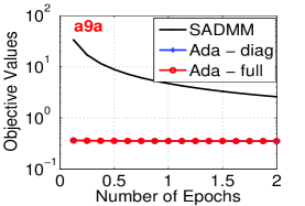
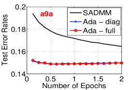
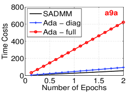
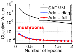
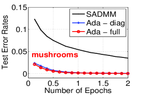
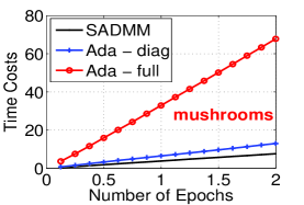
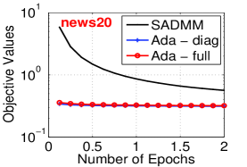
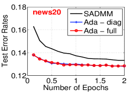
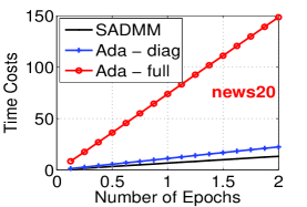
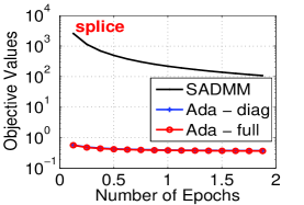
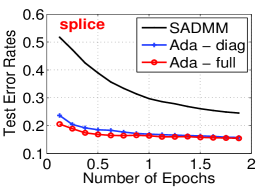
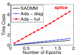
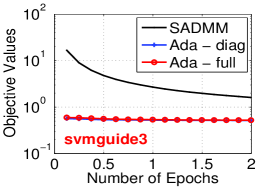
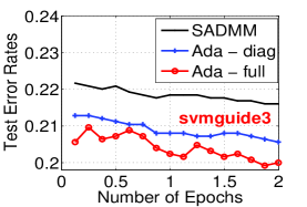
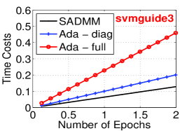
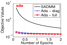
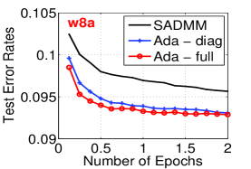
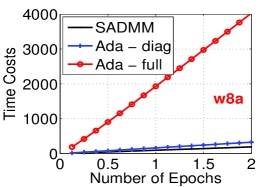
Figure 1: Comparison between SADMM with Ada-SADMM_diag (“Ada-diag”) and Ada-SADMM_full (“Ada-full”) on 6 real-world datasets. Epoch for the horizontal axis is the number of iterations divided by dataset size. Left Panels: Average objective values. Middle Panels: Average test error rates. Right Panels: Average time costs (in seconds).

4 Conclusion

ADMM is a popular technique in machine learning. This paper studied to accelerate stochastic ADMM with adaptive subgradient, by replacing the fixed proximal function with adaptive proximal function. Compared with traditional stochastic ADMM, we show that the proposed adaptive algorithms converge significantly faster through the proposed adaptive strategies. Promising experimental results on a variety of real-world datasets further validate the effectiveness of our techniques.

References

- [1] Stephen Boyd, Neal Parikh, Eric Chu, Borja Peleato, and Jonathan Eckstein. Distributed optimization and statistical learning via the alternating direction method of multipliers. Foundations and Trends® in Machine Learning, 3(1):1–122, 2011.
- [2] Wei Deng and Wotao Yin. On the global and linear convergence of the generalized alternating direction method of multipliers. Technical report, DTIC Document, 2012.
- [3] John Duchi, Elad Hazan, and Yoram Singer. Adaptive subgradient methods for online learning and stochastic optimization. The Journal of Machine Learning Research, 999999:2121–2159, 2011.
- [4] Jonathan Eckstein and Dimitri P Bertsekas. On the douglas rachford splitting method and the proximal point algorithm for maximal monotone operators. Mathematical Programming, 55(1-3):293–318, 1992.
- [5] Jerome Friedman, Trevor Hastie, and Robert Tibshirani. Sparse inverse covariance estimation with the graphical lasso. Biostatistics, 9(3):432–441, 2008.
- [6] Daniel Gabay. Chapter ix applications of the method of multipliers to variational inequalities. Studies in mathematics and its applications, 15:299–331, 1983.
- [7] Daniel Gabay and Bertrand Mercier. A dual algorithm for the solution of nonlinear variational problems via finite element approximation. Computers & Mathematics with Applications, 2(1):17–40, 1976.
- [8] R. Glowinski and A. Marroco. Sur lapproximation, par elements nis dordre un, et la resolution, par penalisationdualite, dune classe de problems de dirichlet non lineares. Revue Francaise dAutomatique, Informatique, et, 1975.
- [9] Roland Glowinski and Patrick Le Tallec. Augmented Lagrangian and operator-splitting methods in nonlinear mechanics, volume 9. SIAM, 1989.
- [10] Donald Goldfarb, Shiqian Ma, and Katya Scheinberg. Fast alternating linearization methods for minimizing the sum of two convex functions. Math. Program., 141(1-2):349–382, 2013.
- [11] Tom Goldstein and Stanley Osher. The split bregman method for l1-regularized problems. SIAM Journal on Imaging Sciences, 2(2):323–343, 2009.
- [12] Bingsheng He and Xiaoming Yuan. On the o(1/n) convergence rate of the douglas-rachford alternating direction method. SIAM Journal on Numerical Analysis, 50(2):700–709, 2012.
- [13] Zhi-Quan Luo. On the linear convergence of the alternating direction method of multipliers. arXiv preprint arXiv:1208.3922, 2012.
- [14] Renato D. C. Monteiro and Benar Fux Svaiter. Iteration-complexity of block-decomposition algorithms and the alternating direction method of multipliers. SIAM Journal on Optimization, 23(1):475–507, 2013.
- [15] Hua Ouyang, Niao He, Long Tran, and Alexander G Gray. Stochastic alternating direction method of multipliers. In Proceedings of the 30th International Conference on Machine Learning (ICML-13), pages 80–88, 2013.
- [16] Taiji Suzuki. Dual averaging and proximal gradient descent for online alternating direction multiplier method. In Proceedings of the 30th International Conference on Machine Learning (ICML-13), pages 392–400, 2013.
- [17] Huahua Wang and Arindam Banerjee. Online alternating direction method. In Proceedings of the 29th International Conference on Machine Learning (ICML-12), pages 1119–1126, 2012.
- [18] Junfeng Yang and Yin Zhang. Alternating direction algorithms for -problems in compressive sensing. SIAM journal on scientific computing, 33(1):250–278, 2011.