Closed-loop liquid-liquid immiscibility in mixture of particles with spherically symmetric interaction

Abstract

Thermodynamic perturbation theory for central-force (TPT-CF) type of associating potential is used to study the phase behavior of symmetric binary mixture of associating particles with spherically symmetric interaction. The model is represented by the binary Yukawa hard-sphere mixture with additional spherically symmetric square-well associative interaction located inside the hard-core region and valid only between dissimilar species. To account for the change of the system packing fraction due to association we propose an extended version of the TPT-CF approach. In addition to the already known four types of the phase diagram for binary mixtures we were able to identify the fifth type, which is characterized by the absence of intersection of the $\lambda$-line with the liquid-vapour binodals and by the appearance of the closed- loop liquid-liquid immiscibility with upper and lower critical solution temperatures.

Key words: thermodynamic perturbation theory, liquid-vapour coexistence, demixing, binary mixture, associating fluids

PACS: 64.70.Ja, 05.70.Jk, 82.70.Dd, 64.10.+h

Abstract

В рамках термодинамiчної теорiї збурень для асоцiативного потенцiалу типу центральних сил проведено дослiдження фазової поведiнки симетричної бiнарної сумiшi асоцiативних частинок з сферично-симетричною взаємодiєю. Модель представлено бiнарною сумiшшю юкавiвських твердих сфер з додатковою сферично-симетричною асоцiативною взаємодiєю типу прямокутної ями, яка розмiщена усерединi областi твердої сфери i дiє тiльки мiж рiзними сортами. Враховуючи змiну упаковки системи внаслiдок асоцiацiї, запропоновано узагальнення термодинамiчної теорiї збурень для асоцiативного потенцiалу типу центральних сил. На додаток до чотирьох вже вiдомих типiв фазових дiаграм для бiнарних сумiшей, нам вдалося визначити п’ятий тип, який характеризується вiдсутнiстю перетину лямбда-лiнiї з бiнодалями ‘‘рiдина-газ’’ i появою незмiшування ‘‘рiдина-рiдина’’ у виглядi замкненої петлi з верхньою i нижньою критичними температурами змiшування.

Ключовi слова: термодинамiчна теорiя збурень, спiвiснування ‘‘рiдина-газ’’, розшаровування, бiнарна сумiш, асоцiативнi рiдини

1 Introduction

According to the Gibbs phase rule, the binary mixture may have up to four coexisting phases simultaneously. This fact implies that the phase behavior of the binary fluid could be very rich and complicated. Systematic study and classification of the peculiarities of the binary systems phase diagrams topologies has been undertaken more than 40 years ago by Scott and van Konynenburg [1, 2]. These studies are based on the application of the van der Waals equation of state, which in most cases is capable of providing qualitatively correct description of the phase behavior. Most of the subsequent studies, carried out using quantitatively more accurate methods of the modern liquid state theory [3], have been focused on the investigation of the phase behavior of symmetric binary mixtures [4, 5, 6, 7]. These are the mixtures with identical interaction between particles of the similar species and different interaction between particles of the dissimilar species. Phase behavior of such mixtures is defined by the competition between gas-liquid and liquid-liquid coexistence. Combining Monte-Carlo computer simulation and theoretical mean-field calculations, Wilding et al. [4] identified three types of a phase diagram for square-well hard-sphere symmetrical binary fluid mixture. Similar three types of a phase diagram were detected in the symmetrical binary hard-sphere Yukawa mixture using self-consistent Ornstein-Zernike approximation (SCOZA) and Monte-Carlo computer simulation method [5, 6]. At the same time, the phase diagram of the fourth type was also detected using SCOZA approach [8]. More recently, the first-order thermodynamic perturbation theory has been used to study the phase behavior of the binary Yukawa mixture with asymmetry in hard-sphere sizes [7].

In this study we are focused on the investigation of the phase behavior of symmetric Yukawa hard-sphere binary mixture with additional spherically symmetric square-well associative interaction located inside the hard-core region. This additional interaction is valid only between particles of dissimilar species. The hard-sphere version of the model has been developed and studied by Cummings and Stell [9] and by Kalyuzhnyi et al. [10]. Originally, this version of the model was used as a simple hamiltonian model of the chemical reaction [9]. On the other hand, the model of this type can be regarded as a coarse grained version of the model for sterically or charge stabilized colloidal dispersions, protein solutions, star-polymer fluids, etc. [11, 12, 13]. Effective interaction between macroparticles of such systems has an attractive potential well at short distances and a repulsive potential mound at intermediate distances. The phase diagrams, which include two-phase gas-liquid, liquid-liquid diagrams and three-phase gas-demixed liquid diagrams have been calculated using thermodynamic perturbation theory for central force associating potential [14, 15, 16].

Phase behavior of the model, which is similar to the present one has been studied earlier by Jakson [17]. His model is represented by the symmetrical binary hard-sphere mixture with mean-field type of attractive interaction valid only between the same species and orientationally dependent associative interaction between particles of unlike species. Associative interaction appears due to the off-center square-well sites. This model was used as a generic model for the phase behavior description of the binary mixtures with the possibility of hydrogen bond formation between unlike species. Combining Wertheim’s TPT for associating fluids and mean-field approach, Jackson was able to show that for a certain choice of the potential model parameters, the system exhibits the closed loop liquid-liquid immiscibility with the upper and lower critical solution temperatures. It was concluded that closed loop coexistence appeares due to the presence of the highly anysotropic attraction between off-center bonding sites.

In the present work we demonstrate that the systems with spherically symmetric interaction may also have closed loop liquid-liquid immiscibility. The paper is organized as follows. In section 2 we describe the model to be considered and in section 3 we present and discuss details of the TPT-CF theory, specialized to the model at hand. Our results and discussion are included in section 4 and our conclusions are collected in section 5.

2 The model

We consider symmetric binary Yukawa hard-sphere mixture with additional associative interaction between dissimilar particles. The total pair potential of the model $U_{ij}(r)$ is represented as a sum of hard-sphere Yukawa potential $U_{ij}^{\textrm{HSY}}(r)$ and associative potential $U_{\textrm{ass}}(r)$, i.e.:

$$U_{ij}(r)=U_{ij}^{\textrm{HSY}}(r)+(1-\delta_{ij})U_{\textrm{ass}}(r),$$ (2.1)

where the lower indices $i,j$ denote the species of the particles and $\delta_{ij}$ is the Kroneker delta. In our symmetric binary system, Yukawa interaction between particles of the same species is the same, i.e., $U_{11}^{\textrm{HSY}}(r)=U_{22}^{\textrm{HSY}}(r)$, and between the particles of dissimilar species it is regulated by the parameter $\alpha$ ($0<\alpha<1$), i.e. $U_{12}^{\textrm{HSY}}(r)=\alpha U_{11}^{\textrm{HSY}}(r)$. We have:

$$U_{ii}^{\textrm{HSY}}(r)=\left\{\begin{array}[]{ll}\infty,&\hbox{$r\leqslant d_{ii}$}\,,\\ -\frac{\epsilon_{0}}{r}\frac{A_{ii}}{z_{n}}\mathrm{e}^{-z_{n}(r-d_{ii})},&\hbox{$r>d_{ii}$}\,,\end{array}\right.$$ (2.2)

$$U_{12}^{\textrm{HSY}}(r)=U_{21}^{\textrm{HSY}}(r)=\left\{\begin{array}[]{ll}\infty,&\hbox{$r<L-\omega/2$}\,,\\ A_{0},&\hbox{$L-\omega/2<r<d_{12}$}\,,\\ -\frac{\epsilon_{0}}{r}\frac{A_{12}}{z_{n}}\mathrm{e}^{-z_{n}(r-d_{12})},&\hbox{$r>d_{12}$}\,,\end{array}\right.$$ (2.3)

where $A_{11}=A_{22}=dz_{n}$, $A_{12}=A_{21}=\alpha A_{11}$, $z_{n}$ and $\epsilon_{0}$ are the screening length and the interaction strength of the Yukawa potential, respectively, $d_{ij}=(d_{i}+d_{j})/2$, $d_{i}$ is the hard-sphere diameter. We consider the system with hard spheres of equal size, i.e., $d_{1}=d_{2}=d$. In (2.1)

$$U_{\textrm{ass}}(r)=\left\{\begin{array}[]{ll}0\,,&\hbox{$r<L-\omega/2$}\,,\\ -\varepsilon_{\textrm{ass}}-A_{0}\,,&\hbox{$L-\omega/2<r<L+\omega/2$}\,,\\ 0\,,&\hbox{$r>L+\omega/2$}\,,\end{array}\right.$$ (2.4)

where $L$ is the bonding distance, $\omega$ and $\varepsilon_{\textrm{ass}}$ are the square well potential width and depth, respectively. In what follows we will consider the hard-sphere Yukawa potential (2.2) and (2.3) in the limit of $A_{0}\rightarrow\infty$, and associative potential (2.4) in the limit of sticky interaction under the condition that the second virial coefficient remains unchanged. In this limit, the Mayer function for associative potential $f_{\textrm{ass}}(r)=\exp{[-\beta U_{\textrm{ass}}(r)]}-1$ is substituted by the Dirac delta-function, i.e., $e_{12}^{(\textrm{HSY})}(r)f_{\textrm{ass}}(r)\rightarrow B\delta(r-L)$, where $e_{12}^{(\textrm{HSY})}(r)=\exp{[-\beta U_{12}^{(\textrm{HSY})}(r)]}$ and

$$B=L^{-2}\int r^{2}e_{12}^{(\textrm{HSY})}(r)f_{\textrm{ass}}(r)\;\mathrm{d}r.$$ (2.5)

The type of the clusters, which will be formed in the system due to association depends on the value of the bonding length $L$ [14, 10]. For values of L lying in the interval $(0,d/2)$ only dimers can be formed in the system. When $d/2<L<\sqrt{3}d$, the formation of the chains is possible. Further increase in $L$ leads to an increase in the maximum number of the particles of the type 1 (or 2), which can be simultaneously associated with the particle of the type 2 (or 1), and the formation of the branched chains will be possible.

The mixture is characterized by the temperature $T$ (or $\beta=(k_{\textrm{B}}T)^{-1}$, where $k_{\textrm{B}}$ is the Boltzmann’s constant), the total number-density $\rho$, and the mole (number) fraction $x$ of species $1$ ($x=x_{1}$); partial number densities are defined via $\rho_{1}=x\rho$ and $\rho_{2}=(1-x)\rho$. We further introduce the reduced dimensionless quantities, $\rho^{*}=\rho d^{3}$, $T^{*}=k_{\textrm{B}}T/\epsilon_{0}$ and $\epsilon_{\textrm{ass}}^{*}=\epsilon_{\textrm{ass}}/\epsilon_{0}$.

3 Theory

To describe thermodynamic properties of the model at hand we will utilize here thermodynamic perturbation theory for central force associative potential (TPT-CF) [14, 15, 16]. According to TPT-CF, Helmholtz free energy of the system $A$ can be written as a sum of two terms: free energy of the reference system $A_{\textrm{ref}}$ and the term describing the contribution to the free energy due to association $A_{\textrm{ass}}$:

$$A=A_{\textrm{ref}}+A_{\textrm{ass}}=A_{\textrm{HSY}}+A_{\textrm{ass}}\,.$$ (3.1)

Here, $A_{\textrm{ref}}=A_{\textrm{HSY}}$, where $A_{\textrm{HSY}}$ is the free energy of the hard-sphere Yukawa fluid. To calculate $A_{\textrm{HSY}}$, we are using the high temperature approximation. All the rest of thermodynamical quantities can be obtained using the expression for Helmholtz free energy (3.1) and standard thermodynamical relations, e.g., differentiating $A$ with respect to the density, we get the expression for the chemical potential:

$$\beta\mu_{k}=\frac{\partial}{\partial\rho_{k}}\bigg{(}\frac{\beta A}{V}\bigg{)},$$ (3.2)

and the expression for the pressure $P$ of the system can be calculated invoking the following general relation:

$$\beta P=\beta\sum_{k}\rho_{k}\mu_{k}-\frac{\beta A}{V}\,.$$ (3.3)

3.1 High temperature approximation

Under the high temperature approximation, the expression for the free energy is:

$$\frac{\beta A_{\textrm{HSY}}}{V}=\frac{\beta A_{\textrm{HS}}}{V}+2\pi\beta\sum_{i}\sum_{j}\rho_{i}\rho_{j}\int_{0}^{\infty}\mathrm{d}rr^{2}U_{ij}^{\textrm{HSY}}(r)g_{\textrm{HS}}(r),$$ (3.4)

where $A_{\textrm{HS}}$ is the hard-sphere Helmholtz free energy and $g_{\textrm{HS}}(r)$ is the hard-sphere radial distribution function. Substituting into (3.4) the expression for the potential (2.2) and (2.3), we have

$$\frac{\beta A_{\textrm{HSY}}}{V}=\frac{\beta A_{\textrm{HS}}}{V}-{2\pi\beta\epsilon_{0}\over z_{n}}\widetilde{G}_{\textrm{HS}}(z_{n})\sum_{i}\sum_{j}\rho_{i}\rho_{j}A_{ij}\,,$$ (3.5)

where $\widetilde{G}_{\textrm{HS}}(z_{n})$ is the Laplace transform of hard-sphere radial distribution function

$$\widetilde{G}_{\textrm{HS}}(z_{n})=\mathrm{e}^{z_{n}d_{ij}}\int_{0}^{\infty}\mathrm{d}rr\mathrm{e}^{-z_{n}r}g_{\textrm{HS}}(r).$$ (3.6)

Here, we will be using Percus-Yevick expression for $\widetilde{G}_{\textrm{HS}}(z_{n})$, i.e.,

$$\widetilde{G}_{(\textrm{HS})}(z_{n})=\frac{[\lambda_{2}+z_{n}(\lambda_{1}+\lambda_{2})]}{z_{n}^{2}\widetilde{D}_{0}^{(n)}}\,,$$ (3.7)

where

$$\lambda_{1}=-\frac{3}{2}\frac{\eta}{(1-\eta)^{2}}\,,\qquad\lambda_{2}=\frac{1+2\eta}{(1-\eta)^{2}}\,,$$ (3.8)

$$\widetilde{D}_{0}^{(n)}=\left\{1-12\eta\left[\frac{\lambda_{1}+\lambda_{2}}{z_{n}^{2}}\left(1-z_{n}d-\mathrm{e}^{-z_{n}d}\right)+\frac{\lambda_{2}}{z_{n}^{3}}\bigg{(}1-z_{n}d+\frac{z_{n}^{2}}{2}-\mathrm{e}^{-z_{n}d}\bigg{)}\right]\right\}$$ (3.9)

and $\eta=\pi(\rho_{1}+\rho_{2})d^{3}/6$.

Differentiating the expression for Helmholtz free energy (3.4) with respect to the density, we get the following expression for the chemical potential:

$$\beta\mu_{k}^{(\textrm{HSY})}=\frac{\partial}{\partial\rho_{k}}\bigg{(}\frac{\beta A_{\textrm{HSY}}}{V}\bigg{)}=\beta\mu_{k}^{(\textrm{HS})}+\beta\Delta\mu_{k}^{(\textrm{HSY})},$$ (3.10)

where $\mu_{k}^{\textrm{HSY}}$ is the hard-sphere chemical potential and

$$\beta\Delta\mu_{k}^{(\textrm{HSY})}=-\frac{2\pi\beta\epsilon_{0}}{z_{n}}\left[{\partial\widetilde{G}_{\textrm{HS}}(z_{n})\over\partial\rho_{k}}\sum_{i}\sum_{j}\rho_{i}\rho_{j}A_{ij}+2\widetilde{G}_{\textrm{HS}}(z_{n})\sum_{i}\rho_{i}A_{ik}\right].$$ (3.11)

Pressure $P_{\textrm{HSY}}$ of the system can be calculated invoking the following general relation:

$$\beta P_{\textrm{HSY}}=\beta\sum_{k}\rho_{k}\mu_{k}^{(\textrm{HSY})}-\frac{\beta A_{\textrm{HSY}}}{V}\,.$$ (3.12)

In the above expressions, $A_{\textrm{HS}}$ and $\mu_{k}^{(\textrm{HS})}$ are calculated using the corresponding Carnahan-Starling expressions [18].

3.2 Thermodynamic perturbation theory

According to the TPT-CF for the associative part of the free energy $A_{\textrm{ass}}$, we have:

$$\frac{\beta A_{\textrm{ass}}}{V}=\sum_{k}\left[\rho_{k}\ln\left(\frac{\sigma^{(0)}_{k}}{\rho_{k}}\right)+\frac{1}{2}\sigma^{(m-1)}_{k}\frac{\sigma^{(1)}_{k}-\sigma^{(0)}_{k}}{\sigma^{(0)}_{k}}\right],$$ (3.13)

where

$$\sigma^{(l)}_{k}=\sigma^{(0)}_{k}\sum_{n=0}^{l}\frac{1}{n!}\left(\frac{\sigma^{(1)}_{k}-\sigma^{(0)}_{k}}{\sigma^{(0)}_{k}}\right)^{n}\qquad\text{for}\qquad l=2,\ldots,m\,.$$ (3.14)

Here, $m$ is the maximum number of associative bonds per particle (the maximum number of the particles, which can be bonded to a given particle simultaneously), $\sigma^{(l)}_{k}=\sum_{l}\rho^{(l)}_{k}$, $\rho_{k}=\sum_{l}\rho_{k}^{(l)}$ and $\rho^{(l)}_{k}$ is the density of $l$-times bonded particles. For the present two-component mixture, the density parameters $\sigma_{k}^{(0)}$ and $\sigma_{k}^{(1)}$ satisfy the following set of equations

$$\left\{\begin{array}[]{ll}\frac{\sigma_{1}^{(1)}-\sigma_{1}^{(0)}}{\sigma_{1}^{(0)}}=\left[\rho_{2}-\frac{1}{m!}\frac{\left(\sigma_{2}^{(1)}-\sigma_{2}^{(0)}\right)^{m}}{\left(\sigma_{2}^{(0)}\right)^{m-1}}\right]K,\\[8.61108pt] \rho_{1}\left(\sigma_{1}^{(0)}\right)^{m-1}=\sum_{k=0}^{m}\frac{(\sigma_{1}^{(0)})^{k}}{(m-k)!}\left(\sigma_{1}^{(1)}-\sigma_{1}^{(0)}\right)^{m-k},\\[8.61108pt] \frac{\sigma_{2}^{(1)}-\sigma_{2}^{(0)}}{\sigma_{2}^{(0)}}=\left[\rho_{1}-\frac{1}{m!}\frac{\left(\sigma_{1}^{(1)}-\sigma_{1}^{(0)}\right)^{m}}{\left(\sigma_{1}^{(0)}\right)^{m-1}}\right]K,\\[8.61108pt] \rho_{2}\left(\sigma_{2}^{(0)}\right)^{m-1}=\sum_{k=0}^{m}\frac{\left(\sigma_{2}^{(0)}\right)^{k}}{(m-k)!}\left(\sigma_{2}^{(1)}-\sigma_{2}^{(0)}\right)^{m-k},\end{array}\right.$$ (3.15)

where

$$K=4\pi\int y^{(00)}_{12}(r)e^{(\textrm{HSY})}(r)f_{\textrm{ass}}(r)r^{2}\mathrm{d}r=4\pi BL^{2}y^{(00)}_{12}(L),$$ (3.16)

$y^{(00)}_{12}(r)$ represent the cavity distribution function between two Yukawa hard spheres of species 1 and 2 infinitely diluted in the original associating fluid in question. Usually, this function is approximated by the hard-sphere Yukawa cavity correlation function $y_{12}^{(\textrm{HSY})}(r,\eta)$ calculated for the packing fraction $\eta$. This appears to be a good approximation for the models with bonding length $L\approx d$, since in this case $y^{(00)}_{12}(r)$ only weakly depends on the degree of the system association. However, for $L<d$, the actual (effective) packing fraction $\eta_{\textrm{eff}}$ and thus $y^{(00)}_{12}(r)$ are strongly dependent on the system degree of association, and the usual approximation becomes inadequate. In the present study we propose to approximate $y^{(00)}_{12}(r)$ by the hard-sphere Yukawa cavity correlation function $y_{12}^{(\textrm{HSY})}(r,\eta_{\textrm{eff}})$ calculated for the effective packing fraction $\eta_{\textrm{eff}}$, i.e.,

$$\eta_{\textrm{eff}}=\frac{\pi d^{3}}{6}\sum_{k}\rho_{k}X_{k}^{(0)}+\sum_{n=1}^{m}\left(\frac{\pi d^{3}}{6}-nV_{\textrm{exc}}\right)\sum_{k}\frac{\rho_{k}X^{(0)}_{k}}{n!}\left(\frac{X^{(1)}_{k}}{X^{(0)}_{k}}\right)^{n},$$ (3.17)

where the excluded volume $V_{\textrm{exc}}$ is:

$$V_{\textrm{exc}}=\frac{\pi}{24}(d-L)^{2}(2d+L).$$ (3.18)

$X_{k}^{(0)}=\rho_{k}^{(0)}/\rho_{k}$ and $X_{k}^{(1)}=\rho_{k}^{(1)}/\rho_{k}$. According to this expression, $\eta_{\textrm{eff}}$ [and thus $y_{12}^{(\textrm{HSY})}(r)$] depends on the degree of association of the system represented by the fractions of free $X_{k}^{(0)}$ and singly bonded $X_{k}^{(1)}$ particles.

In the present study, the solution of this equation is obtained via numerical iteration method. On each iteration step, the new estimate for the fractions $X^{(l)}_{k,\textrm{new}}$ $(l=0,1)$ is calculated by solving the following set of equations:

$$\left\{\begin{array}[]{ll}\frac{X_{1,\textrm{new}}^{(1)}}{X_{1,\textrm{new}}^{(0)}}=\left[1-\frac{1}{m!}\frac{\left(X_{2,\textrm{new}}^{(1)}\right)^{m}}{\left(X_{2,\textrm{new}}^{(0)}\right)^{m-1}}\right]\rho_{2}K\left[\eta_{\textrm{eff}}(X_{\textrm{old}})\right],\\[12.91663pt] \left(X_{1,\textrm{new}}^{(0)}\right)^{m-1}=\sum_{n=0}^{m}\frac{\left(X_{1,\textrm{new}}^{(0)}\right)^{n}}{(m-n)!}\left(X_{1,\textrm{new}}^{(1)}\right)^{m-n},\\[8.61108pt] \frac{X_{2,\textrm{new}}^{(1)}}{X_{2,\textrm{new}}^{(0)}}=\left[1-\frac{1}{m!}\frac{\left(X_{1,\textrm{new}}^{(1)}\right)^{m}}{\left(X_{1,\textrm{new}}^{(0)}\right)^{m-1}}\right]\rho_{1}K\left[\eta_{\textrm{eff}}(X_{\textrm{old}})\right],\\[12.91663pt] \left(X_{2,\textrm{new}}^{(0)}\right)^{m-1}=\sum_{n=0}^{m}\frac{\left(X_{2,\textrm{new}}^{(0)}\right)^{n}}{(m-n)!}\left(X_{2,\textrm{new}}^{(1)}\right)^{m-n},\end{array}\right.$$ (3.19)

which is obtained using a set of equations (3.15). Here, $X_{\textrm{old}}$ is the value of $X$ calculated during the previous iteration step. Our iteration loop consists of two steps. In the first step, the current value of $\eta_{\textrm{eff}}$ is used to calculate the new values of $X_{k}^{(l)}$ using the set of equation (3.19). On the second step, we insert these values of $X_{k}^{(l)}$ into the right-hand side of the relation (3.17) to get a new estimate for $\eta_{\textrm{eff}}$. This iteration loop is repeated until the following condition

$${\frac{|\eta_{\textrm{eff},\textrm{new}}-\eta_{\textrm{eff,old}}|}{\eta_{\textrm{eff},\textrm{new}}+\eta_{\textrm{eff,old}}}}\leqslant 10^{-8}$$ (3.20)

is satisfied. For the initial guess we have used the value of $\eta_{\textrm{eff}}=\eta$.

3.3 The cavity correlation function for Yukawa hard sphere fluid

The cavity correlation function $y_{12}^{(\textrm{HSY})}(r)$, which is needed to solve the set of equations for the fractions $X_{k}^{(l)}$ (3.19) is calculated using the reference hypernetted chain type of approximation

$$y_{ij}^{(\textrm{HSY})}(r)=y_{ij}^{(\textrm{HS})}(r)\exp{\left[\delta h_{ij}^{(\textrm{HSY})}(r)-\delta c_{ij}^{(\textrm{HSY})}(r)\right]},\;\;\;\;\;\;$$ (3.21)

where $y_{ij}^{(\textrm{HS})}(r)$ is the hard-sphere cavity correlation function, $\delta h_{ij}^{(\textrm{HSY})}(r)=h_{ij}^{(\textrm{HSY})}(r)-h_{ij}^{(\textrm{HS})}(r)$ and $\delta c_{ij}^{(\textrm{HSY})}(r)=c_{ij}^{(\textrm{HSY})}(r)-c_{ij}^{(\textrm{HS})}(r)$. Here, the upper indices (HS) and (HSY) denote the hard-sphere and hard-sphere Yukawa quantities, respectively, and $h$ and $c$ denote total and direct correlation functions, respectively. In the hard-core region $\delta h_{ij}^{(\textrm{HSY})}(r)=0$ and for $\delta c_{ij}^{(\textrm{HSY})}(r)$, we have used the expression obtained in the framework of the first-order mean spherical approximation [19]. The hard-sphere cavity correlation function $y_{ij}^{(\textrm{HS})}(r)$ was calculated using Henderson-Grundke approximation [20]. Closed form analytical expressions for $\delta c_{ij}^{(\textrm{HSY})}(r)$ and $y_{ij}^{(\textrm{HS})}(r)$ are presented in the appendix.

3.4 Calculation of the phase diagram

Our calculation of the phase diagram follows closely the scheme, proposed in [5]. It is based on the solution of the set of equations that follow from the conditions of phase equilibrium, i.e., equal chemical potentials and pressures of the coexisting phases at a given temperature. The coexisting phases are characterized by $(\rho,x)$ and $(\rho^{\prime},x^{\prime})$. From the Gibbs’ phase rule, we expect up to four phases to be in equilibrium, i.e., the vapour (V), the mixed fluid (MF), and two (symmetric) phases of the demixed fluid (DF).

The V-MF transition is obtained by solving the set of equations:

$$\mu_{i}(\rho,T,x=1/2)\equiv\mu(\rho,T,x=1/2)=\mu(\rho^{\prime},T,x=1/2),$$ (3.22)

$$P(\rho,T,x=1/2)=P(\rho^{\prime},T,x=1/2).$$ (3.23)

The V-MF and MF-DF transitions are obtained in two steps: first we determine the phase diagram of the demixing transitions , i.e., looking at a given temperature $T$ for two coexisting states with the same fluid density but different composition by fixing $\rho=\rho^{\prime}$ and by determining concentrations $x$ and $x^{\prime}=1-x$ of the coexisting phases. The equilibrium condition for the pressure is automatically fulfilled, while the equilibrium condition for the chemical potentials takes place at given $T$ and $\rho$

$$\mu(\rho,T,x)=\mu(\rho,T,x),$$ (3.24)

which defines the line $x(\rho)$ of the second order transition.

In the second step, the solution of the two equations

$$\mu[\rho,T,x=1/2] =\mu[\rho^{\prime},T,x(\rho^{\prime})],$$ (3.25)

$$P[\rho,T,x=1/2] =P[\rho^{\prime},T,x(\rho^{\prime})]$$ (3.26)

gives the density $\rho$ of the V or MF and the density of the DF with concentrations $x(\rho^{\prime})$ and $1-x(\rho^{\prime})$, in equilibrium.

4 Results and discussion

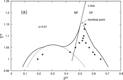
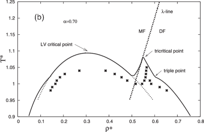
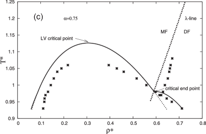
Figure 1: Phase diagram of the symmetric binary Yukawa hard-sphere associating mixture in $\rho^{*}$ vs $T^{*}$ coordinate frame for $\epsilon^{*}=0$ and $\alpha=0.65$ (panel a), $\alpha=0.7$ (panel b) and $\alpha=0.75$ (panel c). Lines represent the results of the present theory and symbols depict MC computer simulation results [8]. Here, dashed lines denote the $\lambda$-lines and dotted lines show the metastable LV binodals.

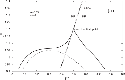
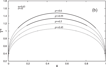
Figure 2: Phase diagram of the symmetric binary Yukawa hard-sphere associating mixture in $\rho^{*}$ vs $T^{*}$ coordinate frame (panel a) and in $x$ vs $T^{*}$ frame for different values of the density $\rho^{*}$ (panel b) at $\epsilon^{*}=0$ and $\alpha=0.63$. Dashed lines denote the $\lambda$-line and solid and dotted lines represent stable and unstable portions of the coexisting densities (panel a) and coexisting mole (number) fractions (panel b), respectively.

In this section we present our numerical results for the phase behavior of the model in question. All the calculations are carried out at Yukawa screening parameter $z_{n}d=1.8$ and square-well width $\omega=0.0000404981$.

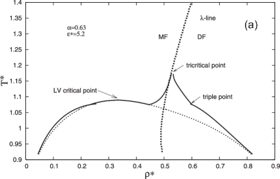
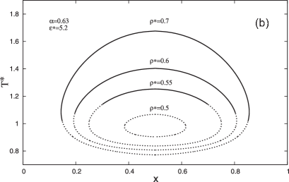
Figure 3: The same as in figure 2 at $\epsilon^{*}=5.2$ and $\alpha=0.63$.

According to the previous studies [10], predictions of our theory for thermodynamical properties of the model with $A_{ij}=0$ are in a good agreement with computer simulation predictions. To test the accuracy of the theory for the model with $\epsilon_{\textrm{ass}}^{*}=0$, we compare theoretical and computer simulation predictions for its phase behavior. In figure 1 we show the phase diagram of the system at $\epsilon_{\textrm{ass}}^{*}=0$ and three values of $\alpha$, i.e., $\alpha=0.65,\;0.7,\;0.75$. These are the system parameters for which the three types of the phase diagram were identified [4, 5], depending on the position of intersection point of the $\lambda$-line, which represent the second-order demixing transition, with the binodals of the liquid-vapour (LV) phase transition. In addition, for comparison in the same figure, we present the corresponding computer simulations results [6]. Overall there is a reasonably good qualitative agreement between theoretical and computer simulation predictions. Predictions of the theory in the region of the LV critical point are about $6\%$ higher than those of the computer simulation. As a result, while the types I and II of the phase diagrams (according to the nomenclature of references [4, 5]) are theoretically reproduced for the set of the potential model parameters used to simulate the type III of the diagram, theoretical calculations still show the type II of the diagram with a small portion of stable binodals in the vicinity of the LV critical point. However, it is quite obvious that a small decrease in $\alpha$ will cause the theoretical phase diagram to change its type from type II to type III. This can be seen in figure 2 (panel a), where our results for $\alpha=0.63$ are shown. In the phase diagram of the type I the LV, coexistence is unstable with respect to the three-phase coexistence between mixed fluid (MF) and demixed fluid (DF) and the $\lambda$-line ends at the tricritical point. In the type II of the diagram, $\lambda$-line ends also at the tricritical point, however, there is a portion of the LV phase diagram beeing stable in the range of the temperatures between the critical temperature and the temperature of the triple point, where one can observe LV coexistence at lower densities. Between tricritical temperature and temperature of the triple point, the MF-DF three-phase coexistence can be seen. At the triple point, there is a four-phase vapour, MF and DF coexistence. In the case of the type II diagram, the $\lambda$-line intersects the liquid binodal at the temperature slightly below the critical. In the type III of the diagram, the $\lambda$-line intersects the liquid binodal at the temperature well below the critical temperature. Here, we can see the critical end point below which there is a three phase V-DF coexistence and above which (up to the LV critical temperature), there is a LV coexistence. In the type IV of the diagram, the $\lambda$-line intersects LV binodals at the densities that are lower than the LV critical densities [8]. This occures at $\alpha=0$. We have also detected this type of the diagram, using the current approach; however, the results are not shown here.

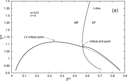
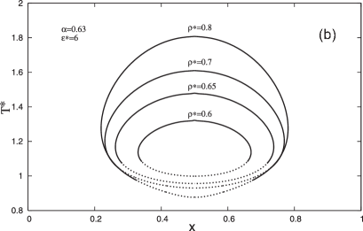
Figure 4: The same as in figure 2 at $\epsilon^{*}=6$ and $\alpha=0.63$.

Next, we proceed to the discussion of the phase diagrams for the nonzero value of the strength of associating interaction $\epsilon^{*}=5.2,\;6.0,\;6.5$ at $\alpha=0.63$ (figures 3–5). Unfortunately, computer simulation results for the phase behavior of the model at hand are not available. However, taking into account a reasonable performance of the theory in the two limiting cases discussed above ($A_{ij}=0$ and $\epsilon_{0}=0$), we expect that the accuracy of the theory for the full version of the model will be satisfactory as well. In figures 3–5, we depict the phase diagram in $\rho^{*}$ vs $T^{*}$ (panel a) and $x$ vs $T^{*}$ at different values of the density (panel b) frames. For $\epsilon=0$ and $\alpha=0.63$, temperature-concentration slices of the phase diagram at different densities are also shown (panel b in figure 2). In the latter case, only the upper portions of the corresponding coexistence curves for $\rho^{*}=0.55,\;0.6$ are stable. The lower portions of these curves and the demixing curves for $\rho^{*}=0.5,\;0.45$ are unstable with respect to the three-phase MF-DF coexistance. With the temperature decrease, the difference in the compositions of the coexisting liquids increases. With the increase of the strength of association $\epsilon^{*}$, the topology of the phase behavior in $T^{*}$ vs $\rho^{*}$ coordinate frame changes from the type III (figure 2) to type II at $\epsilon^{*}=5.2$ (figure 3) and next to type I at $\epsilon^{*}=6.0$ (figure 4). At the same time, one can observe the appearance of the closed loop liquid-liquid immiscibility curves with the upper stable and lower unstable critical solution points (figures 3 and 4). The stable portion of the curves increases with an increasing strength of associative interaction. Finally, for $\epsilon^{*}=6.5$, the closed-loop coexistence curves for demixing coexistence becomes stable (figure 5, panel b). This corresponds to the situation when there is no intersection between LV binodals a $\lambda$-line (figure 5, panel a). Thus, for these values of the potential model parameters, in addition to already identified four types of the phase diagram, we have identified one more, which we call the type V of the two-component mixture phase diagram topology. In a future we are planning to extend and apply our approach to study the effects of the external field [21] and porous media [22, 23] on the phase behaviour of the current model.

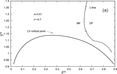
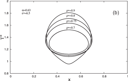
Figure 5: The same as in figure 2 at $\epsilon^{*}=6.5$ and $\alpha=0.63$.

5 Conclusions

In this paper we have used the TPT-CF approach to study the phase behavior of a symmetric two-component Yukawa mixture of associating particles with spherically symmetric interaction. Our theoretical predictions for the phase diagram of the version of the model without association appear to be in reasonably good qualitative agreement with the predictions of the corresponding Monte-Carlo computer simulation method [6]. For the model with nonzero associating potential, we were able to identify, in addition to the already known three types of the phase diagram topologies [4, 5], the type V of the phase diagram. This type is characterized by the absence of intersection of the $\lambda$-line, which represents a demixing coexistence, with LV binodals. As a result, the stable closed-loop liqui-liquid immiscibility curves with upper and lower critical solution temperatures can be observed for the larger values of the temperature and density. Thus, closed-loop liquid-liquid immiscibility, which was observed earlier for the binary systems with highly directional attractive forces [17], can be also seen for the binary fluids with spherically symmetric interaction.

Appendix A Grundke-Henderson approximation

To calculate the hard-sphere cavity correlation function $y_{ij}^{(\textrm{HS})}(r)$ we use Grundke-Henderson approximation [20]. For $r<d$, we have:

$$\ln y_{ij}^{(\textrm{HS})}(r)=\sum_{n=0}^{3}a_{n}r^{n},$$ (A.1)

where $a_{0}$ and $a_{1}$ are determined from (A.2) and (A.3), respectively, and $a_{2}$ and $a_{3}$ are determined by requiring that $y_{ij}^{(\textrm{HS})}(r)$ and ${\partial y_{ij}^{(\textrm{HS})}(r)}/{\partial r}$ should be continuous at $r=d$ [(A.4)and (A.5)].

$$\ln y_{ij}^{(\textrm{HS})}(0)=\frac{8\eta-9\eta^{2}+3\eta^{3}}{(1-\eta)^{3}}\,,$$ (A.2)

$$\bigg{(}\frac{\partial\ln y_{ij}^{(\textrm{HS})}(r)}{\partial r}\bigg{)}_{(r=0)}=-3\eta\frac{2-\eta}{(1-\eta)^{3}}\,,$$ (A.3)

$$y_{ij}^{(\textrm{HS})}(d)=\frac{4-2\eta}{4(1-\eta)^{3}}\,,$$ (A.4)

$$\bigg{(}\frac{\partial y_{ij}^{(\textrm{HS})}(r)}{\partial r}\bigg{)}_{(r=d)}=\frac{5\eta^{2}-9/2\eta}{(1-\eta)^{3}}\,.$$ (A.5)

Thus, we obtain $a_{0}$, $a_{1}$, $a_{2}$, $a_{3}$ by combining equations (A.1), (A.2), (A.3), (A.4) and (A.5):

$$a_{0}=\frac{8\eta-9\eta^{2}+3\eta^{3}}{(1-\eta)^{3}}\,,\qquad\qquad a_{1}=-3\eta\frac{2-\eta}{(1-\eta)^{3}}\,,$$

$$a_{2}=\frac{1}{d^{2}}\left\{-\left(3a_{0}+2a_{1}d\right)+3\ln\left[\frac{4-2\eta}{4(1-\eta)^{3}}\right]+\frac{9\eta+10\eta^{2}}{2-\eta}\right\}\,,$$

$$a_{3}=\frac{1}{d^{3}}\left\{2a_{0}+a_{1}d-2\ln\left[\frac{4-2\eta}{4(1-\eta)^{3}}\right]-\frac{9\eta+10\eta^{2}}{2-\eta}\right\}\,.$$ (A.6)

Appendix B First-order mean spherical approximation

Using first-order mean spherical approximation [19], for $r<1$, we have:

$$\delta c_{ij}^{(\textrm{HSY})}(r) = \beta\frac{\epsilon_{0}}{r}\frac{A_{ij}}{z_{n}}\mathrm{e}^{-z_{n}(r-d)}-\frac{\beta\epsilon_{0}}{r}\frac{A_{ij}}{z_{n}}\frac{1}{(1-\eta)^{4}z_{n}^{6}Q_{0}^{2}(z_{n})}$$ (B.1)

$$\times\Big{\{}S^{2}(z_{n})\mathrm{e}^{-z_{n}(r-d)}+144\eta^{2}L^{2}(z_{n})\mathrm{e}^{z_{n}(r-d)}+24\eta S(z_{n})L(z_{n})$$

$$-12\eta^{2}\left[(1+2\eta)^{2}z_{n}^{4}+(1-\eta)(1+2\eta)z_{n}^{5}\right]r^{4}$$

$$+12\eta\left[S(z_{n})L(z_{n})z_{n}^{2}-(1-\eta)^{2}(1+\eta/2)z_{n}^{6}\right]r^{2}$$

$$-24\eta\left[(1+2\eta)^{2}z_{n}^{4}+(1-\eta)(1+2\eta)z_{n}^{5}\right]r\Big{\}},$$

where

$$Q_{0}(z_{n})=\frac{S(z_{n})+12\eta L(z_{n})\mathrm{e}^{-z_{n}}}{(1-\eta)^{2}z_{n}^{3}}\,,$$ (B.2)

$$S(z_{n})=(1-\eta)^{2}z_{n}^{3}+6\eta(1-\eta)z_{n}^{2}+18\eta^{2}z_{n}-12\eta(1+2\eta)\,,$$ (B.3)

$$L(z_{n})=\bigg{(}1+\frac{\eta}{2}\bigg{)}z_{n}+1+2\eta\,.$$ (B.4)

Ukrainian 0

Фазовий перехiд ‘‘рiдина-рiдина’’ iз замкнутою областю незмiшування у сумiшi сферично-симетричних частинок Ю.В. Калюжний, Т.В. Гвоздь

             
Iнститут фiзики конденсованих систем НАН України, вул. I. Свєнцiцького, 1, 79011 Львiв, Україна

References

- [1] Scott R.L., van Konynenburg P.H., Discuss. Faraday Soc., 1970, 49, 87; doi:10.1039/df9704900087.
- [2] Van Konynenburg P.H., Scott R.L., Phil. Trans. R. Soc. Lond. A, 1980, 298, 495; doi:10.1098/rsta.1980.0266.
- [3] Hansen J.-P., McDonald I.R., Theory of Simple Liquids, 3rd ed., Academic, New York, 2006.
- [4] Wilding N.B., Schmid F., Nielaba P., Phys. Rev. E, 1998, 58, 2201; doi:10.1103/PhysRevE.58.2201.
- [5] Schöll-Paschinger E., Kahl G., J. Chem. Phys., 2003, 118, 7414; doi:10.1063/1.1557053.
- [6] Schöll-Paschinger E., Levesque D., Weis J.-J., Kahl G., J. Chem. Phys., 2005, 122, 024507; doi:10.1063/1.1829632.
- [7] Dorsaz N., Foffi G., J. Phys.: Condens. Matter, 2010, 22, 104113; doi:10.1088/0953-8984/22/10/104113.
- [8] Schöll-Paschinger E., Kahl G., J. Chem. Phys., 2005, 123, 134508; doi:10.1063/1.2042447.
- [9] Cummings P.T., Stell G., Molec. Phys., 1984, 51, 253; doi:10.1080/00268978400100191.
-
[10]
Kalyuzhnyi Y.V., Stell G., Llano-Restrepo M.L.,
Chapman W.G., J. Chem. Phys., 1994, 101, 7939;
doi:10.1063/1.468221. - [11] Stradner A., Sedgwick H., Cardinaux F., Poon W.C.K., Egelhaaf S.U., Schurtenberger P., Nature, 2004, 432, 492; doi:10.1038/nature03109.
- [12] Bordi F., Cametti C., Sennato S., Diociaiuti M., Biophys. J., 2006, 91, 1513; doi:10.1529/biophysj.106.085142.
- [13] Lo Verso F., Likos C.N., Reatto L., Prog. Colloid Polym. Sci., 2006, 133, 78; doi:10.1007/3-540-32702-9_13.
- [14] Kalyuzhnyi Y.V., Stell G., Molec. Phys., 1993 78, 1247; doi:10.1080/00268979300100821.
-
[15]
Kalyuzhnyi Y.V., Protsykevitch I.A., Cummings P.T.,
Europhys. Lett., 2007, 80, 56002;
doi:10.1209/0295-5075/80/56002. -
[16]
Kalyuzhnyi Y.V., Protsykevitch I.A., Cummings P.T.,
Condens. Matter Phys., 2007, 10, 553;
doi:10.5488/CMP.10.4.553. - [17] Jackson G., Molec. Phys., 1991, 72, 1365; doi:10.1080/00268979100100961.
- [18] Carnahan N.F., Starling K.E., J. Chem. Phys., 1969, 51, 635; doi:10.1063/1.1672048.
- [19] Yiping Tang, J. Chem. Phys., 2003, 118, 4140; doi:10.1063/1.1541615.
- [20] Henderson D., Grundke E.W., J. Chem. Phys., 1975, 63, 601; doi:10.1063/1.431378.
- [21] Köfinger J., Kahl G., Wilding N.B., Europhys. Lett., 2006, 75, 234; doi:10.1209/epl/i2006-10087-7.
- [22] Trokhymchuk A., Pizio O., Holovko M., Sokolowski S., J. Chem. Phys., 1997, 106, 200; doi:10.1063/1.473042.
- [23] Patsahan T., Trokhymchuk A., Holovko M., J. Molec. Liq., 2003, 105, 227; doi:10.1016/S0167-7322(03)00058-8.
Ukrainian \adddialect\l@ukrainian0 \l@ukrainian