Disentangling interacting dark energy cosmologies with the three-point correlation function

Abstract

We investigate the possibility of constraining coupled dark energy (cDE) cosmologies using the three-point correlation function (3PCF). Making use of the CoDECS N-body simulations, we study the statistical properties of cold dark matter (CDM) haloes for a variety of models, including a fiducial $\Lambda$CDM scenario and five models in which dark energy (DE) and CDM mutually interact. We measure both the halo 3PCF, $\zeta(\theta)$, and the reduced 3PCF, $Q(\theta)$, at different scales ($2<r\,[$$h^{-1}\,\mbox{Mpc}$ $]<40$) and redshifts ($0\leq z\leq 2$). In all cDE models considered in this work, $Q(\theta)$ appears flat at small scales (for all redshifts) and at low redshifts (for all scales), while it builds up the characteristic V-shape anisotropy at increasing redshifts and scales. With respect to the $\Lambda$CDM predictions, cDE models show lower (higher) values of the halo 3PCF for perpendicular (elongated) configurations. The effect is also scale-dependent, with differences between $\Lambda$CDM and cDE models that increase at large scales. We made use of these measurements to estimate the halo bias, that results in fair agreement with the one computed from the two-point correlation function (2PCF). The main advantage of using both the 2PCF and 3PCF is to break the bias$-\sigma_{8}$ degeneracy. Moreover, we find that our bias estimates are approximately independent of the assumed strength of DE coupling. This study demonstrates the power of a higher-order clustering analysis in discriminating between alternative cosmological scenarios, for both present and forthcoming galaxy surveys, such as e.g. BOSS and Euclid.

1 Introduction

The two-point correlation function (2PCF) of galaxies and galaxy clusters, and its Fourier transform, the power spectrum, have been proven to be extremely powerful tools to constrain cosmological parameters. On one side, the shape and normalisation of the 2PCF, as well as its redshift-space distortions due to galaxy peculiar velocities, have been extensively exploited to estimate both astrophysical and cosmological parameters, such as the mass density, the growth rate of cosmic structures and the galaxy bias (e.g. Hawkins et al., 2003; da Ângela et al., 2005; Ross et al., 2007; Guzzo et al., 2008; Zhang et al., 2008; Cabré & Gaztañaga, 2009; Blake et al., 2011b; Chuang & Wang, 2012; Samushia et al., 2012; Sánchez et al., 2012; Marulli et al., 2013; de la Torre et al., 2013). On the other side, they encode information on the primordial matter fluctuations in the form of baryon acoustic oscillations (BAO), that have rapidly become one of the standard cosmological probes to constrain dark energy (DE) (e.g. Eisenstein et al., 2005; Cole et al., 2005; Percival et al., 2007, 2010; Sánchez et al., 2009; Kazin et al., 2010; Beutler et al., 2011; Blake et al., 2011a; Padmanabhan et al., 2012; Anderson et al., 2012; Veropalumbo et al., 2014).

The outcome of the above analysis highlighted the strong constraining power of two-point statistic measurements that, together with observations of Type Ia supernovae, weak lensing, and clusters of galaxies, can be crucial to discriminate between alternative cosmological scenarios (e.g. Weinberg et al., 2013; Amendola et al., 2013). This has driven the development of increasingly larger photometric and spectroscopic redshift surveys, aimed at reducing as much as possible the statistical uncertainties present in these techniques. Many of these surveys are presently ongoing, e.g. the Baryon Oscillation Spectroscopic Survey (BOSS, Schlegel et al., 2009), the WiggleZ Dark Energy Survey (Blake et al., 2011b) and the VIMOS Public Extragalactic Redshift Survey (VIPERS, Guzzo et al., 2014; Garilli et al., 2014), or are planned for the next future, such as Euclid (Laureijs et al., 2011; Amendola et al., 2013).

In order to fully exploit the information encoded in the large scale structure of the Universe, some theoretical and observational studies have already started to go beyond the 2PCF and power spectrum, considering also higher-order statistics, both in Fourier space, i.e. using the bispectrum (e.g. Fry & Seldner, 1982; Matarrese et al., 1997; Verde et al., 1998; Scoccimarro, 2000; Verde et al., 2000; Scoccimarro et al., 2001; Sefusatti & Scoccimarro, 2005; Sefusatti & Komatsu, 2007), and in real space, i.e. using the three-point correlation function (3PCF) (e.g. Fry, 1994; Frieman & Gaztanaga, 1994; Jing & Boerner, 1997; Jing & Börner, 2004; Kayo et al., 2004; Gaztañaga & Scoccimarro, 2005; Nichol et al., 2006; Ross et al., 2006; Kulkarni et al., 2007; Marín et al., 2008; Marín, 2011; McBride et al., 2011a, b; Marín et al., 2013; Guo et al., 2014). All these previous analyses demonstrated the power of using higher-order correlation measurements to explore the statistics of matter distribution beyond the linear approximation, providing supplementary information that may help in reducing degeneracies between parameters. In particular, the 3PCF allows to investigate how the spatial distribution of cosmic structures depends on two-dimensional displacements, besides reciprocal distances, hence representing the first significant statistical order to detect non-Gaussian signals.

One of the main goals of the analyses cited above was to constrain the linear galaxy bias, $b$. The advantage of estimating $b$ from the 3PCF is that such a measurement is independent of the value of the power spectrum normalisation $\sigma_{8}$, as we will extensively discuss in the next sections. However, a standard $\Lambda$CDM cosmology is generally assumed to model the 3PCF of the CDM component, and the impact of this assumption on the estimated value of $b$ has never been tested against alternative cosmological scenarios.

In this paper we measure the 3PCF of CDM structures in coupled dark energy (cDE) models, using the largest N-body simulations to date of these scenarios, i.e. the COupled Dark Energy Cosmological Simulations (CoDECS, see Baldi, 2012b). The spatial properties of CDM haloes in the CoDECS simulations have already been presented in Marulli, Baldi, & Moscardini (2012a) (hereafter MBM12) and Vera Cervantes et al. (2012), using the 2PCF. In particular, these works focused on the halo bias, on baryon acoustic oscillations (BAO), and on the effects of the DE coupling on both geometric and dynamic redshift-space distortions. The halo 2PCF in cDE models, and in particular its redshift evolution, appears significantly different with respect to the $\Lambda$CDM one. However, MBM12 also found a strong degeneracy with $\sigma_{8}$, i.e. the effects of the DE coupling can be mimicked by a $\Lambda$CDM cosmology with a rescaled value of $\sigma_{8}$, or alternatively with a higher value of the total neutrino mass (e.g. Marulli et al., 2011; Baldi et al., 2014).

Extending the MBM12 analysis, we consider higher-order statistics of CDM haloes, with the aim of breaking the $\sigma_{8}$-bias degeneracy. In particular, we derive the halo bias from the reduced 3PCF, as a function of redshift and scale and in different cDE models, and test if a wrong assumption of the underlying cosmology can bias the results.

The paper is organised as follows. In §2 we present the CoDECS simulations, summarising their general properties. The method and the algorithms implemented to estimate the 3PCF are described in §3. In §4 we present our results, discussing in particular the evolution of the 3PCF as a function of redshift, scale, and cosmological model (§4.1), comparing the halo bias factors estimated from the 2PCF and 3PCF (§4.4), and testing the impact of assuming a wrong underlying cosmological model (§4.5). Finally, in §5 we draw our conclusions.

2 Models and Simulations

The cDE cosmological scenario has been proposed as a viable alternative to the standard $\Lambda$CDM cosmology, mainly to alleviate the fine-tuning problems of the cosmological constant (Wetterich, 1995; Amendola, 2000). These models introduce an interaction between the DE scalar field, $\phi$, and the CDM fluid. Such a coupling can be parameterised in different ways, depending on the coupling function and the shape of the scalar self-interaction potential. In this work we considered the cDE parameterisation proposed by Baldi (2011b) and Baldi (2012a), where the coupling function $\eta(\phi)$ is parameterised as:

$$\eta(\phi)=\eta_{0}e^{\eta_{1}\phi}\,,$$ (1)

where $\eta_{0}$ and $\eta_{1}$ are constant free parameters. Then, following Baldi (2012b), we consider two different choices for the self-interaction potentials: an exponential potential (Lucchin & Matarrese, 1985; Wetterich, 1988):

$$V(\phi)=Ae^{-\alpha\phi}\,,$$ (2)

and a SUGRA potential (Brax & Martin, 1999):

$$V(\phi)=A\phi^{-\alpha}e^{\phi^{2}/2}\,,$$ (3)

where $A$ is a non-negative constant and $\alpha$ is potential slope parameter. A detailed analysis of the background evolution and of the structure formation properties at linear and non-linear level in these cosmologies can be found in Baldi (2011a, b, 2012a). This class of cDE cosmologies has attracted significant interest in the last decade as it allows to alleviate the fine-tuning of the DE density, thanks to the presence of an early scaling solution (called the $\phi$-MDE solution, see Amendola, 2000), where the DE shares a constant fraction of the total energy budget of the universe. Furthermore, the selective interaction between the DE field and CDM particles, as originally suggested by Damour et al. (1990), provides a way to avoid the tight constraints on the strength of the associated fifth-force that generically characterises modified gravity theories. In this respect, cDE models represent one of the few classes of effectively non-standard gravity that appear still consistent with present observational data (Pettorino, 2013) and should be targeted by the next generation of wide astronomical surveys.

Table 1: The cosmological models of the CoDECS suite, with their main parameters.

Model	Potential	$\alpha$	$\eta_{0}$	$\eta_{1}$	$\sigma_{8}$
$\Lambda$CDM	$V(\phi)=A$	–	–	–	0.809
EXP001	$V(\phi)=Ae^{-\alpha\phi}$	0.08	0.05	0	0.825
EXP002	$V(\phi)=Ae^{-\alpha\phi}$	0.08	0.1	0	0.875
EXP003	$V(\phi)=Ae^{-\alpha\phi}$	0.08	0.15	0	0.967
EXP008e3	$V(\phi)=Ae^{-\alpha\phi}$	0.08	0.4	3	0.895
SUGRA003	$V(\phi)=A\phi^{-\alpha}e^{\phi^{2}/2}$	2.15	-0.15	0	0.806

For the purpose of our analysis, we make use of the CoDECS simulations (Baldi, 2012b). In particular, we analyse the publicly available L-CoDECS sets, that are collisionless N-body simulations of $2\times 1024^{3}$ particles for the (coupled) CDM and (uncoupled) baryon fields, in a periodic cosmological box of $1$ $h^{-1}\,\mbox{Gpc}$ per side. The CoDECS simulations consider six different cosmological models, consisting of five cDE cosmologies and one standard $\Lambda$CDM model, assumed as the fiducial reference. The main parameters of these models are reported in Table 1. All the CoDECS simulations have been generated with initial conditions obtained from the same linear power spectrum at $z_{\rm CMB}\approx 1100$. At $z=0$, all the models assume the following background cosmological parameters: $H_{0}=70.3\;{\rm kms^{-1}Mpc^{-1}}$, $\Omega_{\rm CDM}=0.226$, $\Omega_{\rm DE}=0.729$, $\Omega_{b}=0.0451$, consistent with WMAP7 data (Komatsu et al., 2011). However, as a consequence of the new physics associated to the coupling, the different models are characterised by different values of $\sigma_{8}$ at the present time (see again Table 1).

In order to build the CoDECS public halo catalogues that are used in this analysis, CDM haloes have been identified using a Friend-of-Friend algorithm (FoF, Davis et al., 1985), with linking length $\lambda=0.2\,\bar{d}$, where $\bar{d}$ is the mean CDM interparticle separation. Baryon particles have then been attached to the FoF group of their nearest CDM neighbour. Finally, gravitationally bound substructures have been identified with the SUBFIND algorithm (Springel et al., 2001). To be consistent with MBM12, we use mass-selected sub-halo catalogues, with masses in the ranges $M_{\rm min}<M<M_{\rm max}$, where $M_{\rm min}=2.5\cdot 10^{12}\,h^{-1}\,M_{\odot}$ and $M_{\rm max}=3.6\cdot 10^{15}$, $1.1\cdot 10^{15}$, $4.9\cdot 10^{14}$, $2.6\cdot 10^{14}$, $1.8\cdot 10^{14}\,h^{-1}\,M_{\odot}$ at $z=0,0.55,1,1.6,2$, respectively. By applying the same mass cut as in MBM12, we are able to properly quantify the impact of higher-order statistics with respect to lower-order ones. Nevertheless, this assumption does not impact the results presented in this paper.

3 The three-point correlation function

The probability of finding triplets of objects at relative comoving distances $r_{12}$, $r_{23}$, and $r_{31}$ can be written as:

$$d{\rm P}=\bar{n}^{3}[1+\xi(r_{12})+\xi(r_{23})+\xi(r_{31})+\zeta(r_{12},r_{23},r_{31})]\\ dV_{1}dV_{2}dV_{3}\,,$$ (4)

were $\bar{n}$ is the average density of objects, $V_{i}$ are comoving volumes, and $\xi$ and $\zeta$ are the 2PCF and the 3PCF, respectively (Peebles, 1980).

The choice of the shape of triangles is not unique. A standard method is to consider equilateral triangles, so that the 3PCF will depend on one variable only, that is the scale (i.e. the triangle side). In this analysis we adopt a different strategy, which is also widely used in literature: we fix two sides of the triangles and vary the angle, $\theta$, between them. In this configuration, the angles $\theta\sim 0$ and $\theta\sim\pi$ represent the elongated configurations, while $\theta\sim\pi/2$ is the perpendicular configuration (Gaztañaga & Scoccimarro, 2005). This choice allows us to study, at the same time, both the scale (by varying the length of the first two sides) and the shape (by varying the angle between the first two sides) dependence of the 3PCF, maximizing the amount of information that can be extracted. To parameterise the triangles formed by triplets of objects, we adopt the definition given by Marín (2011):

$$\left\{\begin{array}[]{l}r_{12}\\ r_{13}=u\;r_{12}\\ r_{23}=r_{12}\;\sqrt{1+u^{2}-2\;u\;\cos\theta}\end{array}\right.$$

with a constant logarithmic binning in $\Delta r_{ij}/r_{ij}$. This binning scheme is useful to include triangles with similar shapes in each $\theta$-bin (but see e.g. Nichol et al. (2006) and Kulkarni et al. (2007), for a different approach), and has been demonstrated to better reproduce theoretical prediction, and to have smaller associated errors compared to other paramererisations (for a detailed discussion, we refer to Marín, 2011).

While the values of $\zeta(\theta)$ at different angles can vary by orders of magnitude, depending on the scale considered, the reduced 3PCF $Q$, defined as:

$$Q(r_{12},r_{13},\theta)\equiv\frac{\zeta(r_{12},r_{23},\theta)}{\xi(r_{12})\xi(r_{23})+\xi(r_{23})\xi(r_{31})+\xi(r_{31})\xi(r_{13})}\,,$$ (5)

exhibits less variations with scale, as it can be shown that $\zeta\propto\xi^{2}$ in hierarchical scenarios (Peebles & Groth, 1975).

In this paper, we measure the 3PCF using the Szapudi & Szalay (1998) estimator. For a data sample of $N_{D}$ elements and a corresponding random catalogue of $N_{R}$ elements, such estimator allows to compute the 3PCF as:

$$\zeta(r_{12},r_{12},\theta)=\frac{DDD-3DDR+3DRR-RRR}{RRR}\,,$$ (6)

where $DDD$, $RRR$, $DDR$, and $DRR$ are the numbers of data triplets, random triplets, data-data-random triplets, and data-random-random triplets, normalised by $N_{D}^{3}/6$, $N_{R}^{3}/6$, $N_{D}^{2}N_{R}/2$, and $N_{D}N_{R}^{2}/2$, respectively.

The 2PCF is calculated using the standard Landy & Szalay (1993) estimator:

$$\xi(s)=\frac{DD-2DR+RR}{RR}\,,$$ (7)

where $DD$, $RR$ and $DR$ are the numbers of data pairs, random pairs, and data-random pairs, normalised by $N_{D}^{2}/2$, $N_{R}^{2}/2$, and $N_{D}N_{R}$, respectively.

Figure 1: The halo 3PCF $\zeta(\theta)$ (upper panels) and reduced 3PCF $Q(\theta)$ (lower panels) in the $\Lambda$CDM cosmology, as a function of redshift (coloured curves) and for different scales (panels from left to right), as indicated by the labels in the upper part of each panel.

To measure the 3PCF, we implemented a linked-list based algorithm, extending a preexisting numerical code for the computation of the 2PCF (Marulli et al., 2012a, b, 2013). The sketch of the algorithm is the following: (i) both the data and random catalogues are divided into sub-regions; (ii) the indexes of the objects in each sub-region are stored in a linked vector; (iii) for each object, only the sub-regions close to it (up to a maximum scale) are considered; iv) the objects in these close sub-regions are retrieved with a fast search inside the linked vector. In this way, we avoid taking into account the regions that would not contribute to the triplets at the desired scale. Thanks to the linked-list approach, the code results to be extremely fast in measuring both the 2PCF and the 3PCF. As we have directly verified, the way the sub-regions are defined in the linked-list method does not impact the code outputs, but only its performances. This technique allows us to save a significant amount of computational time, depending on the scale considered. For instance, with $1.5\cdot 10^{6}$ objects in a box of $1$ $h^{-1}\,\mbox{Gpc}$ per side, and considering the case $u=2$ $h^{-1}\,\mbox{Mpc}$ , the linked-list method can reduce the number of operations by a factor of $\sim 8\cdot 10^{8}$ for $s=10$ $h^{-1}\,\mbox{Mpc}$ , and up to $\sim 10^{13}$ for $s=2$ $h^{-1}\,\mbox{Mpc}$ .

4 Results

4.1 The growth of structure in cDE models

All the cDE models analysed in this paper are characterised by a background expansion history that does not deviate more than $\sim 6\%$ from the evolution of the reference $\Lambda$CDM reference cosmology. Therefore, they are nearly indistinguishable from $\Lambda$CDM in terms of the Hubble function $H(z)$, especially at low redshifts and to discriminate between them it is necessary to look at the growth of structures, both in the linear and in the non-linear regimes.

To investigate the evolution of CDM haloes in the CoDECS simulations, we measure both the 3PCF, $\zeta(\theta)$, and the reduced 3PCF, $Q(\theta)$. We perform our analysis at five redshifts, $z=[0,0.55,1,1.61,2.01]$, and at different scales, fixing $u=2$ $h^{-1}\,\mbox{Mpc}$ and $r_{12}=2,3,5,10,20$ $h^{-1}\,\mbox{Mpc}$ . In this way, we are able to probe the properties of CDM structures from small to intermediate scales. We adopt an angular binning of $\Delta\theta=\pi/20$, to follow in detail the shape dependence of both $\zeta(\theta)$ and $Q(\theta)$, and $\Delta r_{ij}/r_{ij}=0.1$ as a trade-off between larger values, that would increase the covariance between different bins, and smaller values, that would decrease the signal-to-noise ratio of our measurements. We perform two types of analysis. On one side, we measure the 3PCF for each cosmological model, to study its redshift and space dependence. On the other side, we compare each cosmological model with the $\Lambda$CDM one, looking for possible differences.

Figure 2: The reduced 3PCF $Q(\theta)$ of CDM haloes at $z=0$, for $\Lambda$CDM and cDE cosmologies (coloured curves) and for different scales (panels from left to right), as labeled in the upper part of each panel. The errorbars (shown in dark grey) have been obtained as the scatter among the 3PCF measured in sub-volumes of the larger XL-CoDECS simulation. Light and dark shaded areas in the lower plots show differences $\Delta Q<$0.1and 0.2, respectively

Figure 3: Same as Fig. 2, but for $z=1.$

Figure 4: Mean fractional differences in percent $\Delta\zeta[\%]$ (upper panels) and mean differences $\Delta Q$ (lower panels) of cDE models with respect to the $\Lambda$CDM case (panels from left to right), as a function of redshift (different colours). The variation $\Delta Q$ has been estimated for both perpendicular (central panels) and elongated configurations (lower panels). Light (dark) shaded areas show the 10% (5%) levels in the upper panels, and $\Delta Q<$0.1 (0.05) in the central and lower panels. The quantity reported on the x-axis is the length of the first side of the triangle, $r_{12}$.

4.2 Redshift and scale dependence

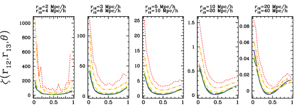
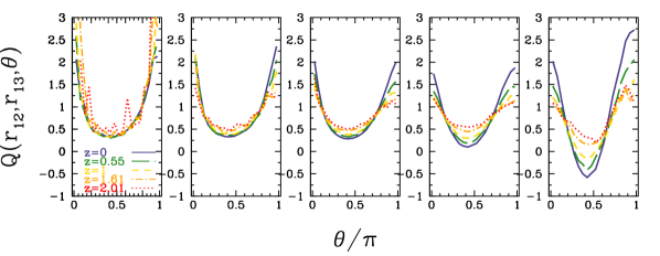
Figure 1 shows the 3PCF $\zeta(\theta)$ (upper panels) and $Q(\theta)$ (lower panels), as a function of redshift and scale, as indicated by the labels. Here we show only the $\Lambda$CDM results, since the trends we are about to discuss are similar in the different models. The main results of this first analysis can be summarised as follows:

1. at each scale and redshift, the reduced 3PCF $Q$ is higher for elongated triangles than for perpendicular ones. This is a well understood effect (Gaztañaga & Scoccimarro, 2005; Marín et al., 2008), due to the fact that cosmic structures preferentially move along gradients of the density field within non-linear gravitational instabilities (Bernardeau et al., 2002);

2. at fixed scale, we find a clear redshift trend in both $\zeta$ and $Q$: the halo 3PCF increases going to high redshift, while the reduced 3PCF becomes flatter. The former result simply reflects the evolution of the bias function in mass-selected samples (see also §4.4), while the evolution of the reduced 3PCF can be interpreted as the imprint of the formation of filaments along the cosmic time. Indeed, this trend is more evident at large scales, with differences up to $\Delta Q\sim 1$ between $z\sim 0$ and $z\sim 2$ We also notice that the difference of $Q$ between elongated and perpendicular configurations increases with decreasing redshift;

3. at fixed redshift, the reduced 3PCF exhibits a transition from a U-shape, at small scales, to a V-shape, at large scales, consistently with previous results from numerical investigations (see Gaztañaga & Scoccimarro, 2005; Marín et al., 2008). This is a consequence of the fact that, at small scales, structures reside preferentially in rounder structures (hence $Q$ is flatter), while at larger scales the contribution of structures in filaments starts becoming important.

4.3 Impact of different cosmological models

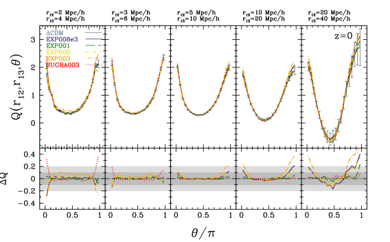
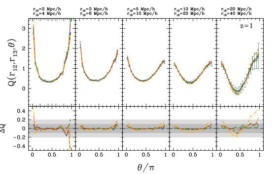
As a next step, we compare the 3PCF of different cosmological models, at fixed scale and redshift. The result is shown in Figs. 2 and 3 at redshifts $z=0$ and $z=1$ (respectively), as examples. In the lower panel of each plot we show the difference, $\Delta Q$, between the values of $Q$ of each cosmological model and the $\Lambda$CDM ones. The errorbars are estimated from the scatter among the 3PCF measured in sub-volumes of a larger simulation. Specifically, we used the CDM sub-halo catalogues extracted from the new XL-CoDECS simulations, generated with the same pipeline described in §2, but in a larger volume of $(2h^{-1}\,\mbox{Gpc})^{3}$. We divided each snapshot of the $\Lambda$CDM XL-CoDECS simulation into $27$ sub-cubes, and used them to estimate the full normalised covariance matrix of our measurements. Each sub-cube is $\sim 700$ $h^{-1}\,\mbox{Mpc}$ on a side, so its volume is comparable to the one of the L-CoDECS simulations. The errorbars shown in Figs. 2 and 3 are the r.m.s. between the 3PCF measured in these sub-cubes, i.e. the square root of the diagonal elements of the covariance matrix. More details can be found in Appendix A.

Figure 5: The bias estimated from the 3PCF in the $\Lambda$CDM simulation at $z=1$. The reduced 3PCF of DM (dashed lines) and haloes (points with errorbars) is shown at different scales $\{r_{12},r_{13}\}=\{5,10\},\{10,20\},\{20,40\}$ $h^{-1}\,\mbox{Mpc}$ , from left to right. The long-dashed red lines and the solid blue lines show the best-fit values of $Q(\theta)$ obtained with Eq. 10 from a fit to each single scale and from a joint analysis, respectively.

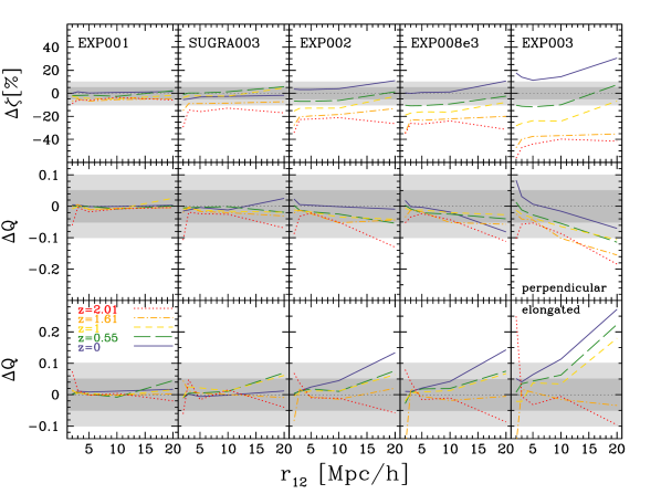
In Fig. 4 we report the mean fractional differences in percent in $\zeta$ (upper panels) and the mean differences $\Delta Q$ for perpendicular (intermediate panels) and elongated configurations (lower panels), between cDE and $\Lambda$CDM predictions. The latter quantities are obtained by averaging the differences at each scale over the angle $\theta$, and are reported as a function of the length of the first side of the triangles, $r_{1}$. We verified that the differences in $\zeta$ do not vary significantly as a function of the angle, presenting a shift that is almost constant as a function of scale. Therefore, we decided to average those differences over the full range $0\leq\theta\leq\pi$. On the other hand, being normalised over the 2PCF, the differences in $Q$ averaged over the entire angle range present an almost null shift, while the angular dependence is more significant. Hence, we considered the cases of perpendicular and elongated configurations separately, averaging the values of $\Delta Q$ in the ranges $0.3<\theta/\pi<0.7$ and $\theta/\pi\leq 0.3\;\cup\;\theta/\pi\geq 0.7$, respectively. For illustrative purpose, in Tab. 2 we reported the mean fractional differences for the EXP003 model at $z=1$.

Table 2: Mean fractional differences in percent $\Delta\zeta[\%]$ and mean differences $\Delta Q$ for EXP003 model at $z=1$.

scale	$\Delta\zeta[\%]$	$\Delta Q$	$\Delta Q$
$\rm[h^{-1}Mpc]$		perpendicular	elongated
2-4	7.5	-0.01	-0.02
3-6	-28	-0.02	-0.02
5-10	-26	-0.04	0.04
10-20	-23.8	-0.06	0.03
20-40	-6.8	-0.11	0.18

The most interesting findings shown in Figs. 2 and 3 and 4 can be summarised as follows:

1. at fixed redshift, we find significant differences between the halo 3PCF of cDE and $\Lambda$CDM simulations, that become more and more evident at increasing scales;

2. cDE models display a higher (lower) reduced 3PCF, with respect to the $\Lambda$CDM scenario, for elongated (perpendicular) configurations;

3. at fixed scale, the differences are larger for elongated configurations;

4. the differences increase with redshift, being almost negligible at $z=0$.

While the differences between the $\zeta$ values in $\Lambda$CDM and cDE simulations are independent of the considered scale, there is a strong shape dependence in $\Delta Q$, which presents opposite trends as a function of the configuration: cDE cosmologies have always a smaller (larger) 3PCF than $\Lambda$CDM for perpendicular (elongated) triangles. The differences in $\zeta$ between cDE and $\Lambda$CDM simulations are in line with the 2PCF measurements by MBM12.

We conclude that both the normalisation and the shape of the 3PCF of cDE models are different from the $\Lambda$CDM ones, and can be used to discriminate among models. Only the EXP001 model appears almost indistinguishable from $\Lambda$CDM in terms of the 3PCF, in the whole range of redshifts and scales considered. The model that deviates the most from the $\Lambda$CDM cosmology is EXP003, with differences up to $\sim 50\%$ in $\zeta$, at $z\sim 2$.

4.4 From the 3PCF to the halo bias

Figure 6: Contour plot of $b_{1}$ and $b_{2}/b_{1}$ estimated at $z=1$ from the joint analysis presented in Fig. 5. Light and dark shaded area represent the 68% and 95% confidence levels. The vertical line indicates the value of $b_{1}$ estimated with Eq. 9, while the red shaded area is the associated $1\,\sigma$ uncertainty.

From the measured 2PCF of a given sample of astrophysical sources it is possible to infer their bias function with respect to the underlying DM distribution. Using a Taylor expansion of the halo biasing function to the second order (Fry & Gaztanaga, 1993), the halo overdensity, $\delta_{\rm h}$, can be expressed, at large scales, as a function of the DM overdensity, $\delta_{\rm DM}$, as follows:

$$\delta_{\rm h}\approx b_{1}\delta_{\rm DM}+\frac{b_{2}}{2}\delta^{2}_{\rm DM}\,,$$ (8)

where $b_{1}$ and $b_{2}$ are two bias factors. From Eq. 8, we can derive a simple relation between the halo 2PCF and the linear halo bias:

$$\xi_{\rm h}(r)\approx b_{1}^{2}\xi_{\rm DM}(r)\,,$$ (9)

where $\xi_{\rm DM}$ and $\xi_{\rm h}$ are the 2PCF of DM and haloes, respectively. A similar relation can be derived also for the 3PCF:

$$Q_{\rm h}(\theta)\approx\frac{1}{b_{1}}\left(Q_{\rm DM}(\theta)+\frac{b_{2}}{b_{1}}\right)\,,$$ (10)

where $Q_{\rm DM}$ and $Q_{\rm h}$ are the reduced 3PCF of DM and haloes, respectively.

Figure 7: Bias of CDM haloes estimated from the 3PCF (Eq. 10) in three different cosmological models. Upper panels: the coloured lines show the best-fit values obtained for $r_{12}=5,10,20$ $h^{-1}\,\mbox{Mpc}$ and $r_{13}=2r_{12}$, and by combining together all the scales (yellow, green and blue lines, and black dots, respectively). Open red dots show the bias as estimated from the 2PCF (Eq. 9) in the range $10<r[$$h^{-1}\,\mbox{Mpc}$ $]<50$. The dashed and dotted lines display the theoretical effective bias as predicted by Sheth et al. (2001) and Tinker et al. (2010), with the grey shaded areas showing a $10\%$ error, representative of theoretical uncertainties. Lower panels: fractional difference in percent between the bias estimated from 3PCF and 2PCF, defined as $\Delta b/b_{2PCF}[\%]=(b_{3PCF}-b_{2PCF})/b_{2PCF}\cdot 100$. The coloured lines are the same as in the upper panels. The light and dark shaded areas represent the 25% and 50% levels. The points have been slightly shifted along the horizontal axis to make the figure clearer.

Different cosmological models predict different values for $b_{1}$ and $b_{2}/b_{1}$, and a distinct redshift evolution. Therefore, the halo bias can be a powerful probe to discriminate between alternative cosmological scenarios. In particular, it can be shown that the bias in cDE models is significantly different than the one predicted by the $\Lambda$CDM scenario (see e.g. MBM12).

However, two key issues arise when analysing real datasets. Firstly, the halo bias has to be inferred from the measured galaxy bias, that depends not trivially on both baryon phenomena and selection effects. Secondly, if the bias is estimated from the 2PCF, i.e. using Eq. 9, a fiducial value of $\sigma_{8}$ has to be assumed to compute $\xi_{\rm DM}$. Since $\xi_{\rm DM}\propto\sigma_{8}^{2}$ at large scales, the bias amplitude scales approximately as $\sigma_{8}^{-1}$ in the linear regime. MBM12 found that the suppression of the halo bias caused by the DE coupling is degenerate with $\sigma_{8}$ at scales $r\gtrsim 5$ $h^{-1}\,\mbox{Mpc}$ , i.e. the different halo biases of cDE cosmologies may be simply recovered with a $\Lambda$CDM model with a rescaled value of $\sigma_{8}$. Therefore, without any prior on $\sigma_{8}$, it is impossible to detect any signature of DE coupling using only the 2PCF at large scales.

The same considerations hold for the 3PCF as well, since it can be shown that the matter 3PCF, $\zeta_{\rm DM}$, scales as $\sigma_{8}^{4}$ (Pan & Szapudi, 2005). On the contrary, the reduced 3PCF $Q\sim\zeta/\xi^{2}$ does not depend on $\sigma_{8}$ by construction, so that the bias factors estimated with Eq. 10 do not require any prior on $\sigma_{8}$.

To derive the bias factors $b_{1}$ and $b_{2}/b_{1}$ of Eq. 10, we apply a standard $\chi^{2}$ minimization approach using only the diagonal elements of the covariance matrix, i.e. minimizing the function:

$$\chi^{2}=\sum\frac{(Q_{\rm h}-Q_{\rm h}^{\rm model})^{2}}{\sigma_{Q}^{2}}\,,$$ (11)

where the errors $\sigma_{Q}$ have been estimated as discussed in §4.1, and $Q_{\rm h}$ and $Q_{\rm h}^{\rm model}$ are the measured and theoretical reduced 3PCFs, respectively, the latter quantity being given by Eq. 10, where the CDM reduced 3PCF $Q_{\rm DM}$ is estimated using sparsely sampled sub-sets of the CDM particle snapshots, to decrease the computational time. The uncertainties estimated through Eq. 11 are slightly underestimated, not taking into account the full covariance between measurements in different bins, as discussed in Appendix A, where we also discuss the impact of considering the full covariance matrix in the analysis. However, for the purpose of this work this is not relevant: all the CoDECS simulations match the same cosmology at $z_{\rm CMB}$ by construction, so the differences between the reduced 3PCF measured in these catalogues are real differences. The aim of showing uncertainties in the bias factors is just to give a qualitative feeling on the expected uncertainties in surveys comparable to the CoDECS samples in terms of volume and density of objects.

Equations 9 and 10 are reliable approximations of the halo clustering only at large, linear scales. Therefore, we use them to derive the halo bias at our three largest configurations, in which triangles have sides $\{r_{12},r_{13}\}=\{5,10\},\{10,20\},\{20,40\}$ $h^{-1}\,\mbox{Mpc}$ , respectively. Different scales have been examined both separately and jointly.

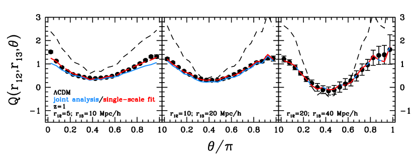
As an illustrative case, we show the result of the analysis for the $\Lambda$CDM model at $z=1$. In Fig. 5 is presented the reduced 3PCF of CDM (dotted lines) and haloes (points with errorbars) at the different scales. Red and blue lines display the best-fit models for the reduced 3PCF of haloes, obtained from Eqs. 10 considering each scale separately and with a joint analysis, respectively. The best fit obtained by fixing the bias with the 2PCF from Eq. 9 is not shown, since it perfectly overlaps with the fit obtained with the 3PCF joint analysis. In this case, the $b_{2}$ parameter has been obtained by minimizing the $\chi^{2}$, having fixed the bias $b_{1}$. The complete agreement between the latter, at all scales, demonstrates that the linear halo bias factors derived from the 2PCF and from the 3PCF are equivalent, at least at the redshifts and scales considered here. In summary, Fig. 5 shows that the method to derive the halo bias from the 3PCF is reliable at $z=1$ and at the scales considered here. As already noted before, the crucial advantage of using the reduced 3PCF $Q(\theta)$ is that it does not depend on $\sigma_{8}$, differently from the 2PCF and the 3PCF $\zeta(\theta)$.
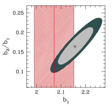
This can also be appreciated in Fig. 6. It shows the bias parameters $b_{1}$ and $b_{2}/b_{1}$, estimated from the 3PCF (grey contours), compared to the parameter $b_{1}$, estimated from the 2PCF (red vertical line). Specifically, the light and grey contour plots are the $68$ and $95$ per cent likelihood probability contours in the $b_{1}-b_{2}/b_{1}$ planes, obtained with Eqs. 10 and 11 and combining together the measurements at the three scales considered here.

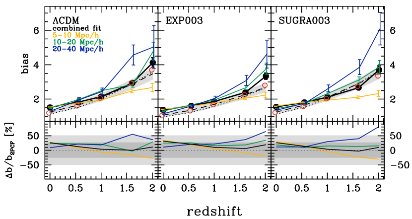
Figure 7 extends the previous analysis, showing the halo bias in the redshift range $0\leq z\leq 2$ and comparing the $\Lambda$CDM case with the EXP003 and SUGRA003 simulations, as indicated by the labels. Among the cDE models of the CoDECS simulations, EXP003 and SUGRA003 are the ones that differ the most from the $\Lambda$CDM case. Coloured and black lines show the results obtained with separate and joint scales, respectively. These estimates are compared with both the biases obtained from the 2PCF (through Eq. 9), in the range $10<r<50$ $h^{-1}\,\mbox{Mpc}$ , and with the theoretical $\Lambda$CDM effective bias values predicted by Sheth et al. (2001) and Tinker et al. (2010), normalised to the $\sigma_{8}$ values of each respective model, and weighted by the halo mass function, as in MBM12 (see their Fig.2 and related discussion). The shaded areas show a representative $10\%$ scatter, that reflects the uncertainty in the theoretical predictions, as found in the literature (e.g. see the differences between Sheth & Tormen, 1999; Sheth et al., 2001; Tinker et al., 2010). In the lower panels of Fig. 7, we show the fractional difference in percent of the bias as estimated from the 3PCF with respect to the bias estimated from the 2PCF, i.e. $\Delta b/b_{2PCF}[\%]=(b_{3PCF}-b_{2PCF})/b_{2PCF}\cdot 100$.

While the linear bias obtained from the 2PCF results in excellent agreement with theoretical predictions, at all redshifts and for all the cDE models considered, as already noted by MBM12, the goodness of the bias derived from the 3PCF depends on the scales used. In particular, the agreement is better when the bias is estimated from the reduced 3PCF measured at the largest scales ($r_{12}\geq 10$ $h^{-1}\,\mbox{Mpc}$ ), as expected since the linear bias model given by Eq. 10 is a good approximation only in the linear regime ($r\gtrsim 10$ $h^{-1}\,\mbox{Mpc}$ ). On the other hand, the larger discrepancies at higher redshift are due to the sparseness of DM samples used to estimate $Q_{\rm DM}$ in Eq. 10. A more detailed analysis using theoretical predictions for $Q_{\rm DM}$ is deferred to a future paper.

Figure 7 shows that the bias estimated from the combination of the reduced 3PCF measured at all three scales considered better reproduces the real bias of our simulations, even though in this analysis we do not take into account the covariance between different scales (see discussion in Appendix A). We note, however, that at high redshift this is just a spurious effect, caused by the compensation of the underestimation of the bias at small scales and the overestimation at large scales.

As already noted in Fig. 5, the bias estimated from the 3PCF appears in reasonable agreement with the true one at $z=1$, especially when assessed from the combination of scales. Moreover, Fig. 7 shows that this is true also for the models EXP003 and SUGRA003. On the other hand, the agreement is worst at both lower and higher redshifts. In particular, similarly as previous findings by Marín et al. (2008), our analysis shows that the bias estimated from Eq. 10 slightly overestimates the one given by Eq. 9 by $\sim 15-25\%$, on average, as can be seen in the lower panels of Fig. 7. However, we point out that the significance of such a discrepancy, that in many cases is below the $1\,\sigma$ estimated uncertainty, may be further reduced when considering also the error on the bias estimate from the 2PCF, typically of the order of 5-10 $\%$ (e.g. see the red shaded area of Fig. 6). These discrepancies become smaller, of the order of $\sim 10-20\%$, and similar to the ones quoted by Marín et al. (2008), when considering the analysis at combined scales. Our results are also in agreement with the work by Hoffmann et al. (2014). They analysed the MICE-GC $\Lambda$CDM simulation with a method similar to the one adopted in this paper, finding that the linear bias estimated from the 3PCF $Q$ overestimates the one from the 2PCF by $\sim$30-40%, at all mass and redshift ranges considered. Our work extends these findings to cDE cosmologies.

Overall, these systematics indicate that assuming a local deterministic bias model can significantly affect the results, and that further developments from the theoretical side are required.

Figure 8: Bias of CDM haloes estimated from the 3PCF, using different cosmological models to compute $Q_{\rm h}$ and $Q_{\rm DM}$. In particular, $Q_{\rm h}$ is measured in the EXP003 simulation, while $Q_{\rm DM}$ in the $\Lambda$CDM one. As a comparison, we also reported the bias function obtained with the correct cosmology (dashed coloured lines) and theoretical predictions (dotted and dashed lines). The symbols of the latter quantities are the same as in Fig. 7. The points have been slightly shifted along the horizontal axis to make the figure clearer.

4.5 Geometric distortions

In the previous section we demonstrated that the 3PCF can be used to estimate the halo bias in a $\sigma_{8}$-independent way. All the measurements discussed so far assumed the correct underlying cosmology when estimating both the CDM and the halo correlation functions, i.e. we always employed cosmic distances that were numerically computed according to each cosmological model under investigation. However, when analysing real datasets, the true cosmology of the Universe is unknown.

If a wrong cosmology is assumed when converting redshifts into comoving distances, the measured 2PCF and 3PCF will be distorted. As discussed in MBM12, this geometric effect is small for the cDE models analysed in this work, since they are nearly indistinguishable in terms of the Hubble function. Besides this effect on measured quantities, a wrong assumption on the underlying cosmology impacts also the function $Q_{\rm DM}(\theta)$ used in Eq. 10. The latter is generally estimated using standard $\Lambda$CDM simulations, with fixed cosmological parameters (see e.g. Gaztañaga et al., 2005; Ross et al., 2006; McBride et al., 2011a, b; Marín, 2011; Marín et al., 2013). At the present state, no attempt has been done to investigate the impact of assuming a wrong cosmology when estimating $Q_{\rm DM}(\theta)$, especially in non-standard cosmological scenarios.

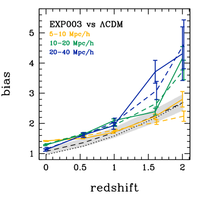
In the following, we test this effect in the case of cDE models using our CoDECS datasets. Specifically, we investigate the effect of measuring the bias from Eq. 10 assuming different models for $Q_{\rm h}$ and $Q_{\rm DM}$. To maximise the effect, we consider the $\Lambda$CDM and EXP003 cosmologies, since the latter is the model that differs the most from the $\Lambda$CDM case. Fig. 8 displays the results of this test. In this figure, we show the bias of CDM haloes estimated using the function $Q_{\rm h}(\theta)$ measured in the EXP003 simulations, while $Q_{\rm DM}(\theta)$ is measured in the $\Lambda$CDM ones. This case represents the hypothetical situation in which an observer living in a (quite extreme) cDE universe attempts to estimate the bias assuming a $\Lambda$CDM model to compute $Q_{\rm DM}(\theta)$. As it can be seen, the bias functions obtained with (dashed lines) and without (solid lines) assuming the correct cosmology for the DM 3PCF are consistent, considering the quoted errorbars, for all the scales and redshift analysed, with no particular systematic trend. This is a quite remarkable result: the determination of the bias through the 3PCF seems to be mostly independent of the cosmological model, even for rather complex and extreme extensions beyond the standard $\Lambda$CDM scenario.

5 Conclusions

In this work we investigated the power of the 3PCF to constrain cDE models, and to estimate the halo bias in these cosmological scenarios. We analysed halo catalogues extracted from the CoDECS simulations, which are large, collisionless N-body simulations of a variety of cosmological models in which the DE scalar field can interact with CDM particles by exchanging energy-momentum. We estimated the 3PCF $\zeta(\theta)$ and the reduced 3PCF $Q(\theta)$ for triplets of objects in which $r_{12}/r_{13}=2$, where $r_{12}$ and $r_{13}$ are the comoving separations between two of the objects, and $\theta$ is the angle between them. We considered different representative scales ($r_{12}=2,3,5,10,20$ $h^{-1}\,\mbox{Mpc}$ ) and redshifts ($z=0,0.55,1,1.61,2.01$).

The main results of this analysis, independently of the cosmological model considered, are as follows:

• at both fixed scale and redshift, the reduced 3PCF is higher for elongated triangles than for perpendicular ones, as expected from non-linear gravitational instability theory;

• at fixed scale, the 3PCF increases going to higher redshift, while the reduced 3PCF becomes flatter, which is a signature of the evolution of the bias function and of the formation of filaments with cosmic time;

• at fixed redshift, we see a transition in the reduced 3PCF from a U-shape, at small scales, to a V-shape, at large scales. This is a consequence of the fact that, at small scales, structures preferentially reside in approximately round structures (hence presenting a flatter $Q$), while at larger scales also the contribution of structures in filaments starts to become significant.

Overall, these results confirm what already found in the literature at $z\sim 0$ (e.q. Gaztañaga & Scoccimarro, 2005; Marín et al., 2008), and extend it to a wider redshift range and different cosmologies.

Regarding the effects of DE coupling on the halo 3PCF, our main results are as follows:

• the 3PCF in cDE models is significantly different than in the $\Lambda$CDM scenario, with deviations that increase going to larger scales;

• at fixed scale, cDE models predict a higher (smaller) 3PCF for elongated (perpendicular) configurations with respect to the $\Lambda$CDM cosmology;

• the differences increase with redshift, being almost negligible at $z=0$.

These 3PCF measurements have been used to constrain the linear bias function of CDM haloes in the redshift range $0\leq z\leq 2$. We considered three configuration scales ($s=5,10,20$ $h^{-1}\,\mbox{Mpc}$ ), both separately and with a joint analysis. We find a reasonable agreement, considering the estimated uncertainties, between the bias estimated from the 3PCF and from the 2PCF. However, we also find that the 3PCF tends to systematically overestimate the bias by $\sim$15-25% on average, mainly due to the linear approximations in the theoretical modelisation. These results are in good agreement with the works of Marín et al. (2008) and Hoffmann et al. (2014), for the $\Lambda$CDM case. Finally, we quantified the impact of assuming a wrong cosmology in estimating the halo bias, using different cosmologies for the reduced 3PCF of DM and haloes. Even in the most extreme case analysed in this work, we find that this effect is negligible considering the uncertainties.

This work demonstrates that the 3PCF can be efficiently exploited, as a complementary probe to lower-order statistics, to discriminate between alternative cosmological scenarios. In particular, we proved that the degeneracy between the halo bias and $\sigma_{8}$ can be broken using the reduced 3PCF $Q(\theta)$. Moreover, combining measurements of redshift-space distortions in the 2PCF with $\sigma_{8}$ constraints from the reduced 3PCF, it will be possible to estimate directly the growth rate of structures $f(z)$.

The differences found between the various models are indeed small, and the errors on the bias provided by present surveys are just of the order of these differences, not yet allowing to disentangle between standard and alternative cosmologies (e.g., see Marín et al., 2013). However, ongoing and future surveys, such as BOSS (Schlegel et al., 2009), WiggleZ (Blake et al., 2011b), VIPERS (Guzzo et al., 2014), and Euclid (Laureijs et al., 2011), will be able to increase current statistics by more than one order of magnitude, reducing dramatically the expected statistical errors, though a more detailed assessment of the theoretical framework is required to understand the systematics highlighted in this work. In this context, the analysis of the 3PCF will be of extreme importance also at the BAO scale, as recently shown by Fosalba et al. (2013) and Crocce et al. (2013).

Appendix A Covariance matrices

Figure 9: Normalised covariance matrices estimated with the large $\Lambda$CDM simulation of the new XL-CoDECS series ($2\times 2048^{3}$ particles over a $2$ $h^{-1}\,\mbox{Gpc}$ periodic cosmological box), at all scales (from lower to upper panels) and redshifts (from left to right) considered in this work. The redshift range is labeled above the upper panels, while at the right can be found the scale considerend.

Figure 10: Normalised covariance matrices between mixed scales, at redshifts $z=0$ (left panel), $z=1$ (right panel). The diagonal squares presents just the normalised covariance matrix of every single scale, as shown in Fig. 9, while the off-diagonal squares present the normalised covariance matrix between different scales; the corresponding scale can be found labeled above and at the right of each panel.

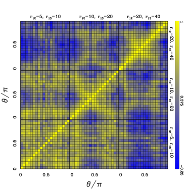
The covariance matrices used in this paper to estimate the errors on $\zeta(\theta)$ and $Q(\theta)$ are derived using the large XL-CoDECS $\Lambda$CDM simulation. As explained in §4.1, we divided the CoDECS-XL snapshots into $N=27$ sub-cubes of side $\sim 700$ $h^{-1}\,\mbox{Mpc}$ . The normalised covariance matrix is defined as follows:

$$C_{ij}=\frac{1}{N}\sum_{k=1}^{N}\left(\frac{Q_{i}^{k}-\bar{Q}_{i}}{\sigma_{Q_{i}}}\right)\left(\frac{Q_{j}^{k}-\bar{Q}_{j}}{\sigma_{Q_{j}}}\right)\,,$$ (12)

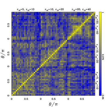
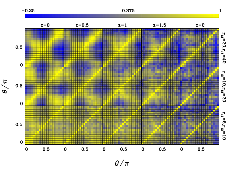
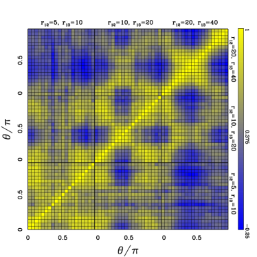
where $\bar{Q}_{j}$ is the mean value of the reduced 3PCF in the $N$ sub-cubes. Fig. 9 shows the normalised covariance matrices at all the redshifts and scales considered in this analysis, i.e. $0\leq z\leq 2$, $s=2$ $h^{-1}\,\mbox{Mpc}$ and $u=5,10,20$ $h^{-1}\,\mbox{Mpc}$ . We find a significant covariance between different bins, especially at small angles and scales. At high redshifts and large scales, the covariance matrices become gradually more and more diagonal. Qualitatively, these results are in good agreement with the covariance matrices found for similar configurations by Gaztañaga & Scoccimarro (2005) and Hoffmann et al. (2014). To perform the joint analysis discussed in §4.5, we also estimated the covariance matrix between different scales. The result is shown in Figs. 10 and 11, for three characteristic redshifts. At high redshift, the covariance between different scales is quite small, and the matrix is almost diagonal. The correlations between scales increases with decreasing redshift.

To derive the bias parameters of Eq. 10, we performed a full-covariance $\chi^{2}$ analysis, with:

$$\chi^{2}=\sum_{i=1}^{N}\sum_{j=1}^{N}\left(\frac{Q_{i}(\theta)-Q^{\rm model}_{i}(\theta)}{\sigma_{Q_{i}(\theta)}}\right)C_{ij}^{-1}\left(\frac{Q_{j}(\theta)-Q^{\rm model}_{j}(\theta)}{\sigma_{Q_{j}(\theta)}}\right)\,.$$ (13)

However, in most cases the limited number of available sub-mocks introduces numerical instabilities in the inversion of $C_{ij}$, biasing the final results. For this reason we decided to use only the diagonal elements of the covariance matrix in our computations (see Eq. 11). For a small subset of cases where this issue was less severe, we verified that the difference in the bias parameter estimation is of the order of 0.1, and the difference in the estimated error of the order of 0.015. A similar analysis of the impact of the covariance matrix on the bias estimate has been carried out also by Hoffmann et al. (2014), reaching a similar conclusion that the results are not strongly dependent on the uncertainty in the covariance matrix.

Moreover, by looking at Fig. 9, we see that the impact of this assumption is most severe at low redshifts and at small scales. On the contrary, at large scales and redshifts the off-diagonal terms are small, and can be safely neglected.

Figure 11: Normalised covariance matrices between mixed scales, at redshift $z=2$. The labels are the same as Fig. 10

References

- Amendola (2000) Amendola L., 2000, Phys. Rev. D, 62, 043511
- Amendola et al. (2013) Amendola L., et al., 2013, Living Reviews in Relativity, 16, 6
- Anderson et al. (2012) Anderson L., et al., 2012, Mon. Not. R. Astron. Soc., 427, 3435
- Baldi (2011a) Baldi M., 2011a, Mon. Not. R. Astron. Soc., 414, 116
- Baldi (2011b) —, 2011b, Mon. Not. R. Astron. Soc., 411, 1077
- Baldi (2012a) —, 2012a, Mon. Not. R. Astron. Soc., 420, 430
- Baldi (2012b) —, 2012b, Mon. Not. R. Astron. Soc., 422, 1028
- Baldi et al. (2014) Baldi M., Villaescusa-Navarro F., Viel M., Puchwein E., Springel V., Moscardini L., 2014, Mon. Not. R. Astron. Soc., 440, 75
- Bernardeau et al. (2002) Bernardeau F., Colombi S., Gaztañaga E., Scoccimarro R., 2002, Phys. Rept., 367, 1
- Beutler et al. (2011) Beutler F., et al., 2011, Mon. Not. R. Astron. Soc., 416, 3017
- Blake et al. (2011a) Blake C., et al., 2011a, Mon. Not. R. Astron. Soc., 418, 1707
- Blake et al. (2011b) —, 2011b, Mon. Not. R. Astron. Soc., 418, 1725
- Brax & Martin (1999) Brax P. H., Martin J., 1999, Physics Letters B, 468, 40
- Cabré & Gaztañaga (2009) Cabré A., Gaztañaga E., 2009, Mon. Not. R. Astron. Soc., 396, 1119
- Chuang & Wang (2012) Chuang C.-H., Wang Y., 2012, Mon. Not. R. Astron. Soc., 426, 226
- Cole et al. (2005) Cole S., et al., 2005, Mon. Not. R. Astron. Soc., 362, 505
- Crocce et al. (2013) Crocce M., Castander F. J., Gaztanaga E., Fosalba P., Carretero J., 2013, ArXiv:1312.2013
- da Ângela et al. (2005) da Ângela J., Outram P. J., Shanks T., 2005, Mon. Not. R. Astron. Soc., 361, 879
- Damour et al. (1990) Damour T., Gibbons G. W., Gundlach C., 1990, Phys. Rev. Lett., 64, 123
- Davis et al. (1985) Davis M., Efstathiou G., Frenk C. S., White S. D. M., 1985, Astrophys. J., 292, 371
- de la Torre et al. (2013) de la Torre S., et al., 2013, Astron. Astrophys., 557, A54
- Eisenstein et al. (2005) Eisenstein D. J., et al., 2005, Astrophys. J., 633, 560
- Fosalba et al. (2013) Fosalba P., Crocce M., Gaztanaga E., Castander F. J., 2013, ArXiv:1312.1707
- Frieman & Gaztanaga (1994) Frieman J. A., Gaztanaga E., 1994, Astrophys. J., 425, 392
- Fry (1994) Fry J. N., 1994, Physical Review Letters, 73, 215
- Fry & Gaztanaga (1993) Fry J. N., Gaztanaga E., 1993, Astrophys. J., 413, 447
- Fry & Seldner (1982) Fry J. N., Seldner M., 1982, Astrophys. J., 259, 474
- Garilli et al. (2014) Garilli B., et al., 2014, Astron. Astrophys., 562, A23
- Gaztañaga et al. (2005) Gaztañaga E., Norberg P., Baugh C. M., Croton D. J., 2005, Mon. Not. R. Astron. Soc., 364, 620
- Gaztañaga & Scoccimarro (2005) Gaztañaga E., Scoccimarro R., 2005, Mon. Not. R. Astron. Soc., 361, 824
- Guo et al. (2014) Guo H., Li C., Jing Y. P., Börner G., 2014, Astrophys. J., 780, 139
- Guzzo et al. (2008) Guzzo L., et al., 2008, Nature, 451, 541
- Guzzo et al. (2014) —, 2014, Astron. Astrophys., 566, A108
- Hawkins et al. (2003) Hawkins E., et al., 2003, Mon. Not. R. Astron. Soc., 346, 78
- Hoffmann et al. (2014) Hoffmann K., Bel J., Gaztanaga E., Crocce M., Fosalba P., Castander F. J., 2014, arXiv:1403.1259
- Jing & Boerner (1997) Jing Y. P., Boerner G., 1997, Astron. Astrophys., 318, 667
- Jing & Börner (2004) Jing Y. P., Börner G., 2004, Astrophys. J., 607, 140
- Kayo et al. (2004) Kayo I., et al., 2004, Publ. Astron. Soc. Japan, 56, 415
- Kazin et al. (2010) Kazin E. A., et al., 2010, Astrophys. J., 710, 1444
- Komatsu et al. (2011) Komatsu E., et al., 2011, Astrophys. J. Suppl., 192, 18
- Kulkarni et al. (2007) Kulkarni G. V., Nichol R. C., Sheth R. K., Seo H.-J., Eisenstein D. J., Gray A., 2007, Mon. Not. R. Astron. Soc., 378, 1196
- Landy & Szalay (1993) Landy S. D., Szalay A. S., 1993, Astrophys. J., 412, 64
- Laureijs et al. (2011) Laureijs R., et al., 2011, arXiv:1110.3193
- Lucchin & Matarrese (1985) Lucchin F., Matarrese S., 1985, Phys. Rev. D, 32, 1316
- Marín (2011) Marín F., 2011, Astrophys. J., 737, 97
- Marín et al. (2008) Marín F. A., Wechsler R. H., Frieman J. A., Nichol R. C., 2008, Astrophys. J., 672, 849
- Marín et al. (2013) Marín F. A., et al., 2013, Mon. Not. R. Astron. Soc., 432, 2654
- Marulli et al. (2012a) Marulli F., Baldi M., Moscardini L., 2012a, Mon. Not. R. Astron. Soc., 420, 2377
- Marulli et al. (2012b) Marulli F., Bianchi D., Branchini E., Guzzo L., Moscardini L., Angulo R. E., 2012b, Mon. Not. R. Astron. Soc., 426, 2566
- Marulli et al. (2011) Marulli F., Carbone C., Viel M., Moscardini L., Cimatti A., 2011, Mon. Not. R. Astron. Soc., 418, 346
- Marulli et al. (2013) Marulli F., et al., 2013, Astron. Astrophys., 557, A17
- Matarrese et al. (1997) Matarrese S., Verde L., Heavens A. F., 1997, Mon. Not. R. Astron. Soc., 290, 651
- McBride et al. (2011a) McBride C. K., Connolly A. J., Gardner J. P., Scranton R., Newman J. A., Scoccimarro R., Zehavi I., Schneider D. P., 2011a, Astrophys. J., 726, 13
- McBride et al. (2011b) McBride C. K., Connolly A. J., Gardner J. P., Scranton R., Scoccimarro R., Berlind A. A., Marín F., Schneider D. P., 2011b, Astrophys. J., 739, 85
- Nichol et al. (2006) Nichol R. C., et al., 2006, Mon. Not. R. Astron. Soc., 368, 1507
- Padmanabhan et al. (2012) Padmanabhan N., et al., 2012, Mon. Not. R. Astron. Soc., 427, 2132
- Pan & Szapudi (2005) Pan J., Szapudi I., 2005, Mon. Not. R. Astron. Soc., 362, 1363
- Peebles (1980) Peebles P. J. E., 1980, The Large-Scale Structure of the Universe, Princeton University Press
- Peebles & Groth (1975) Peebles P. J. E., Groth E. J., 1975, Astrophys. J., 196, 1
- Percival et al. (2007) Percival W. J., Cole S., Eisenstein D. J., Nichol R. C., Peacock J. A., Pope A. C., Szalay A. S., 2007, Mon. Not. R. Astron. Soc., 381, 1053
- Percival et al. (2010) Percival W. J., et al., 2010, Mon. Not. R. Astron. Soc., 401, 2148
- Pettorino (2013) Pettorino V., 2013, Phys. Rev. D 88,, 063519
- Ross et al. (2006) Ross A. J., Brunner R. J., Myers A. D., 2006, Astrophys. J., 649, 48
- Ross et al. (2007) Ross N. P., et al., 2007, Mon. Not. R. Astron. Soc., 381, 573
- Samushia et al. (2012) Samushia L., Percival W. J., Raccanelli A., 2012, Mon. Not. R. Astron. Soc., 420, 2102
- Sánchez et al. (2009) Sánchez A. G., Crocce M., Cabré A., Baugh C. M., Gaztañaga E., 2009, Mon. Not. R. Astron. Soc., 400, 1643
- Sánchez et al. (2012) Sánchez A. G., et al., 2012, Mon. Not. R. Astron. Soc., 425, 415
- Schlegel et al. (2009) Schlegel D., White M., Eisenstein D., 2009, in Astronomy, Vol. 2010, astro2010: The Astronomy and Astrophysics Decadal Survey, p. 314
- Scoccimarro (2000) Scoccimarro R., 2000, Astrophys. J., 544, 597
- Scoccimarro et al. (2001) Scoccimarro R., Feldman H. A., Fry J. N., Frieman J. A., 2001, Astrophys. J., 546, 652
- Sefusatti & Komatsu (2007) Sefusatti E., Komatsu E., 2007, Phys. Rev. D, 76, 083004
- Sefusatti & Scoccimarro (2005) Sefusatti E., Scoccimarro R., 2005, Phys. Rev. D, 71, 063001
- Sheth et al. (2001) Sheth R. K., Mo H. J., Tormen G., 2001, Mon. Not. R. Astron. Soc., 323, 1
- Sheth & Tormen (1999) Sheth R. K., Tormen G., 1999, Mon. Not. R. Astron. Soc., 308, 119
- Springel et al. (2001) Springel V., Yoshida N., White S. D. M., 2001, New Astronomy, 6, 79
- Szapudi & Szalay (1998) Szapudi S., Szalay A. S., 1998, Astrophys. J. Lett., 494, L41
- Tinker et al. (2010) Tinker J. L., Robertson B. E., Kravtsov A. V., Klypin A., Warren M. S., Yepes G., Gottlöber S., 2010, Astrophys. J., 724, 878
- Vera Cervantes et al. (2012) Vera Cervantes V. D., Marulli F., Moscardini L., Baldi M., Cimatti A., 2012, ArXiv:1212.0853
- Verde et al. (2000) Verde L., Heavens A. F., Matarrese S., 2000, Mon. Not. R. Astron. Soc., 318, 584
- Verde et al. (1998) Verde L., Heavens A. F., Matarrese S., Moscardini L., 1998, Mon. Not. R. Astron. Soc., 300, 747
- Veropalumbo et al. (2014) Veropalumbo A., Marulli F., Moscardini L., Moresco M., Cimatti A., 2014, Mon. Not. R. Astron. Soc., 442, 3275
- Weinberg et al. (2013) Weinberg D. H., Mortonson M. J., Eisenstein D. J., Hirata C., Riess A. G., Rozo E., 2013, Phys. Rept., 530, 87
- Wetterich (1988) Wetterich C., 1988, Nuclear Physics B, 302, 668
- Wetterich (1995) —, 1995, Astron. Astrophys., 301, 321
- Zhang et al. (2008) Zhang H., Yu H., Noh H., Zhu Z.-H., 2008, Physics Letters B, 665, 319