Low-Rank Approximations for Conditional Feedforward Computation in Deep Neural Networks

Abstract

Scalability properties of deep neural networks raise key research questions, particularly as the problems considered become larger and more challenging. This paper expands on the idea of conditional computation introduced in [2], where the nodes of a deep network are augmented by a set of gating units that determine when a node should be calculated. By factorizing the weight matrix into a low-rank approximation, an estimation of the sign of the pre-nonlinearity activation can be efficiently obtained. For networks using rectified-linear hidden units, this implies that the computation of a hidden unit with an estimated negative pre-nonlinearity can be omitted altogether, as its value will become zero when nonlinearity is applied. For sparse neural networks, this can result in considerable speed gains. Experimental results using the MNIST and SVHN data sets with a fully-connected deep neural network demonstrate the performance robustness of the proposed scheme with respect to the error introduced by the conditional computation process.

1 Introduction

In recent years, deep neural networks have redefined state-of-the-art in many application domains, notably in computer vision [11] and speech processing [14]. In order to scale to more challenging problems, however, neural networks must become larger, which implies an increase in computational resources. Shifting computation to highly parallel platforms such as GPUs has enabled the training of massive neural networks that would otherwise train too slowly on conventional CPUs. While the extremely high computational power used for the experiment performed in [12] (16,000 cores training for many days) was greatly reduced in [4] (3 servers training for many days), specialized high-performance platforms still require several machines and several days of processing time. However, there may exist more fundamental changes to the algorithms involved which can greatly assist in scaling neural networks.

Many of these state-of-the-art networks have several common properties: the use of rectified-linear activation functions in the hidden neurons, and a high level of sparsity induced by dropout regularization or a sparsity-inducing penalty term on the loss function. Given that many of the activations are effectively zero, due to the combination of sparsity and the hard thresholding of rectified linear units, a large amount of computation is wasted on calculating values that are eventually truncated to zero and provide no contribution to the network outputs or error components. Here we focus on this key observation in devising a scheme that can predict the zero-valued activations in a computationally cost-efficient manner.

2 Conditional Computation in Deep Neural Networks

2.1 Exploiting Redundancy in Deep Architectures

Figure 1: An illustration of an activation estimator. $U$ and $V$ represent the factorization of the low-rank matrix and $W$ denotes the full-rank matrix. In this case, the activation estimator recommends that only the $2^{nd}$ and the $n^{th}$ neuron be computed for layer $l+1$.

In [5], the authors made the observation that deep models tend to have a high degree of redundancy in their weight parameterization. The authors exploit this redundancy in order to train as few as 5% of the weights in a neural network while estimating the other 95% with the use of carefully constructed low-rank decompositions of the weight matrices. Such a reduction in the number of active training parameters can render optimization easier by reducing the number of variables to optimize over. Moreover, it can help address the problem of scalability by greatly reducing the communication overhead in a distributed system.

Assuming there is a considerable amount of redundancy in the weight parameterization, a similar level of redundancy is likely found in the activation patterns of individual neurons. Therefore, given an input sample, the set of redundant activations in the network may be approximated. If a sufficiently accurate approximation can be obtained using low computational resources, activations for a subset of neurons in the network’s hidden layers need not be calculated.

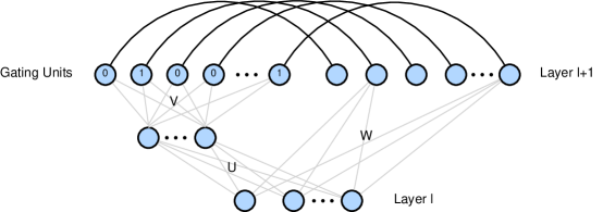
In [2] and [3], the authors propose the idea of conditional computation in neural networks, where the network is augmented by a gating model that turns activations on or off depending on the state of the network. If this gating model is able to reliably estimate which neurons need to be calculated for a particular input, great improvements in computational efficiency may be obtainable if the network is sufficiently sparse. Figure 1 illustrates a conditional computation unit augmenting a layer of a neural net by using some function $f\left(U,V,a_{l}\right)$ to determine which hidden unit activations $a_{l+1}$ should be computed given the activations $a_{l}$ of layer $l$.

2.2 Sparse Representations, Activation Functions, and Prediction

In some situations, sparse representations may be superior to dense representations, particularly in the context of deep architectures [7]. However, sparse representations learned by neural networks with sigmoidal activations are not truly “sparse”, as activations only approach zero in the limit towards negative infinity. A conditional computation model estimating the sparsity of a sigmoidal network would thus have to impose some threshold, beyond which the neuron is considered inactive. So-called “hard-threshold” activation functions such as rectified-linear units, on the other hand, produce true zeros which can be used by conditional computation models without imposing additional hyperparameters.

3 Problem Formulation

3.1 Estimating Activation Sign via Low-Rank Approximation

Figure 2: The low-rank approximation $UV$ can be substituted in for $W$, and can approximate the matrix $W$ with a relatively low rank. However, if we use the output of the activation estimator $S$, as defined in Eq. (5), with the full-rank feedforward, $\sigma\left(aW\right)\cdot S$, a lower-rank approximation can be utilized. The activations and weights are from the first layer of a neural network trained on MNIST, and the factorization $UV$ is obtained via SVD.

Given the activation $a_{l}$ of layer $l$ of a neural network, the activation $a_{l+1}$ of layer $l+1$ is given by:

$$a_{l+1}=\sigma(a_{l}W_{l})$$ (1)

where $\sigma(\cdot)$ denotes the function defining the neuron’s non-linearity, $a_{l}\in\mathbb{R}^{n\times h_{1}}$, $a_{l+1}\in\mathbb{R}^{n\times h_{2}}$, $W_{l}\in\mathbb{R}^{h_{1}\times h_{2}}$. If the weight matrix is highly redundant, as in [5], it can be well-approximated using a low-rank representation and we may rewrite (1) as

$$a_{l+1}=\sigma(a_{l}U_{l}V_{l})$$ (2)

where $U_{l}V_{l}$ is the low-rank approximation of $W_{l}$, $U_{l}\in\mathbb{R}^{h_{1}\times k}$, $V_{l}\in\mathbb{R}^{k\times h_{2}}$, $k\ll\min(h_{1},h_{2})$. So long as $k<\frac{h_{1}h_{2}}{h_{1}+h_{2}}$, the low-rank multiplication $a_{l}U_{l}V_{l}$ requires fewer arithmetic operations than the full-rank multiplication $a_{l}W_{l}$, assuming the multiplication $a_{l}U_{l}$ occurs first. When $\sigma(\cdot)$ is the rectified-linear function,

$$\sigma(x)=\max(0,x)$$ (3)

such that all negative elements of the linear transform $a_{l}W_{l}$ become zero, one only needs to estimate the sign of the elements of the linear transform in order to predict the zero-valued elements. Assuming the weights in a deep neural network can be well-approximated using a low-rank estimation, the small error in the low-rank estimation is of marginal relevance in the context of recovering the sign of the operation.

Given a low-rank approximation $W_{l}\approx U_{l}V_{l}=\hat{W}_{l}$, the estimated sign of $a_{l+1}$ is given by

$$sgn(a_{l+1})\approx sgn(a_{l}\hat{W}_{l})$$ (4)

Each element $\left(a_{l+1}\right)_{i,j}$ is given by a dot product between the row vector $a_{l}^{\left(i\right)}$ and the column vector $W_{l}^{(j)}$. If $sgn(a_{l}\hat{W}_{l}^{(j)})=-1$, then the true activation $\left(a_{l+1}\right)_{i,j}$ is likely negative, and will likely become zero after the rectified-linear function is applied. Considerable speed gains are possible if we skip those dot products based on the prediction; such gains are especially substantial when the network is very sparse. The overall activation for a hidden layer $l$ augmented by the activation estimator is given by $\sigma\left(a_{l}W_{l}\right)\cdot S_{l}$, where $\cdot$ denotes the element-wise product and $S_{l}$ denotes a matrix of zeros and ones, where

$$\left(S_{l}\right)_{i,j=}\begin{cases}0,&sgn\left(\left(a_{l}U_{l}V_{l}\right)_{i,j}\right)=-1\\ 1,&sgn\left(\left(a_{l}U_{l}V_{l}\right)_{i,j}\right)=+1\end{cases}$$ (5)

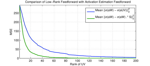
Figure 2 illustrates the error profile of a neural network using the low-rank estimation $UV$ in place of $W$ compared with a neural network augmented with an activation sign estimator as the rank is varied from one to full-rank. One can see that the error of the activation sign estimator diminishes far more quickly than the error of the low-rank activation, implying that the sign estimator can do well with a relatively low-rank approximation of $W$.

3.2 SVD as a Low-Rank Approximation

The Singular Value Decomposition (SVD) is a common matrix decomposition technique that factorizes a matrix $A\in\mathbb{R}^{m\times n}$ into $A=U\Sigma V^{T}$, $U\in\mathbb{R}^{m\times m},\Sigma\in\mathbb{R}^{m\times n},V\in\mathbb{R}^{n\times n}$. By [6], the matrix $A$ can be approximated using a low rank matrix $\hat{A}_{r}$ corresponding to the solution of the constrained optimization of

$$\min_{\hat{A}_{r}}\|A-\hat{A}_{r}\|_{F}$$ (6)

where $\|\cdot\|_{F}$ is the Frobenius norm, and $\hat{A}_{r}$ is constrained to be of rank $r<rank(A)$. The minimizer $\hat{A}_{r}$ is given by taking the first $r$ columns of $U$, the first $r$ diagonal entries of $\Sigma$, and the first $r$ columns of $V$. The resulting matrices $U_{r}$, $\Sigma_{r}$, and $V_{r}$ are multiplied, yielding $\hat{A}_{r}=U_{r}\Sigma_{r}V_{r}^{T}$. The low-rank approximation $\hat{W}=UV$ is then defined such that $\hat{W}=U_{r}(\Sigma_{r}V_{r}^{T})$, where $U=U_{r}$ and $V=\Sigma_{r}V_{r}^{T}$.

Unfortunately, calculating the SVD is an expensive operation, on the order of $O(mn^{2})$, so recalculating the SVD upon the completion of every minibatch adds significant overhead to the training procedure. Given that we are uniquely interested in estimating in the sign of $a_{l+1}=a_{l}W_{l}$, we can opt to calculate the SVD less frequently than once per minibatch, assuming that the weights $W_{l}$ do not change significantly over the course of a single epoch so as to corrupt the sign estimation.

3.3 Encouraging Neural Network Sparsity

To overcome the additional overhead imposed by the conditional computation architecture, the neural network must have sparse activations. Without encouragement to settle on weights that result in sparse activations, such as penalties on the loss function, a neural network will not necessarily become sparse enough to be useful in the context of conditional computation. Therefore, an $\ell_{1}$ penalty for the activation vector of each layer is applied to the overall loss function, such that

$$J(W,\lambda)=L(W)+\lambda\sum_{l=1}^{L}\|a_{l}\|_{1}$$ (7)

Such a penalty is commonly used in sparse dictionary learning algorithms and tends to push elements of $a_{l}$ towards zero [13].

Dropout regularization [9] is another technique known to sparsify the hidden activations in a neural network. Dropout first sets the hidden activations $a_{l}$ to zero with probability $p$. During training, the number of active neurons is likely less than $p$ for each minibatch. When the regularized network is running in the inference mode, dropout has been observed to have a sparsifying effect on the hidden activations [17]. The adaptive dropout method [1] can further decrease the number of active neurons without degrading the performance of the network.

3.4 Theoretical Speed Gain

For every input example, a standard neural network computes $\sigma\left(aW\right)$, where $a\in\mathbb{R}^{N\times d}$ and $W\in\mathbb{R}^{d\times h}$, where $N=1$ for a fully-connected network, or $N$ is the number of convolutions for a convolutional network. Assuming additions and multiplications are constant-time operations, the matrix multiplication requires $N\left(2d-1\right)h$ floating point operations (we need to compute $Nh$ dot products, where each dot product consists of $d$ multiplications and $d-1$ additions), and the activation function requires $Nh$ floating point operations, yielding $N\left(2d-1\right)h+Nh$ operations. The activation estimator $\sigma\left(aUV\right)$, $U\in\mathbb{R}^{d\times k}$, $V\in\mathbb{R}^{k\times h}$ requires $N\left(2d-1\right)k+N\left(2k-1\right)h$ floating point operations for the low-rank multiplication followed by $Nh$ operations for the $sgn\left(\cdot\right)$ activation function, yielding $N\left(2d-1\right)k+N\left(2k-1\right)h+Nh$. However, given a sparsity coefficient $\alpha\in\left[0,1\right]$ (where $\alpha=0$ implies no activations are active, and $\alpha=1$ implies all activations are active), a conditional matrix multiplication would require $\alpha N\left(2d-1\right)h+\alpha Nh$ operations. The SVD calculation to obtain the activation estimation weights is $\beta O\left(nd\min\left(n,d\right)\right)$, where $\beta$ is the ratio of feed-forwards to SVD updates (eg., with a minibatch size of 250, a training set size of 50,000, and once-per-epoch SVD updates, $\beta=\frac{250}{50000}=0.005$).

Altogether, the number of floating point operations for calculating the feed-forward in a layer in a standard neural network is

$$F_{nn}=N\left(2d-1\right)h+Nh$$ (8)

and the number of floating point operations for the activation estimation network with conditional computation is

$$F_{ae}=N\left(2d-1\right)k+N\left(2k-1\right)h+Nh+\alpha h\left(N\left(2d-1\right)h+Nh\right)+\beta O\left(nd\min\left(n,d\right)\right)$$ (9)

The relative reduction of floating point operations for a layer can be represented as $\frac{F_{nn}}{F_{ae}}$, and is simplified as

$$\frac{2dh}{k\left(2d+2h-1\right)+2\alpha dh+\beta O\left(nd\min\left(n,d\right)\right)}$$ (10)

For a neural network with many layers, the relative speedup is given by

$$\frac{{\displaystyle\sum_{i=1}^{L}F_{nn}^{\left(l\right)}}}{{\displaystyle\sum_{i=1}^{L}F_{ae}^{\left(l\right)}}}$$ (11)

where ${\displaystyle F_{nn}^{\left(l\right)}}$ is the number of floating point operations for the $l^{th}$ layer of the full network, and ${\displaystyle F_{ae}^{\left(l\right)}}$ is the number of floating point operations for the $l^{th}$ layer of the network augmented by the activation estimation network. The overall speedup is greatly dependent on the sparsity of the network and the overhead of the activation estimator.

3.5 Implementation Details

The neural network is built using Rasmus Berg Palm’s Deep Learning Toolbox [16]. All hidden units are rectified-linear, and the output units are softmax trained with a negative log-likelihood loss function. The weights, $w$, are initialized as $w\sim\mathcal{N}\left(0,\sigma^{2}\right)$ and biases $b$ are set to 1 in order to encourage the neurons to operate in their non-saturated region once training begins, as suggested in [11]. In all experiments, the dropout probability $p$ is fixed to 0.5 for the hidden layers.

The learning rate $\gamma$ is scheduled such that $\gamma_{n}=\gamma_{0}\lambda^{n}$ where $\gamma_{n}$ is the learning rate for the $n^{th}$ epoch, $\gamma_{0}$ is the initial learning rate, and $\lambda$ is a decay term slightly less than 1, eg., 0.995. The momentum term $\nu$ is scheduled such that $\nu_{n}=\max\left(\nu_{max},\nu_{0}\beta^{n}\right)$ where $\nu_{n}$ is the momentum for the $n^{th}$ epoch, $\nu_{max}$ is the maximum allowed momentum, $\nu_{0}$ is the initial momentum, and $\beta$ is an incremental term slightly greater than 1, eg., 1.05.

To simplify prototyping, the feed-forward is calculated for a layer, and the activation estimator is immediately applied before the next layer activations are used. This is equivalent to bypassing the calculations for activations that are likely to produce zeros. In practice, re-calculating the SVD once per epoch for the activation estimator seems to be a decent tradeoff between activation estimation accuracy and computational efficiency, but this may not necessarily be true for other datasets.

4 Experimental Results

4.1 SVHN

	SVHN	MNIST
Architecture	1024-1500-700-400-200-10	784-1000-600-400-10
Weight Init	$w\sim\mathcal{N}\left(0,0.01\right)$; $b=1$	$w\sim\mathcal{N}\left(0,0.05\right)$; $b=1$
Init Learning Rate	0.15	0.25
Learning Rate Scaling	0.99	0.99
Maximum Momentum	0.8	0.8
Momentum Increment	1.01	1.05
Maximum Norm	25	25
$\ell_{1}$ Activation Penalty	0	$1\times 10^{-5}$
$\ell_{2}$Weight Penalty	–	$5\times 10^{-5}$

Table 1: Hyperparameters for SVHN and MNIST experiments.

Figure 3: Classification error of the validation set for SVHN on seven configurations of the activation estimator for each hidden layer. The ’control’ network has no activation estimator and is used as a baseline of comparison for the other networks.

Street View House Numbers (SVHN) [15] is a large image dataset containing over 600,000 labeled examples of digits taken from street signs. Each example is an RGB $32\times 32$ (3072-dimensional) image. To pre-process the dataset, each image is transformed into the YUV colorspace. Next, local contrast normalization [10] followed by a histogram equalization is applied to the Y channel. The U and V channels are discarded, resulting in a 1024-dimensional vector per example. The dataset is then normalized for the neural network by subtracting out the mean and dividing by the square root of the variance for each variable. To select the hyperparameters, the training data was split into 590,000 samples for the training set and 14,388 samples for the validation set. The architecture was held fixed while the other hyperparameters were chosen randomly over 30 runs using a network with no activation estimation. The hyperparameters of the neural network with the lowest resulting validation error were then used for all experiments.

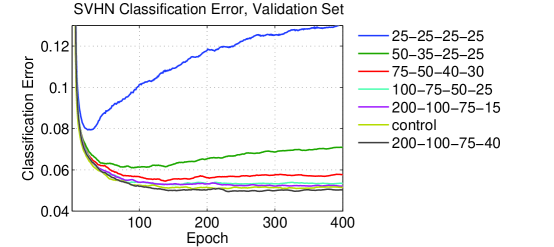
To evaluate the sensitivity of the activation estimator, several parameterizations for the activation estimator are evaluated. Each network is trained with the hyperparameters in Table 1, and the results of seven parameterizations are shown in Figure 3. Each parameterization is described by the rank of each approximation, eg., ‘75-50-40-30’ describes a network with an activation estimator using a 75-rank approximation for $W_{1}$, a 50-rank approximation for $W_{2}$, a 40-rank approximation for $W_{3}$, and a 30-rank approximation for $W_{4}$. Note that a low-rank approximation is not necessary for $W_{5}$ (the weights connecting the last hidden layer to the output layer), as we do not want to approximate the activations for the output layer.

Figure 4: A comparison of a low-rank activation estimator and a higher-rank activation estimator. In this instance, a 25-25-25-25 activation estimator is too coarse to adequately capture the structure of the weight matrices.

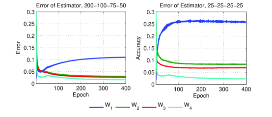
Some runs, specifically 25-25-25-25 and 50-35-25-25 in Figure 3 exhibit an initial decrease in classification error, followed by a gradual increase in classification error as training progresses. In the initial epochs, the hidden layer activations are mostly positive because the weights are relatively small and the biases are very large. As a consequence, the activation estimation is a much simpler task for the initial epochs. However, as the pattern of the activation signs diversifies as the network continues to train, the lower-rank approximations begin to fail, as illustrated in Figure 4.

Table 2 summarizes the test set error for the control and activation estimation networks. $W_{1}$ appears to be most sensitive, quickly reducing the test set error from 10.72% to 12.16% when the rank of $\hat{W}_{1}$ is lowered from 75 to 50. The rank of $\hat{W}_{4}$ appears to be the least sensitive, reducing the test set error from 9.96% to 10.01% as the rank is lowered from 25 to 15.

Network	Error
Control	9.31%
200-100-75-15	9.67%
100-75-50-25	9.96%
100-75-50-15	10.01%
75-50-40-30	10.72%
50-40-40-35	12.16%
25-25-15-15	19.40%

Table 2: SVHN test set error for seven networks.

4.2 MNIST

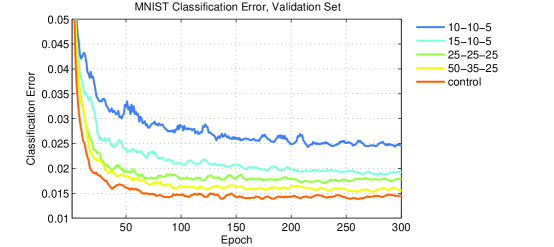
MNIST is a well-known dataset of hand-written digits containing 70,000 $28\times 28$ labeled images, and is generally split into 60,000 training and 10,000 testing examples. Very little pre-processing is required to achieve good results - each feature is transformed by $x_{t}=\frac{x}{\sqrt{\sigma_{max}^{2}}}-0.5$, where $x$ is the input feature, $\sigma_{max}^{2}$ is the maximum variance of all features, and 0.5 is a constant term to roughly center each feature. To select the hyperparameters, the training data was split into 50,000 samples for the training set and 10,000 samples for the validation set. The architecture was held fixed while the other hyperparameters were chosen randomly over 30 runs using a network with no activation estimation. The hyperparameters of the neural network with the lowest resulting validation error were then used for all experiments. Several parameterizations for the activation estimator are evaluated for a neural network trained with the hyperparameters listed in Table 1 using the same approach as the SVHN experiment above. The results for the validation set plotted against the epoch number are shown in Figure 5, and the final test set accuracy is reported in Table 3.

A neural network with a very low-rank weight matrix in the activation estimation can train surprisingly well on MNIST. Lowering the rank from 784-600-400 to 50-35-25 impacts performance negligibly. Ranks as low as 25-25-25 does not lessen performance too greatly, and ranks as low as 10-10-5 yield a classifier capable of 2.28% error.

Figure 5: Classification error of the validation set for MNIST on five configurations of the activation estimator for each hidden layer.

Network	Error
Control	1.40%
50-35-25	1.43%
25-25-25	1.60%
15-10-5	1.85%
10-10-5	2.28%

Table 3: MNIST test set error for five networks.

5 Discussion and Further Work

Low-rank estimations of weight matrices of a neural network obtained via once-per-epoch SVD work very well as efficient estimators of the sign of the activation for the next hidden layer. In the context of rectified-linear hidden units, computation time can be reduced greatly if this estimation is reliable and the hidden activations are sufficiently sparse. This approach is applicable to any hard-thresholding activation function, such as the functions investigated in [8], and can be easily extended to be used with convolutional neural networks.

Figure 6: Because the SVD is calculated at the beginning of each epoch, each subsequent gradient update in each minibatch moves the weight matrix further from low-rank factorization, resulting in an increasing error until the SVD is recalculated at the beginning of the next epoch. Different layers are negatively impacted in differing degrees.

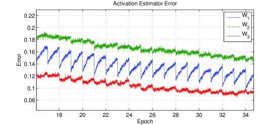
While the activation estimation error does not tend to deviate too greatly inbetween minibatches over an epoch, as illustrated in Figure 6, this is not guaranteed. An online approach to the low-rank approximation would therefore be preferable to a once-per-epoch calculation. In addition, while the low-rank approximation given by SVD minimizes the objective function $\|A-\hat{A}_{r}\|_{F}$, this is not necessarily the best objective function for an activation estimator, where we seek to minimize $\left\|\sigma\left(aW\right)-\sigma\left(aW\cdot S\right)\right\|$, which is a much more difficult and non-convex objective function. Also, setting the hyperparameters for the activation estimator can be a tedious process involving expensive cross-validation when an adaptive algorithm could instead choose the rank based on the spectrum of the singular values. Therefore, developing a more suitable low-rank approximation algorithm could provide a promising future direction of research.

In [1], the authors propose a method called “adaptive dropout” by which the dropout probabilities are chosen by a function optimized by gradient descent instead of fixed to some value. This approach bears some resemblance to this paper, but with the key difference that the approach in [1] is motivated by improved regularization and this paper’s method is motivated by computational efficiency. However, the authors introduce a biasing term that allows for greater sparsity that could be introduced into this paper’s methodology. By modifying the conditional computation unit to compute $sgn\left(aUV-b\right)$, where $b$ is some bias, we can introduce a parameter that can tune the sparsity of the network, allowing for a more powerful trade-off between accuracy and computational efficiency.

Acknowledgments

This work was partially supported by the Defense Advanced Research Projects Agency (DARPA) under contract number HR0011-13-2-0016.

References

- [1] Jimmy Ba and Brendan Frey. Adaptive dropout for training deep neural networks. In Advances in Neural Information Processing Systems, pages 3084–3092, 2013.
- [2] Yoshua Bengio. Deep learning of representations: Looking forward. In Adrian-Horia Dediu, Carlos Martin-Vide, Ruslan Mitkov, and Bianca Truthe, editors, Statistical Language and Speech Processing, volume 7978 of Lecture Notes in Computer Science, pages 1–37. Springer Berlin Heidelberg, 2013.
- [3] Yoshua Bengio, Nicholas Léonard, and Aaron C. Courville. Estimating or propagating gradients through stochastic neurons for conditional computation. CoRR, abs/1308.3432, 2013.
- [4] Adam Coates, Brody Huval, Tao Wang, David Wu, Bryan Catanzaro, and Ng Andrew. Deep learning with cots hpc systems. In Proceedings of the 30th International Conference on Machine Learning (ICML-13), pages 1337–1345, 2013.
- [5] Misha Denil, Babak Shakibi, Laurent Dinh, Marc’Aurelio Ranzato, and Nando de Freitas. Predicting parameters in deep learning. arXiv preprint arXiv:1306.0543, 2013.
- [6] Carl Eckart and Gale Young. The approximation of one matrix by another of lower rank. Psychometrika, 1(3):211–218, 1936.
- [7] Xavier Glorot, Antoine Bordes, and Yoshua Bengio. Deep sparse rectifier networks. In Proceedings of the 14th International Conference on Artificial Intelligence and Statistics. JMLR W&CP Volume, volume 15, pages 315–323, 2011.
- [8] Rostislav Goroshin and Yann LeCun. Saturating auto-encoder. arXiv preprint arXiv:1301.3577, 2013.
- [9] Geoffrey E Hinton, Nitish Srivastava, Alex Krizhevsky, Ilya Sutskever, and Ruslan R Salakhutdinov. Improving neural networks by preventing co-adaptation of feature detectors. arXiv preprint arXiv:1207.0580, 2012.
- [10] Kevin Jarrett, Koray Kavukcuoglu, Marc’Aurelio Ranzato, and Yann LeCun. What is the best multi-stage architecture for object recognition? In Computer Vision, 2009 IEEE 12th International Conference on, pages 2146–2153. IEEE, 2009.
- [11] Alex Krizhevsky, Ilya Sutskever, and Geoff Hinton. Imagenet classification with deep convolutional neural networks. In Advances in Neural Information Processing Systems 25, pages 1106–1114, 2012.
- [12] Quoc Le, Marc’Aurelio Ranzato, Rajat Monga, Matthieu Devin, Kai Chen, Greg Corrado, Jeff Dean, and Andrew Ng. Building high-level features using large scale unsupervised learning. In International Conference in Machine Learning, 2012.
- [13] Honglak Lee, Alexis Battle, Rajat Raina, and Andrew Ng. Efficient sparse coding algorithms. In Advances in neural information processing systems, pages 801–808, 2006.
- [14] A Mohamed, Tara N Sainath, George Dahl, Bhuvana Ramabhadran, Geoffrey E Hinton, and Michael A Picheny. Deep belief networks using discriminative features for phone recognition. In Acoustics, Speech and Signal Processing (ICASSP), 2011 IEEE International Conference on, pages 5060–5063. IEEE, 2011.
- [15] Yuval Netzer, Tao Wang, Adam Coates, Alessandro Bissacco, Bo Wu, and Andrew Y Ng. Reading digits in natural images with unsupervised feature learning.
- [16] R. B. Palm. Prediction as a candidate for learning deep hierarchical models of data, 2012.
- [17] Nitish Srivastava. Improving neural networks with dropout. PhD thesis, University of Toronto, 2013.