Single-trial estimation of stimulus and spike-history effects on time-varying ensemble spiking activity of multiple neurons: a simulation study

Abstract

Neurons in cortical circuits exhibit coordinated spiking activity, and can produce correlated synchronous spikes during behavior and cognition. We recently developed a method for estimating the dynamics of correlated ensemble activity by combining a model of simultaneous neuronal interactions (e.g., a spin-glass model) with a state-space method (Shimazaki et al. 2012 PLoS Comput Biol 8 e1002385). This method allows us to estimate stimulus-evoked dynamics of neuronal interactions which is reproducible in repeated trials under identical experimental conditions. However, the method may not be suitable for detecting stimulus responses if the neuronal dynamics exhibits significant variability across trials. In addition, the previous model does not include effects of past spiking activity of the neurons on the current state of ensemble activity. In this study, we develop a parametric method for simultaneously estimating the stimulus and spike-history effects on the ensemble activity from single-trial data even if the neurons exhibit dynamics that is largely unrelated to these effects. For this goal, we model ensemble neuronal activity as a latent process and include the stimulus and spike-history effects as exogenous inputs to the latent process. We develop an expectation-maximization algorithm that simultaneously achieves estimation of the latent process, stimulus responses, and spike-history effects. The proposed method is useful to analyze an interaction of internal cortical states and sensory evoked activity.

1 Introduction

Neurons in the brain make synaptic contacts to each other and form specific signaling networks. A typical cortical neuron receives synaptic inputs from $3000-10000$ other neurons, and makes synaptic contacts to several thousands of other neurons. They send and receive signals using pulsed electrical discharges known as action potentials, or spikes. Therefore, individual neurons in a circuit can be activated in a coordinated manner when relevant information is processed. In particular, nearly simultaneous spiking activity of multiple neurons (synchronous spikes) occurs dynamically in relation to a stimulus presented to an animal, the animal’s behavior, and the internal state of the brain (attention and expectation) [1, 2, 3, 4, 5].

Recently, it was reported that a model of synchronous spiking activity that accounts for spike rates of individual neurons and interactions between pairs of neurons can explain $\sim 90$% of the synchronous spiking activity of a small subset ($\sim 10$) of retinal ganglion cells [6, 7] and cortical neurons [8] in vitro. This model is known as a maximum entropy model or an Ising/spin-glass model in statistical physics. However, since the model assumes stationary data, it is not directly applicable to non-stationary data recorded from awake behaving animals. In these data sets, spike-rates of individual neurons and even interactions among them may vary across time.

In order to analyze time-dependent synchronous activity of neurons, we recently developed a method for estimating the dynamics of correlations between neurons by combining the model of neuronal interactions (e.g., the Ising/spin-glass model) with a state-space method [9, 10]. In classical neurophysiological experiments, neuronal activity is repeatedly recorded under identical experimental conditions in order to obtain reproducible features in the spiking activity across the ‘trials’. Typically, neurophysiologists estimate average time-varying firing rates of individual neurons in response to a stimulus from the repeated trials [11, 12]. In the same fashion, the state-space method in [9, 10] aims to estimate the dynamics of the neuronal interactions, including higher-order interactions, that occurs repeatedly upon the onset of externally triggered events. When this method is applied to three neurons recorded simultaneously from the primary motor cortex of a monkey engaged in a delayed motor task (data from [2]), it was revealed that these neurons dynamically organized into a group characterized by the presence of a higher-order (triple-wise) interaction, depending on the behavioral demands to the monkey [12].

However, neurophysiological studies in the past decades revealed that spiking activity of individual neurons is subject to large variability across trials due to structured ongoing activity of the networks that arises internally to the brain [13, 14, 15]. In these conditions, the method developed in [12] would not efficiently detect the stimulus responses because a signal-to-noise ratio may be small even in the trial-averaged activity. Although statistical methods for detecting responses of individual neurons from single-trial data have been investigated [16, 17, 18, 19], no methods are available for estimating synchronous responses of multiple neurons to a stimulus in a single trial when these neurons are subject to the activity that is largely unrelated to the stimulus.

In the analysis of single-trial data, it is critical to consider dependency of the current activity of neurons on the past history of their activity. A neuron undergoes an inactivation period known as a refractory period after it generates an action potential. Therefore, a model neuron significantly improves its goodness-of-fit to data if it captures this biophysical property [20, 21]. In addition, estimating the dependency of the current activity level of a neuron on past spiking history of another neuron allows us to construct effective connectivity of the network within an observed set of neurons [22, 23]. Including the spike-history effects in the models of synchronous ensemble activity is thus an important topic, and investigated also in [24] in the framework of a continuous-time point process theory.

In this study we construct a method for simultaneously estimating the stimulus and spike-history effects on ensemble spiking activity when the activity of these neurons is dominated by ongoing activity. For this goal, we extend the previously developed state-space model of neuronal interactions: We model the ongoing activity, i.e., time-varying spike rates and interactions, of neurons as a latent process, and include the stimulus and spike-history effects on the activity as exogenous inputs to the latent process. We develop an expectation-maximization (EM) algorithm for this model, which efficiently combines construction of a posterior density of the latent process and estimation of the parameters for stimulus and spike-history effects. The method is tested using simulated spiking activity of 3 neurons with known underlying architecture. We provide an approximation method for determining inclusion of these exogenous inputs in the model and a surrogate method to test significance of the estimated parameters.

2 Methods

In this study, we analyze spike sequences simultaneously obtained from $N$ neurons. From these spike sequences, we construct binary spike patterns at discrete time steps by dividing the sequences into disjoint time bins with an equal width of $\Delta$ ms (in total, $T$ bins). The width $\Delta$ determines a permissible range of synchronous activity of neurons in this analysis. We let $X_{i}^{t}$ be a binary variable of the $i$-th neuron ($i=1,2,\ldots,N$) in the $t$-th time bin ($t=1,2,\ldots,T$). Here a time bin containing ‘$1$’ indicates that one or more spikes exist in the time bin whereas ‘$0$’ indicates that no spike exists in the time bin. The binary pattern of $N$ neurons at time bin $t$ is denoted as $\mathbf{X}_{t}=[X_{1}^{t},X_{2}^{t},\ldots,X_{N}^{t}]^{\prime}$. The prime indicates the transposition operation to the vector. The entire observation of the discretized ensemble spiking activity is represented as $\mathbf{X}_{1:T}=[\mathbf{X}_{1},\mathbf{X}_{2},\ldots,\mathbf{X}_{T}]$.

2.1 The model of time-varying simultaneous interactions of neurons

We analyze the ensemble spike patterns using time-dependent formulation of a joint probability mass function for binary random variables. Let $x_{i}$ be a binary variable, namely $x_{i}=\left\{0,1\right\}$. The joint probability mass function of $N$-tuple binary variables, $\mathbf{x}=[x_{1},x_{2},\ldots,x_{N}]$, at time bin $t$ ($t=1,2,\ldots,T$) can be written in an exponential form as

$$p(\mathbf{x}|\boldsymbol{\theta}_{t}) =\exp\left[\sum_{i}\theta_{i}^{t}x_{i}+\sum_{i<j}\theta_{ij}^{t}x_{i}x_{j}+\cdots+\theta_{1\cdots N}^{t}x_{1}\cdots x_{N}-\psi(\boldsymbol{\theta}_{t})\right].$$ (1)

Here $\boldsymbol{\theta}_{t}=[\theta_{1}^{t},\theta_{2}^{t},\ldots,\theta_{12}^{t},\theta_{13}^{t},\ldots,\theta_{1\cdots N}^{t}]^{\prime}$ summarizes the time-dependent canonical parameters of the exponential family distribution. The canonical parameters for the interaction terms, e.g., $\theta_{ij}^{t}$ ($i,j=1,\ldots,N$), represent time-dependent instantaneous interactions at time bin $t$ among the neurons denoted in its subscript. $\psi(\boldsymbol{\theta}_{t})$ is a log normalization parameter to satisfy $\sum p(\mathbf{x}|\boldsymbol{\theta}_{t})=1$.

Using a feature vector that captures simultaneous spiking activities of subsets of the neurons, $\mathbf{f}=[f_{1},f_{2},\ldots,f_{12},f_{13},\ldots,f_{1\cdots N}]^{\prime}$, where

$$\begin{array}[]{cc}f_{i}\left(\mathbf{x}\right)=x_{i},&i=1,\cdots,N\\ f_{ij}\left(\mathbf{x}\right)=x_{i}x_{j},&i<j\\ \vdots&\mbox{}\\ f_{1\cdots N}\left(\mathbf{x}\right)=x_{1}\cdots x_{N},&\mbox{}\end{array}$$

the probability mass function (Eq. 1) is compactly written as $p({\mathbf{x}}|\boldsymbol{\theta}_{t})=\exp\left[\boldsymbol{\theta}_{t}^{\prime}\mathbf{f}\left(\mathbf{x}\right)-\psi(\boldsymbol{\theta}_{t})\right]$. The expected occurrence rates of simultaneous spikes of multiple neurons is given by a vector $\boldsymbol{\eta}_{t}=E\left[\mathbf{f}\left(\mathbf{x}\right)|\boldsymbol{\theta}_{t}\right]$, where expectation is performed using $p({\mathbf{x}}|\boldsymbol{\theta}_{t})$.

Eq. 1 specifies the probabilities of all $2^{N}$ spike patterns by using $2^{N}-1$ parameters. One reasonable approach to reduce the number of parameters is to select and fix interesting features in the spiking activity, and construct a probability model that maximizes entropy. For example, maximization of entropy of the spike patterns given the low-order features, $\mathbf{f}=[f_{1},f_{2},\ldots,f_{N},f_{12},f_{13},\ldots,f_{N-1,N}]^{\prime}$, yields a spin-glass model that is similar to Eq. 1, but does not include interactions higher than the second order. While it is important to explore a characteristic feature vector to neuronal ensembles, here we note that the method developed in this study does not depend on the choice of the vector, $\mathbf{f}$. Below, we denote $d$ as the number of elements in the vector, $\mathbf{f}$.

Given the observed ensemble spiking activity $\mathbf{X}_{1:T}$, the likelihood function of $\boldsymbol{\theta}_{1:T}=[\boldsymbol{\theta}_{1},\boldsymbol{\theta}_{2},\ldots,\boldsymbol{\theta}_{T}]$ is given as

$$p\left(\mathbf{X}_{1:T}|\boldsymbol{\theta}_{1:T}\right) =\prod\limits_{t=1}^{T}\exp[\boldsymbol{\theta}_{t}^{\prime}\mathbf{f}\left(\mathbf{X}_{t}\right)-\psi(\boldsymbol{\theta}_{t})],$$ (2)

assuming conditional independence across the time bins. Eq.2 constitutes an observation equation of our state-space model.

2.2 Inclusion of stimulus and spike-history effects in the state model

The main focus of attention in this study is modeling of a process for the time-dependent canonical parameters, $\boldsymbol{\theta}_{t}$, in Eq. 1. We model their evolution as a first-order auto-regressive (AR) model. The effects of the stimulus and spike history are included as exogenous inputs to the AR model (an ARX model). In its full expression, the state model is written as

$$\boldsymbol{\theta}_{t}=\mathbf{F}\boldsymbol{\theta}_{t-1}+\mathbf{G}\mathbf{S}_{t}+\sum_{i=1}^{p}\mathbf{H}_{i}\mathbf{X}_{t-i}+\boldsymbol{\xi}_{t},$$ (3)

for $t=2,\ldots,T$. Here the matrix $\mathbf{F}$ ($d\times d$ matrix) is the first order auto-regressive parameter. $\boldsymbol{\xi}_{t}$ ($d\times 1$ matrix) is a random vector independently drawn from a zero-mean multivariate normal distribution with covariance matrix $\mathbf{Q}$ ($d\times d$ matrix) at each time bin. The state process starts with an initial value $\boldsymbol{\theta}_{1}$ that follows a normal distribution with mean $\boldsymbol{\mu}$ ($d\times 1$ matrix) and covariance matrix $\boldsymbol{\Sigma}$ ($d\times d$ matrix), namely $\boldsymbol{\theta}_{1}\sim\mathcal{N}\left(\boldsymbol{\mu},\boldsymbol{\Sigma}\right)$. Below, we describe details of the exogenous terms.

The second term represents responses to external signals, or stimuli, $\mathbf{S}_{t}$, which are observed concurrently with the spike sequences. The vector $\mathbf{S}_{t}$ is a column vector of $n_{s}$ external signals at time bin $t$. The each element is the value of an external signal at time bin $t$. If an external signal is represented as a sequence of discrete events, we denote the corresponding element of $\mathbf{S}_{t}$ by ‘1’ if an event occurred within time bin $t$ and ‘0’ otherwise. Multiplying $\mathbf{S}_{t}$ by the matrix $\mathbf{G}$ ($d\times n_{s}$ matrix) produces weighted linear combinations of the external signals at time bin $t$.

The third term represents the effects of spiking activity during the previous $p$ time bins, $\mathbf{X}_{t-i}$ $(i=1,\ldots,p)$, on the current activity. The matrix $\mathbf{H}_{i}$ ($d\times N$ matrix) represents the spike-history effects of spiking activity in the previous time bin $t-i$ on the state at time bin $t$. The spike-history effects are collectively denoted as $\mathbf{H}\equiv[\mathbf{H}_{1},\mathbf{H}_{2},\ldots,\mathbf{H}_{p}]$ ($d\times Np$ matrix).

Eq. 3 constitutes a prior density of the latent process in our state-space model. We denote the set of parameters in the prior distribution, called hyper-parameters, as $\mathbf{w}\equiv\left[\mathbf{F},\mathbf{G},\mathbf{H},\mathbf{Q},\boldsymbol{\mu},\boldsymbol{\Sigma}\right]$. In this study, we refer to $\mathbf{w}$ as a parameter. In addition, we simplify Eq. 3 as $\boldsymbol{\theta}_{t}=\mathbf{F}\boldsymbol{\theta}_{t-1}+\mathbf{U}\mathbf{u}_{t}+\boldsymbol{\xi}_{t},$ where $\mathbf{u}_{t}$ is a single column vector constructed by stacking the stimulus vector and spike-history vectors at time bin $t$ in a row, i.e., $\mathbf{u}_{t}=[\mathbf{S}_{t};\mathbf{X}_{t-1};\mathbf{X}_{t-2};\ldots;\mathbf{X}_{t-p}]$. Similarly, we define a matrix $\mathbf{U}$ as $\mathbf{U}=[\mathbf{G},\mathbf{H}]$. With this simplification, the prior density defined in Eq. 3 is written as $p(\boldsymbol{\theta}_{1:T}|\mathbf{w})=p(\boldsymbol{\theta}_{1}|\boldsymbol{\mu},\boldsymbol{\Sigma})\prod_{t=2}^{T}p(\boldsymbol{\theta}_{t}|\boldsymbol{\theta}_{t-1},\mathbf{F},\mathbf{U},\mathbf{Q})$, where the transition probability, $p(\boldsymbol{\theta}_{t}|\boldsymbol{\theta}_{t-1},\mathbf{F},\mathbf{U},\mathbf{Q})$, is given as a normal distribution with mean $\mathbf{F}\boldsymbol{\theta}_{t-1}+\mathbf{U}\mathbf{u}_{t}$ and covariance matrix $\mathbf{Q}$.

3 Estimation of stimulus responses and spike-history effects

We estimate the parameter, $\mathbf{w}$, based on the principle of maximizing a (log) marginal likelihood function. Namely, we select the parameter that maximizes

$$l\left(\mathbf{w}\right)=\log\int p\left(\mathbf{X}_{1:T},\boldsymbol{\theta}_{1:T}|\mathbf{w}\right)d\boldsymbol{\theta}_{1:T}.$$ (4)

For this goal, we use the expectation-maximization (EM) algorithm [25, 26, 27]. In this method, we iteratively obtain the optimal parameter $\mathbf{\mathbf{w}^{\ast}}$ that maximizes the lower bound of the above log marginal likelihood. This alternative function, known as the expected complete data log-likelihood (a.k.a., $q$-function), is computed as

$$q\left(\mathbf{\mathbf{w}^{\ast}}|\mathbf{w}\right) \equiv E\left[\log p\left(\mathbf{X}_{1:T},\boldsymbol{\mathbf{\theta}}_{1:T}|\mathbf{\mathbf{w}^{\ast}}\right)|\mathbf{X}_{1:T},\mathbf{w}\right]$$

$$=\sum\limits_{t=1}^{T}\left(E\boldsymbol{\theta}^{\prime}_{t}\mathbf{f}\left(\mathbf{X}_{t}\right)-E\psi\left(\boldsymbol{\theta}_{t}\right)\right)-\frac{d}{2}\log{2\pi}-\frac{1}{2}\log{\det\boldsymbol{\Sigma}^{\ast}}$$

$$-\frac{1}{2}E[\left(\boldsymbol{\theta}_{1}-\boldsymbol{\mu}^{\ast}\right)^{\prime}\boldsymbol{\Sigma}^{\ast-1}\left(\boldsymbol{\theta}_{1}-\boldsymbol{\mu}^{\ast}\right)]-\frac{\left(T-1\right)d}{2}\log{2\pi}-\frac{\left(T-1\right)}{2}\log{\det\mathbf{Q}^{\ast}}$$

$$-\frac{1}{2}\sum\limits_{t=2}^{T}E[\left(\boldsymbol{\theta}_{t}-\mathbf{F}^{\ast}\boldsymbol{\theta}_{t-1}-\mathbf{U}^{\ast}\mathbf{u}_{t}\right)^{\prime}\mathbf{Q}^{\ast-1}\left(\boldsymbol{\theta}_{t}-\mathbf{F}^{\ast}\boldsymbol{\theta}_{t-1}-\mathbf{U}^{\ast}\mathbf{u}_{t}\right)].$$ (5)

The expectation, $E[\centerdot|\mathbf{X}_{1:T},\mathbf{w}]$, in Eq. 5 is performed using the smoother posterior density of the state obtained by a nominal parameter, $\mathbf{w}$, namely

$$p\left(\boldsymbol{\theta}_{1:T}|\mathbf{X}_{1:T},\mathbf{w}\right)=\frac{p\left(\mathbf{X}_{1:T}|\boldsymbol{\theta}_{1:T}\right)p\left(\boldsymbol{\theta}_{1:T}|\mathbf{w}\right)}{p\left(\mathbf{X}_{1:T}|\mathbf{w}\right)}.$$ (6)

In particular, Eq. 5 can be computed using the following expected values by the posterior density: The smoother mean $\boldsymbol{\theta}_{t|T}=E\left[\boldsymbol{\theta}_{t}|\mathbf{X}_{1:T},\mathbf{w}\right]$, the smoother covariance matrix $W_{t|T}=E[(\boldsymbol{\theta}_{t}-\boldsymbol{\theta}_{t|T})(\boldsymbol{\theta}_{t}-\boldsymbol{\theta}_{t|T})^{\prime}|\mathbf{X}_{1:T},\mathbf{w}]$, and the lag-one covariance matrix, $W_{t,t-1|T}=E[(\boldsymbol{\theta}_{t}-\boldsymbol{\theta}_{t|T})(\boldsymbol{\theta}_{t-1}-\boldsymbol{\theta}_{t-1|T})^{\prime}|\mathbf{X}_{1:T},\mathbf{w}]$. These values are obtained using the approximate recursive Bayesian filtering/smoothing algorithm developed in [9, 10] (See Appendix A and Eqs. 22, 23, and 24 therein).

In the EM-algorithm, we obtain the parameter that maximizes the $q$-function by alternating the expectation (E) and maximization (M) steps. In the E-step, we obtain the above expected values in Eq. 5 by the approximate recursive Bayesian filtering/smoothing algorithm using a fixed $\mathbf{w}$ (Appendix A). In the M-step, we obtain the parameter, $\mathbf{\mathbf{w}^{\ast}}$, that maximizes Eq. 5. The resulting $\mathbf{\mathbf{w}^{\ast}}$ is then used in the next E-step. Below, we derive an algorithm for optimizing the parameter at the M-step.

For the state model that includes the auto-regressive parameter and stimulus and/or spike-history effects, these parameters are estimated simultaneously. From $\frac{\partial}{\partial\mathbf{F}^{\ast}}q\left(\mathbf{w}^{\ast}|\mathbf{w}\right)=\mathbf{0}$, we obtain

$$\mathbf{F}^{\ast}\sum_{t=2}^{T}\left(\mathbf{W}_{t-1,t|T}+\boldsymbol{\theta}_{t-1|T}\boldsymbol{\theta}_{t-1|T}^{\prime}\right)+\mathbf{U}^{\ast}\sum_{t=2}^{T}\boldsymbol{u}_{t}\boldsymbol{\theta}_{t-1|T}^{\prime}=\sum_{t=2}^{T}\left(\mathbf{W}_{t-1,t|T}+\boldsymbol{\theta}_{t|T}\boldsymbol{\theta}_{t-1|T}^{\prime}\right).$$ (7)

Here, $\boldsymbol{\theta}_{t|T}$, $\mathbf{W}_{t|T}$, and $\mathbf{W}_{t-1,t|T}$ are the smoother mean and covariance, and the lag-one covariance matrix given by Eqs. 22, 23, and 24, respectively. Similarly, from $\frac{\partial}{\partial\mathbf{U}^{\ast}}q\left(\mathbf{w}^{\ast}|\mathbf{w}\right)=\mathbf{0}$, we obtain

$$\mathbf{F}^{\ast}\sum_{t=2}^{T}\boldsymbol{\theta}_{t-1|T}\boldsymbol{u}_{t}^{\prime}+\mathbf{U}^{\ast}\sum_{t=2}^{T}\boldsymbol{u}_{t}\boldsymbol{u}_{t}^{\prime}=\sum_{t=2}^{T}\boldsymbol{\theta}_{t|T}\boldsymbol{u}_{t}^{\prime}.$$ (8)

Hence, the simultaneous update rule for $\mathbf{F}^{\ast}$ and $\mathbf{U}^{\ast}$ is given as

$$\left[\begin{array}[]{cc}\mathbf{F}^{\ast}&\mathbf{U}^{\ast}\end{array}\right] =\left[\begin{array}[]{cc}\sum_{t=2}^{T}\left(\mathbf{W}_{t-1,t|T}+\boldsymbol{\theta}_{t|T}\boldsymbol{\theta}_{t-1|T}^{\prime}\right)&\sum_{t=2}^{T}\boldsymbol{\theta}_{t|T}\boldsymbol{u}_{t}^{\prime}\end{array}\right]$$ (11)

$$\left[\begin{array}[]{cc}\sum_{t=2}^{T}\left(\mathbf{W}_{t-1,t|T}+\boldsymbol{\theta}_{t-1|T}\boldsymbol{\theta}_{t-1|T}^{\prime}\right)&\sum_{t=2}^{T}\boldsymbol{\theta}_{t-1|T}\boldsymbol{u}_{t}^{\prime}\\ \sum_{t=2}^{T}\boldsymbol{u}_{t}\boldsymbol{\theta}_{t-1|T}^{\prime}&\sum_{t=2}^{T}\boldsymbol{u}_{t}\boldsymbol{u}_{t}^{\prime}\end{array}\right]^{-1}.$$ (14)

Here the inverse matrix on the r.h.s. is obtained by using the blockwise inversion formula:

$$\left[\begin{array}[]{cc}A&B\\ C&D\end{array}\right]^{-1}=\left[\begin{array}[]{cc}A^{-1}+A^{-1}B\left(D-CA^{-1}B\right)^{-1}CA^{-1}&-A^{-1}B\left(D-CA^{-1}B\right)^{-1}\\ -\left(D-CA^{-1}B\right)^{-1}CA^{-1}&\left(D-CA^{-1}B\right)^{-1}\end{array}\right].$$

The covariance matrix, $\mathbf{Q}$, can be optimized separately. From $\frac{\partial}{\partial\mathbf{Q}^{\ast}}q\left(\mathbf{w}^{\ast}|\mathbf{w}\right)=\mathbf{0}$, the update rule of $\mathbf{Q}$ is obtained as

$$\mathbf{Q}^{\ast}= \frac{1}{T-1}\sum_{t=2}^{T}[\mathbf{W}_{t|T}-\mathbf{W}_{t-1,t|T}\mathbf{F}^{\prime}-\mathbf{FW}_{t-1,t|T}^{\prime}+\mathbf{FW}_{t-1|T}\mathbf{F}^{\prime}]$$

$$+ \frac{1}{T-1}\sum_{t=2}^{T}\left(\boldsymbol{\theta}_{t|T}-\mathbf{F}\boldsymbol{\theta}_{t-1|T}-\mathbf{U}\mathbf{u}_{t}\right)\left(\boldsymbol{\theta}_{t|T}-\mathbf{F}\boldsymbol{\theta}_{t-1|T}-\mathbf{U}\mathbf{u}_{t}\right)^{\prime}.$$ (15)

Finally, the mean of the initial distribution is updated with $\boldsymbol{\mu}^{\ast}=\boldsymbol{\theta}_{1|T}$ from $\frac{\partial}{\partial\boldsymbol{\mu}^{\ast}}q\left(\mathbf{w}^{\ast}|\mathbf{w}\right)=\mathbf{0}$. The covariance matrix $\boldsymbol{\Sigma}$ for the initial parameters is fixed in this optimization.

4 Results

4.1 Simulation of a network of 3 neurons

Figure 1: (A) Schematic diagram of a simulated network of 3 neurons. Neuron 1 makes excitatory synaptic contacts to Neuron 2 and 3. Stimulus 1 excites Neuron 1 whereas Stimulus 2 excites Neuron 2 and 3 simultaneously. In addition, all neurons receive sinusoidal rate modulation. (B) Simulated spiking activity of the network. A short period (1 s) of the total 30 s length is shown. The magenta and cyan triangles represent occurrence times of Stimulus 1 and 2, respectively. The gray bar highlights simultaneous spikes of Neuron 2 and 3 that are causally induced 5 ms after a spike occurs in Neuron 1. (C) Instantaneous spike rates. (Top) The red trace is the instantaneous spike rate of Neuron 1 simulated as an inhomogeneous renewal point process whos instantaneous inter-spike interval is given by the inverse Gaussian distribution ($f\left(t;\kappa\right)=\sqrt{\frac{\kappa}{2\pi t^{3}}}\exp\left[-\frac{\kappa}{2t}\left(t-1\right)^{2}\right]\text{for }x>0\text{, }0\text{ for }x<0$, $\kappa=1.8$ for all neurons). The inhomogeneous rate is modulated by the sinusoidal function (black solid line, frequency: 1 Hz; mean rate and amplitude: 30 spikes/s). (Bottom) Instantaneous spike rates of Neuron 2 and 3 (solid green line and dashed blue line, respectively).

In order to test the method, we simulate spiking activity of 3 neurons that possess specific characteristics in spike generation and connectivity as follows (See Fig. 1A). (1) The instantaneous firing rate of each neuron model depends on its own spike history in order to reproduce refractoriness in neuronal spiking activity. To achieve this, we adopt a renewal point process model whose instantaneous inter-spike interval (ISI) distribution is given by an inverse Gaussian distribution as a model of the stochastic spiking activity. (2) The firing rate of each neuron model varies across time in order to reproduce the ongoing activity. For that purpose, spike times of each neuron are generated from the renewal process by adding inhomogeneity to the underlying rate using the time-rescaling method described in [20]. The underlying rate of the inhomogeneous renewal point process model is modulated using a sinusoidal function (frequency: 1 Hz; mean and amplitude: 30 spikes/s). This rate modulation is common to the 3 neurons. (3) The neurons are activated by externally triggered stimulus inputs. To realize the stimulus responses, we deterministically induce spikes at predetermined timings of the stimuli. We consider two stimuli, one (Stimulus 1) that induces a spike in Neuron 1, and the other (Stimulus 2) that induces synchronous spikes in Neuron 2 and Neuron 3. The timings of external stimuli are not related to the sinusoidal time-varying rate, but randomly selected in the observation period (On average each stimulus happens once in 1 second). (4) There is feedforward circuitry in the network. We assume that Neuron 1 makes excitatory synaptic contacts to Neuron 2 and Neuron 3. To realize this, 5ms after a spike occurs in Neuron 1, we induce simultaneous spikes in Neuron 2 and Neuron 3 with a probability 0.5.

We simulate spike sequences with a length of 30 seconds using 1 ms resolution for numerical time steps (An example of a short period (1 s) is shown in Fig. 1B). Figure 1C displays the instantaneous spike-rates (conditional intensity functions of point processes) of Neuron 1 (Top, red line) and Neuron 2 & 3 (Bottom, green and blue lines) underlying the spiking activity in Fig. 1B. The black lines indicate sinusoidal rate modulation common to all neurons. In addition, spikes are induced in Neuron 1 at the onsets of Stimulus 1 (magenta triangles). Similarly, simultaneous spikes of Neuron 2 and Neuron 3 are generated at the onsets of Stimulus 2 (cyan triangles). In the traces of instantaneous spike-rates in Fig. 1C, instantaneous increases caused by the stimuli and synaptic inputs are not displayed. The instantaneous spike-rate of a neuron is reset to zero whenever a spike is induced in that neuron.

4.2 Selection of a state model

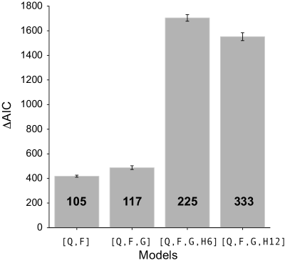
Figure 2: Comparison of state models by the Akaike Information Criterion (AIC). The state-space models with the following five different state models are comapared: [$\mathbb{Q}$], [$\mathbb{Q}$, $\mathbb{F}$],[$\mathbb{Q}$,$\mathbb{F}$,$\mathbb{G}$], [$\mathbb{Q}$,$\mathbb{F}$, $\mathbb{G}$, $\mathbb{H}6$], and [$\mathbb{Q}$,$\mathbb{F}$, $\mathbb{G}$, $\mathbb{H}12$] (See details of the models for main text). The reduction of the AIC of the last four models from the AIC of the model [$\mathbb{Q}$] ($\Delta$AIC) was repeatedly computed for 10 times. The height of the bar indicates the average $\Delta$AIC. The error bar indicates $\pm$ 2 S.E. The numbers marked on each bar are dimensions of the models (The number of free parameters in the state model).

We analyze the simulated ensemble activity by the proposed state-space model. For this goal, we first construct binary spike patterns, $\mathbf{X}_{1:T}$, from the simulated spike sequences of 30 seconds (Note: spike times are recorded in 1 ms resolution) by discretizing them using disjoint time bins with 2 ms width. We then apply state-space models to the binary data. The observation model used here contains interactions up to the second order (a pairwise interaction model):

$$p(\mathbf{x}|\boldsymbol{\theta}_{t}) =\exp\left[\theta_{1}^{t}x_{1}+\theta_{2}^{t}x_{2}+\theta_{3}^{t}x_{3}+\theta_{12}^{t}x_{1}x_{2}+\theta_{13}^{t}x_{1}x_{3}+\theta_{23}^{t}x_{2}x_{3}-\psi(\boldsymbol{\theta}_{t})\right].$$ (16)

For the state model, we consider 5 different models that include a set of different components in Eq. 3. We select a model based on the framework of model selection in order to avoid over-fitting of a model to the data. Details of each state model are described as follows.

The first state model assumes $\mathbf{F}=\mathbf{I}$, where $\mathbf{I}$ is an identity matrix, and does not include any of exogenous inputs. In this model, we optimize only the covariance matrix $\mathbf{Q}$. The first model is denoted as $[\mathbf{Q}]$. The second state model, denoted as $[\mathbf{Q},\mathbf{F}]$, is the first-order auto-regressive model. In this model, we optimize both the covariance matrix $\mathbf{Q}$ and the auto-regressive parameter $\mathbf{F}$. The third model, denoted as $[\mathbf{Q},\mathbf{F},\mathbf{G}]$, additionally includes the stimulus term as exogenous inputs (Stimulus 1 and Stimulus 2). Both the matrix $\mathbf{F}$ and $\mathbf{G}$ are optimized simultaneously in addition to $\mathbf{Q}$. The fourth model includes both stimulus and spike-history terms. In this model, the state model includes the history of spiking activity up to the last 6 time bins ($p=6$). All parameters $\mathbf{F}$, $\mathbf{G}$, and $\mathbf{H}$ are optimized simultaneously in addition to $\mathbf{Q}$. This model is denoted as $[\mathbf{Q},\mathbf{F},\mathbf{G},\mathbf{H}6]$. The structure of the fifth model is the same as the fourth model, but contains the history of spiking activity up to the last 12 time bins ($p=12$). The last model is denoted as $[\mathbf{Q},\mathbf{F},\mathbf{G},\mathbf{H}12]$.

In order to select the most predictive model among them, we select the state-space model that minimizes the Akaike (Bayesian) information criterion (AIC) [28],

$$\textrm{AIC}=-2l\left(\mathbf{w}^{\ast}\right)+2\textrm{dim}\,\mathbf{w}^{\ast},$$ (17)

where $\mathbf{w}^{\ast}$ is the optimized parameter in the Methods section. The (marginal) likelihood function in Eq. 17 is obtained by a log-quadratic approximation, i.e, the Laplace method [10] (See Appendix B for the complete equation). Figure 2B displays decreases in AICs ($\Delta\textrm{AIC}$) of the last four models from the AIC of the first model, $[\mathbf{Q}]$. The larger the $\Delta\textrm{AIC}$ is, the better the state-space model is expected to predict unseen data. For these data sets, inclusion of exogenous inputs, in particular the spike history, significantly decreases the AIC. From this result, we select the state model that includes the stimulus response term and the spike-history terms up to the previous 6 time bins.

4.3 Parameter estimation

Figure 3: Parameter estimation of the state-space model. (A) Effects of Stimulus 1 and 2 on the canonical paramters (the first and second column of $\mathbb{G}$). The vertical ticks on abscissa indicate the 95% confidence bounds for each parameters obtained by the surrogate method. (B) Summed spike-history effects. The matrices of spike-history effects, $\mathbb{H}_{p}$, are summed over the time-lags and shown using color. (C) The effect of a spike occurrence in Neuron $i$ at $p$ time bins before the $t$th bin on $\theta^{(t)}_{i}$ ($i=1,2,3$). (D) The effect of a spike occurence in Neuron $i$ ($i=1,2,3$) on the interaction parameter $\theta^{(t)}_{23}$.

We now look at the estimated parameters of the model selected by the AIC, namely $[\mathbf{Q},\mathbf{F},\mathbf{G},\mathbf{H}6]$. Due to the limitation in the space, we do not display the estimated dynamics of the canonical parameters, $\boldsymbol{\theta}_{t}$, by the recursive Bayesian method (See [9, 10] for the detailed analysis on dynamics of $\boldsymbol{\theta}_{t}$ by this method). The estimated parameters, $\mathbf{G}$ and $\mathbf{H}$, are summarized in Fig. 3.

Here, in order to test the significance of the estimated parameters, we construct confidence bounds of the estimates, using a surrogate method. In this approach, we apply the same state-space model, $[\mathbf{Q},\mathbf{F},\mathbf{G},\mathbf{H}6]$, to the surrogate data set for the exogenous inputs. In the surrogate data set, the onset times of external signals (Stimulus 1 and Stimulus 2) are randomized in the observation period. Similarly, we randomly select $p=6$ bins from the past spiking activity to obtain surrogate spike history, instead of selecting the last consecutive 6 bins from time bin $t$. Thus the estimated parameters, $\mathbf{G}$ and $\mathbf{H}$, are not related to the structure specified in the Section 4.1. We repeatedly applied the state-space model to the surrogate data (1000 times) to obtain the 95% confidence bound for the parameter estimation (vertical ticks in Fig. 3A, C and D).

Figure 3A displays effects of the two stimuli, $\mathbf{G}$, on the respective elements in $\boldsymbol{\theta}_{t}$. First, Stimulus 1 significantly increases $\theta_{1}^{(t)}$ whereas changes in the pairwise interactions by Stimulus 1 are relatively small, indicating that Stimulus 1 induces spikes in Neuron 1. On the contrary, Stimulus 2 increases to $\theta_{2}^{(t)}$, $\theta_{3}^{(t)}$, and $\theta_{23}^{(t)}$. In particular, the increase in the interaction parameter $\theta_{23}^{(t)}$ by Stimulus 2 indicates that the presence of Stimulus 2 induces excess simultaneous spikes in Neuron 2 and Neuron 3 more often than the chance coincidence expected for the two neurons.

The spike-history effects are summarized as a summed matrix, $\sum_{i=1}^{p}\mathbf{H}_{i}$, shown in Fig. 3B. Two major effects are observed. First, the spike history of Neuron $i$ significantly decreases $\theta_{i}^{(t)}$ ($i=1,2,3$) (See diagonal of the first $3\times 3$ matrix in Fig. 3B). Figure 3C displays the contribution of a spike in Neuron $i$ during the previous $p$ time bins to the parameter $\theta_{i}^{(t)}$. These components primarily, albeit not exclusively, capture the renewal property of the simulated neuron models. Second, the spike history of Neuron 1 increases $\theta_{2}^{(t)}$, $\theta_{3}^{(t)}$, and $\theta_{23}^{(t)}$ (See the first column in Fig. 3B), indicating that spike interactions from Neuron 1 to Neuron 2 & 3. In particular, the increase in $\theta_{23}^{(t)}$ due to the spikes in Neuron 1 during previous 1-3 time bins (Fig. 3D) indicates that the inputs from Neuron 1 induces excess synchronous spikes in the other two neurons with approximately 2-6 ms delay.

5 Conclusion

We developed a parametric method for estimating stimulus responses and spike-history effects on the simultaneous spiking activity of multiple neurons when the ensemble themselves exhibit ongoing activity. The method was tested by simulated multiple neuronal spiking activity with known underlying architecture. We provided two methods to corroborate the fitted models. First, based on the result in the preceding paper, we provided an approximate equation for the log marginal likelihood (see Appendix B), which was used to select the most predictive state-space model. Second, we provided a method for obtaining confidence bounds of the estimated parameters based on a surrogate approach.

Example spike sequences simulated in this study are overly simplified. Therefore, the method needs be tested using real neuronal spike data, e.g., from cultured neurons whose underlying circuit is identified by electrophysiological studies. In practical applications, it is recommended to utilize basis functions such as raised cosine bumps used in [23] in the exogenous terms in order to capture the stimulus and spike-history effects with a fewer parameters. In addition, an appropriate bin size must be selected in order to obtain a meaningful result in the analysis of real data. Since the bin size determines a permissible range of synchronous activity, a physiological interpretation of the result depends on the choice of the bin size. It is thus recommended to present results based on multiple different bin sizes in order to confirm a specific hypothesis in a study as shown in [29, 10]. Methods to overcome an artifact due to the disjoint binning are discussed in [30, 31, 32, 33, 34]. In future, inclusion of such advanced methods will allow us to detect near-synchronous responses without sacrificing temporal resolution of the analysis.

Given that applicability of the method is confirmed in real data, the proposed method is useful to investigate how ensemble activity of multiple neurons in a local circuit changes configurations of their simultaneous responses (synchronous responses) to different stimuli applied to an animal. Further, it would be interesting to see different effects of the same stimulus on the ensemble activity when an animal undergoes different cortical states.

The present study is based on the modeling framework developed in [9, 10]. The author acknowledges Prof. Shun-ichi Amari, Prof. Emery N. Brown, and Prof. Sonja Grün for their support in construction of the original model. The author also thanks to Dr. Christopher L. Buckley and Dr. Erin Munro for critical reading of the manuscript.

Appendix A Construction of a posterior density by the recursive Bayesian filtering/smoothing algorithm

A posterior density of the time-varying $\boldsymbol{\theta}_{t}$, which specifies the joint probability mass function of spike patterns at time bin $t$, are obtained by a non-linear recursive Bayesian estimation method developed in [9, 10]. The method allows us to find a maximum a posteriori (MAP) estimate of $\boldsymbol{\theta}_{t}$ and its uncertainty, namely the most probable paths of time-varying canonical parameters $\boldsymbol{\theta}_{t}$ and their confidence bounds given the observed simultaneous activity of multiple neurons. The estimation procedure completes by a forward recursion to construct a filter posterior density and then by a backward recursion to construct a smoother posterior density. In this approach, the posterior densities are approximated as a multivariate normal probability density function.

In the forward filtering step, we first compute mean and covariance of one step prediction density:

$$\boldsymbol{\theta}_{t|t-1} =\mathbf{F}\boldsymbol{\theta}_{t-1|t-1}+\mathbf{U}\mathbf{u}_{t},$$ (18)

$$\mathbf{W}_{t|t-1} =\mathbf{F}W_{t-1|t-1}\mathbf{F}^{\prime}+\mathbf{Q}.$$ (19)

Then, a mean vector and covariance matrix of the filter posterior density, which is approximated as a normal density, is given as

$$\boldsymbol{\theta}_{t|t} =\boldsymbol{\theta}_{t|t-1}+n\mathbf{W}_{t|t-1}(\mathbf{y}_{t}-\boldsymbol{\eta}_{t|t}),$$ (20)

$$\mathbf{W}_{t|t}^{-1} =\mathbf{W}_{t|t-1}^{-1}+n\mathbf{J}_{t|t},$$ (21)

where $\boldsymbol{\eta}_{t|t}=E\left[\mathbf{f}\left(\mathbf{x}\right)|\mathbf{X}_{1:t},\mathbf{w}\right]$ is the simultaneous spike rates at time bin $t$ expected from the joint probability mass function, Eq. 1, specified by $\boldsymbol{\theta}_{t|t}$. Thus Eq. 20 is a non-linear equation. We solve Eq. 20 by a Newton-Raphson method. It can be shown that the solution is unique. The matrix $\mathbf{J}_{t|t}$ is a Fisher information matrix of Eq. 1 evaluated at $\boldsymbol{\theta}_{t|t}$.

Finally, we compute mean and covariance of a smoother posterior density as

$$\boldsymbol{\theta}_{t|T} =\boldsymbol{\theta}_{t|t}+\mathbf{A}_{t}\left(\boldsymbol{\theta}_{t+1|T}-\boldsymbol{\theta}_{t+1|t}\right),$$ (22)

$$\mathbf{W}_{t|T} =\mathbf{W}_{t|t}+\mathbf{A}_{t}\left(\mathbf{W}_{t+1|T}-\mathbf{W}_{t+1|t}\right)\mathbf{A}_{t}^{\prime}.$$ (23)

with $\mathbf{A}_{t}=\mathbf{W}_{t|t}\mathbf{F}^{\prime}\mathbf{W}_{t+1|t}^{-1}$ for $t=T,T-1,\ldots,2,1$. Namely, we start computing Eqs. 22 and 23 in a backward manner, using $\boldsymbol{\theta}_{T|T}$ and $\mathbf{W}_{T|T}$ obtained in the filtering method at the initial step. The lag-one covariance smoother, $W_{t-1,t|T}$, is obtained using the method of De Jong and Mackinnon [35]:

$$\mathbf{W}_{t-1,t|T} \equiv E[\left.(\boldsymbol{\theta}_{t-1}-\boldsymbol{\theta}_{t-1|T})(\boldsymbol{\theta}_{t}-\boldsymbol{\theta}_{t|T})^{\prime}\right|y_{1:T}]=\mathbf{A}_{t-1}\mathbf{W}_{t|T}.$$ (24)

Appendix B Approximate marginal likelihood function

The approximated formula of the log marginal likelihood (Eq. 4) was obtained in [10] as

$$l(\mathbf{w})\approx \sum_{t=1}^{T}n\left(\mathbf{y}_{t}^{\prime}\boldsymbol{\theta}_{t|t}-\psi\left(\boldsymbol{\theta}_{t|t}\right)\right)+\frac{1}{2}\sum_{t=1}^{T}\left(\log{\det W_{t|t}}-\log{\det W_{t|t-1}}\right)$$

$$-\frac{1}{2}\sum_{t=1}^{T}tr\left[\mathbf{W}_{t|t-1}^{-1}\left(\boldsymbol{\theta}_{t|t}-\boldsymbol{\theta}_{t|t-1}\right)\left(\boldsymbol{\theta}_{t|t}-\boldsymbol{\theta}_{t|t-1}\right)^{\prime}\right].$$ (25)

Here we briefly provide the derivation (See [10] for details). The log marginal likelihood is written as

$$l(\mathbf{w}) =\sum_{t=1}^{T}\log p(\mathbf{y}_{t}|\mathbf{y}_{1:t-1},\mathbf{w})=\sum_{t=1}^{T}\log\int p(\mathbf{y}_{t}|\boldsymbol{\theta}_{t})p(\boldsymbol{\theta}_{t}|\mathbf{y}_{1:t-1},\mathbf{w})d\boldsymbol{\theta}_{t}.$$ (26)

The integral in the above equation is approximated as

$$\int p(\mathbf{y}_{t}|\boldsymbol{\theta}_{t})p(\boldsymbol{\theta}_{t}|\mathbf{y}_{1:t-1},\mathbf{w})d\boldsymbol{\theta}_{t} =\frac{1}{\sqrt{(2\pi)^{d}|W_{t|t-1}|}}\int\exp\left[q(\boldsymbol{\theta}_{t})\right]d\boldsymbol{\theta}_{t}\approx\frac{\sqrt{(2\pi)^{d}|W_{t|t}|}}{\sqrt{(2\pi)^{d}|W_{t|t-1}|}}\exp\left[q\left(\boldsymbol{\theta}_{t|t}\right)\right],$$ (27)

where $q(\boldsymbol{\theta}_{t})=n\left(\mathbf{y}_{t}^{\prime}\boldsymbol{\theta}_{t}-\psi\left(\boldsymbol{\theta}_{t}\right)\right)-\frac{1}{2}\left(\boldsymbol{\theta}_{t}-\boldsymbol{\theta}_{t|t-1}\right)^{\prime}\mathbf{W}_{t|t-1}^{-1}\left(\boldsymbol{\theta}_{t}-\boldsymbol{\theta}_{t|t-1}\right).$ To obtain the second approximate equality, we used the Laplace approximation: the integral in Eq. 27 is given as $\int\exp\left[q\left(\boldsymbol{\theta}_{t}\right)\right]d\boldsymbol{\theta}_{t}\approx\sqrt{(2\pi)^{d}|W_{t|t}|}\exp\left[q\left(\boldsymbol{\theta}_{t|t}\right)\right]$. Here we note that a solution of $q(\boldsymbol{\theta}_{t})=0$ is equivalent to the filter MAP estimate, $\boldsymbol{\theta}_{t|t}$. By applying Eq. 27 to Eq. 26, we obtain Eq. 25.

References

References

- [1] Vaadia E, Haalman I, Abeles M, Bergman H, Prut Y, Slovin H and Aertsen A 1995 Nature 373 515–518
- [2] Riehle A, Grün S, Diesmann M and Aertsen A 1997 Science 278 1950–1953
- [3] Steinmetz P N, Roy A, Fitzgerald P J, Hsiao S S, Johnson K O and Niebur E 2000 Nature 404 187–190
- [4] Fujisawa S, Amarasingham A, Harrison M T and Buzsáki G 2008 Nat Neurosci 11 823–833
- [5] Ito H, Maldonado P E and Gray C M 2010 J Neurophysiol 104 3276–3292
- [6] Schneidman E, Berry M J, Segev R and Bialek W 2006 Nature 440 1007–1012
- [7] Shlens J, Field G D, Gauthier J L, Grivich M I, Petrusca D, Sher A, Litke A M and Chichilnisky E J 2006 J Neurosci 26 8254–8266
- [8] Tang A, Jackson D, Hobbs J, Chen W, Smith J L, Patel H, Prieto A, Petrusca D, Grivich M I, Sher A, Hottowy P, Dabrowski W, Litke A M and Beggs J M 2008 J Neurosci 28 505–518
- [9] Shimazaki H, Amari S I, Brown E N and Grün S 2009 Proc. IEEE ICASSP2009 pp 3501–3504
- [10] Shimazaki H, Amari S I, Brown E N and Grün S 2012 PLoS Comput Biol 8 e1002385
- [11] Shimazaki H and Shinomoto S 2007 Neural Comput 19 1503–1527
- [12] Shimazaki H and Shinomoto S 2010 J Comput Neurosci 29 171–182
- [13] Arieli A, Sterkin A, Grinvald A and Aertsen A 1996 Science 273 1868–1871
- [14] Tsodyks M, Kenet T, Grinvald A and Arieli A 1999 Science 286 1943–1946
- [15] Kenet T, Bibitchkov D, Tsodyks M, Grinvald A and Arieli A 2003 Nature 425 954–956
- [16] Nawrot M, Aertsen A and Rotter S 1999 Journal of Neuroscience Methods 94 81–92
- [17] Cunningham J, Yu B, Shenoy K, Sahani M, Platt J, Koller D, Singer Y and Roweis S 2008 Advances in Neural Information Processing Systems 20 329–336
- [18] Czanner G, Eden U T, Wirth S, Yanike M, Suzuki W A and Brown E N 2008 J Neurophysiol 99 2672–2693
- [19] Yu B M, Cunningham J P, Santhanam G, Ryu S I, Shenoy K V and Sahani M 2009 J Neurophysiol 102 614–635
- [20] Brown E N, Barbieri R, Ventura V, Kass R E and Frank L M 2001 Neural Comput 14 325–346
- [21] Barbieri R, Quirk M C, Frank L M, Wilson M A and Brown E N 2001 J Neurosci Methods 105 25–37
- [22] Truccolo W, Eden U T, Fellows M R, Donoghue J P and Brown E N 2005 J Neurophysiol 93 1074–1089
- [23] Pillow J W, Shlens J, Paninski L, Sher A, Litke A M, Chichilnisky E J and Simoncelli E P 2008 Nature 454 995–999
- [24] Kass R E, Kelly R C and Loh W L 2011 Ann Appl Stat 5 1262–1292
- [25] Dempster A P, Laird N M and Rubin D B 1977 J Roy Stat Soc B Met 39 1–38 ISSN 00359246
- [26] Shumway R and Stoffer D 1982 J Time Ser Anal 3 253–264
- [27] Smith A C and Brown E N 2003 Neural Comput 15 965–991
- [28] Akaike H 1980 Bayesian Statistics ed Bernardo J M, Groot M H D, Lindley D V and Smith A F M (Valencia, Spain: University Press) pp 143–166
- [29] Riehle A, Grammont F, Diesmann M and Grün S 2000 J Physiol Paris 94 569–582
- [30] Grün S, Diesmann M, Grammont F, Riehle A and Aertsen A 1999 J Neurosci Methods 94 67–79
- [31] Pipa G, Wheeler D W, Singer W and Nikolić D 2008 J Comput Neurosci 25 64–88
- [32] Grün S 2009 J Neurophysiol 101 1126–1140
- [33] Hayashi T and Yoshida N 2005 Bernoulli 11 359–379
- [34] Chakraborti A, Toke I M, Patriarca M and Abergel F 2011 Quant Financ 11 991–1012
- [35] De Jong P and Mackinnon M J 1988 Biometrika 75 601–602