Topological Mid-gap States of Topological Insulators with Flux-Superlattice

Abstract

In this paper based on the Haldane model, we study the topological insulator with superlattice of $\pi$-fluxes. We find that there exist the mid-gap states induced by the flux-superlattice. In particular, the mid-gap states have nontrivial topological properties, including the nonzero Chern number and the gapless edge states. We derive an effective tight-binding model to describe the topological mid-gap states and then study the mid-gap states by the effective tight-binding model. The results can be straightforwardly generalized to other two dimensional topological insulators with flux-superlattice.

I Introduction

Topological insulator (TI) is a novel class of insulators with topological protected metallic edge states (surface) states. Haldane ; kane ; kane2 ; zhang . The TIs are robust against local perturbations. From the ”holographic feature” of the topological ordered states, people may use the topological defects such as the quantized vortices with half of magnetic flux $\Phi_{0}=hc/2e$ to probe the non-trivial bulk topology of the systemRan ; Qi . The fermionic zero modes localize around the quantized vortices in TI. For the multi-topological-defect that forms a superlattice, there may exist mid-gap bands. In Ref.Assaad , a vortex-line on a TI has been discussed and the low energy physics was described by an effective spin model of the fluxons. An interesting question arises ”what’s the mid-gap system of topological insulator with $\pi$-fluxes that form a two dimensional superlattice?”

In this paper, based on the Haldane model, we explore the properties of mid-gap states in a topological insulator with a triangular flux-superlattice. For the Haldane model, there exists a zero energy state (the so-called zero mode) of fermions around each $\pi$-flux. The overlap of different zero modes around the well separated $\pi$-fluxes leads to mid-gap states inside the band gap of the parent TI. We use an effective tight-binding model to characterize the mid-gap states induced by superlattice of $\pi$-fluxes. In particular, we find that this effective tight-binding model has nontrivial topological properties and the triangular superlattice of $\pi$-fluxes in TI can be regarded as an emergent topological insulator. See the illustration of TI with triangular flux-superlattice in Fig.1. Since the effective hopping parameters (the tunneling splitting) are manipulated by adjusting the distance between $\pi$-fluxes, we can tune the ratio between the effective nearest-neighbor(NN) and next-nearest-neighbor(NNN) hopping parameters to control the properties of the mid-gap states. The situation is similar to a topological superconductor (TSC) with vortex-lattice, of which the mid-gap states are described by a Majorana lattice model and can be regarded as a ”topological superconductor” on the parent topological superconductorv ; kou .

The reminder of this paper is organized as follows. In Sec.II, we introduce the Haldane model and give a brief discussion on it. In Sec. IIIA,

Figure 1: The illustration of the TI (Haldane model in a honeycomb lattice) with triangular flux-superlattice. Each yellow honeycomb plaquette indicates a $\pi$-flux.

we study the properties of TI with two $\pi$-fluxes. In Sec. IIIB, we investigate the properties of TI with triangular flux-superlattice. In Sec. IV, we write down an effective tight-binding model to describe the mid-gap states. Finally, we conclude our discussions in Sec. V.

II The Haldane model

Our starting point is the Haldane model in a honeycomb latticeHaldane , of which the Hamiltonian is given by

$$\hat{H}_{\mathrm{Hal}}=-\mathit{T}\sum_{\left\langle i,j\right\rangle}\hat{c}_{i}^{\dagger}\hat{c}_{j}-\mathit{T}^{\prime}\sum\limits_{\left\langle\left\langle{i,j}\right\rangle\right\rangle}e^{i\phi_{ij}}\hat{c}_{i}^{\dagger}\hat{c}_{j}-\mu\sum_{i}\hat{c}_{i}^{\dagger}\hat{c}_{i}\text{.}$$ (1)

Here, the fermionic operator $\hat{c}_{i}$ annihilates a fermion on lattice site $i$. $\mathit{T}$ is the NN hopping amplitude and $\mathit{T}^{\prime}$ is the NNN hopping amplitude. $\left\langle{i,j}\right\rangle$, $\left\langle\left\langle{i,j}\right\rangle\right\rangle$ denote the NN and the NNN links, respectively. $e^{i\phi_{ij}}$ is a complex phase along the NNN link, and we set the direction of the positive phase $\left|\phi_{ij}\right|=\frac{\pi}{2}$ clockwise. $\mu$ is the chemical potential which is set to be zero in this paper. In the following, we take the lattice constant $a\equiv 1$.

The energy spectrums of the free fermions of above Hamiltonian are given by

$$E_{q}=\pm\sum_{q}\sqrt{\xi_{q}^{2}+(\xi_{q}^{\prime})^{2}},$$ (2)

where

$$\xi_{q} =\mathit{T}\left[3+2\cos{(\sqrt{3}q_{y})}+4\cos{(3q_{x}/2)}\cos{(\sqrt{3}q_{y}/2)}\right]^{\frac{1}{2}},$$

$$\xi_{q}^{{}^{\prime}} =2\mathit{T}^{\prime}(\sin(\sqrt{3}q_{y})-2\cos(3q_{x}/2)\sin{(\sqrt{3}q_{y}/2)}).$$ (3)

From this energy spectrum, there exists the energy gap $\Delta_{f}=6\sqrt{3}\mathit{T}^{\prime}$ at the Dirac points $\mathbf{q}_{1}=\frac{2\pi}{3}(1,1/\sqrt{3})$ and $\mathbf{q}_{2}=-\frac{2\pi}{3}(1,1/\sqrt{3})$. The density of states (DOS) of the Haldane model is shown in Fig.5(a) for the case of $\mathit{T}^{\prime}/\mathit{T}=0.1$.

The Haldane model is an integer quantum Hall insulator without Landau levels. It breaks time reversal symmetry without any net magnetic flux through the unit cell of a periodic two-dimensional honeycomb lattice. There exists topological invariant for the Haldane model - the TKNN number (or the Chern number)dj ; Simon . Thus, the Haldane model in Eq.(1) is a typical topological band insulator for the case of $\mathit{T}^{\prime}\neq 0$ at half-filling.

III Mid-gap states of the Haldane model with triangular flux-superlattice

In this section, based on the Haldane model described by Eq.(1), we study the topological insulator with multi-flux, including the two-flux case, and the triangular flux-superlattice case.

III.1 Mid-gap states of the Haldane model with two fluxes

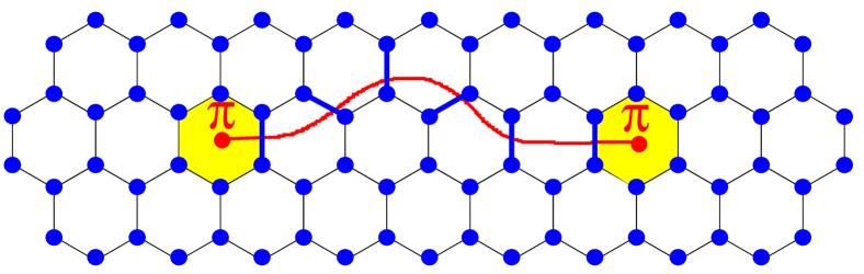
Figure 2: The illustration of the two $\pi$-flux (yellow plaquette) on the honeycomb lattice. When the fermion hops across the red strings which connect two fluxes, the wave function changes sign.

Firstly, we consider the TI with two well separated $\pi$-fluxes (for example, the distance between two fluxes is $5\sqrt{3}a$). See the illustration in Fig.2. The Hamiltonian in Eq.(1) then becomes

$$\hat{H}_{\mathrm{KM}}=-\mathit{T}\sum_{\left\langle i,j\right\rangle}\hat{c}_{i}^{\dagger}\epsilon_{ij}\hat{c}_{j}-\mathit{T}^{\prime}\sum\limits_{\left\langle\left\langle{i,j}\right\rangle\right\rangle}e^{i\phi_{ij}}\hat{c}_{i}^{\dagger}\epsilon_{ij}\hat{c}_{j}-\mu\sum_{i}\hat{c}_{i}^{\dagger}\hat{c}_{i}.$$ (4)

Here, $\epsilon_{ij}$ is $-1$ where the $\left\langle i,j\right\rangle$ link and $\left\langle\left\langle{i,j}\right\rangle\right\rangle$ link cross the red string which connects two fluxes shown in Fig.2, and otherwise, $\epsilon_{ij}$ is $1$.

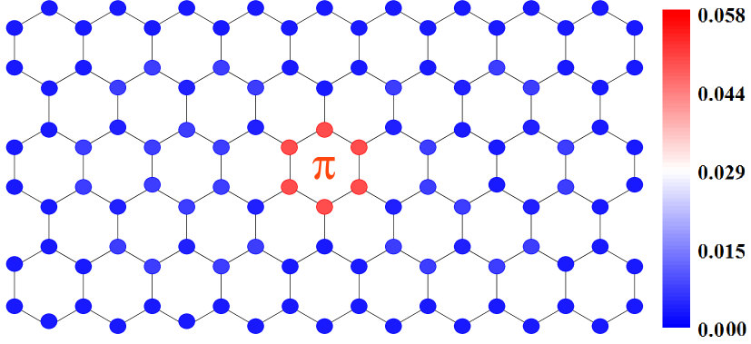
Figure 3: The illustration of the particle density distribution of fermionic zero modes when two fluxes are well separated. The color of dots denotes the probability of the particle on the lattice sites. The related parameters in Eq.(1) are chosen as $\mathit{T}=1.0$, $\mathit{T}^{\prime}=0.1$.

By using the exact diagonalization numerical approach on a $72\times 72$ lattice, we find that there exists fermionic zero mode around each $\pi$-flux. See the particle density around a $\pi$-flux in Fig.3. One can see that the particle density is mainly localized around the $\pi$-flux. The length-scale of the wave-function of the zero mode is $\xi\sim v_{F}/\Delta_{f}$ where $v_{F}=3a\mathit{T}/2$ is the Fermi velocity. When there are two fluxes nearby, the inter-flux quantum tunneling effect occurs and the two zero modes couple.

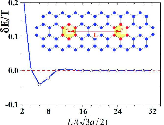
Figure 4: The energy splitting $\delta E$ versus the flux-distance $L$ for the case of $\mathit{T}=1.0$, $\mathit{T}^{\prime}=0.1$. $a$ is honeycomb lattice constant. The inset illustrates two $\pi$-flux with the flux-distance $L$.

As shown in Fig.4, the energy splitting $\delta E$ between two energy levels versus the flux-distance $L$, oscillates and decreases exponentially. When two fluxes are well separated, the quantum tunneling effect can be ignored and we have two quantum states with zero energy. On the other hand, for the small $L$, the coupling between zero modes becomes stronger and the energy splitting can not be neglected.

III.2 Mid-gap states of the Haldane model with triangular flux-superlattice

We next study the TI with a triangular flux-superlattice.

At the first step, by using the numerical calculations, we obtain the DOS for the Haldane model with a triangular flux-superlattice. See numerical results in Fig.5(b) with flux-superlattice constant $L=3\sqrt{3}a$ for the case of $\mathit{T}=1.0$, $\mathit{T}^{\prime}=0.1$. From Fig.5(b), one may see that the mid-gap bands appear. In Fig.5(c), the mid-gap bands in Fig.5(b) are zoomed in. Now, we find that there exist four points with van Hove singularity, and the mid-gap bands also have an energy gap.

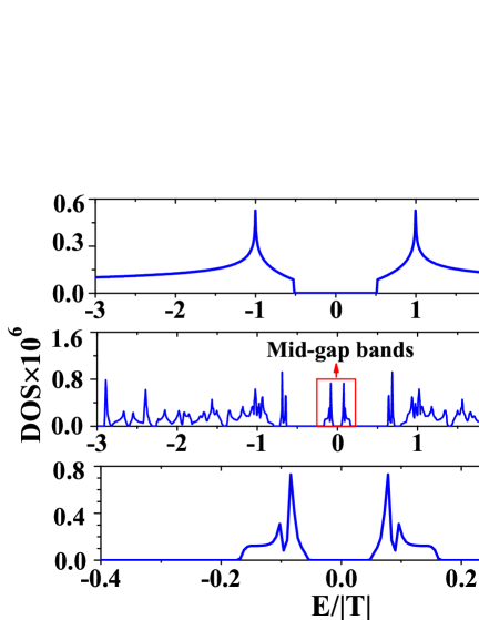
Figure 5: (a) The DOS of Haldane model without flux-superlattice for the case of $\mathit{T}=1.0$, $\mathit{T}^{\prime}=0.1$. (b) The DOS of TI with triangular flux-superlattice: the mid-gapped states are induced by the flux-superlattice with flux-superlattice constant $L=3\sqrt{3}a$ for the case of $\mathit{T}=1.0$, $\mathit{T}^{\prime}=0.1$. (c) The illustration of details of the mid-gap band in (b).

At second step, to illustrate the topological properties of the mid-gap states induced by the flux-superlattice of the parent TI, we study the edge states of the TI with flux-superlattice for the case of $\mathit{T}=1.0$, $\mathit{T}^{\prime}=0.1.$ We put the Haldane model with a finite flux-superlattice along x-direction on a torus. See the illustration in Fig.6(a). The parent topological insulator has the periodic boundary condition along both x-direction and y-direction. While the flux-superlattice has periodic boundary condition along y-direction and open boundary condition along x-direction. See the numerical results in Fig.6(b). There exist the edge states along the boundaries of the flux-superlattice. In addition, we plot the particle density distribution of the edge states in Fig.6(a). The existence of the gapless zero modes on the boundary of the flux-superlattice indicate the mid-gap system is indeed an induced ”topological insulator” on the parent TI.

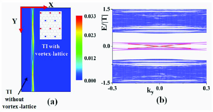
Figure 6: (a) The illustration of particle density of edge states along the boundaries of flux-superlattice. The flux-superlattice constant is $3\sqrt{3}a$. Related parameter is chosen as $\mathit{T}^{\prime}/\mathit{T}=0.1$; (b) The edge states of the composite system, of which the parent Haldane model has periodic boundary along both x and y directions, and while the flux-superlattice has periodic boundary along y direction and open boundary condition along x direction. Parameters (flux-superlattice constant, $\mathit{T}^{\prime}$, and $\mathit{T}$) are the same as given in (a).

IV Effective flux-superlattice model for the mid-gap states

In this section, we will write down an effective tight-binding model to describe the mid-gap states.

IV.1 Effective flux-superlattice model

The quantum states of the fermionic zero mode around a $\pi$-flux can be formally described in terms of the fermion Fock states $\left\{\left|0\right\rangle,\left|1\right\rangle\right\}$. Here, $\left|0\right\rangle,\left|1\right\rangle$ denote the un-occupied state and the occupied state, respectively. These quantum states are localized around the flux within a length-scale $\xi\sim v_{F}/\Delta_{f}$. For the case of $\xi<L$, we can consider each flux as an isolated ”atom” with localized electronic states and use the effective tight-binding model to describe these quantum states on the fluxes.

Now, we superpose the localized states to obtain the sets of Wannier wave functions $w(R)$ with $R$ denoting the position of the flux. Due to the formation of the triangular flux-superlattice, both the quantum-tunneling-strength $\delta E$ between NN fluxes and the quantum-tunneling-strength $\delta E^{\prime}$ between NNN fluxes exist. The ratio $\delta E^{\prime}/\delta E$ versus NN flux-superlattice constant $L$ is shown in Fig.7. Owing to the inter-flux quantum tunneling effect, we get energy splitting $\left|\delta E_{RR^{\prime}}\right|$ which is just the particle’s hopping amplitude $\left|t_{RR^{\prime}}\right|$ between two localized states on two $\pi$-fluxes at $R$ and $R^{\prime}$. Then the effective tight-binding model of the two fermionic zero modes takes the form of $t_{RR^{\prime}}\left(\hat{\alpha}_{R}^{\dagger}\hat{\alpha}_{R^{\prime}}+h.c.\right)$ with $\left|t_{RR^{\prime}}\right|=\left|\delta E_{RR^{\prime}}\right|$. With considering the NN and NNN hoppings, the effective tight-binding model of the localized states around the triangular flux-superlattice is given by

$$\hat{H}_{\mathrm{VL}}=-\sum_{\left\langle R,R^{\prime}\right\rangle}t_{RR^{\prime}}\hat{\alpha}_{R}^{\dagger}\hat{\alpha}_{R^{\prime}}-\sum_{\left\langle\left\langle R,R^{\prime}\right\rangle\right\rangle}t_{RR^{\prime}}^{\prime}\hat{\alpha}_{R}^{\dagger}\hat{\alpha}_{R^{\prime}},$$ (5)

where $\hat{\alpha}_{R}$ is the fermionic annihilation operator of a localized state on a flux $R$, and $t_{RR^{\prime}}$ ($t_{RR^{\prime}}^{\prime}$) is the hopping parameter between NN (NNN) sites $R$ and $R^{\prime}$. The NN (NNN) hopping term is denoted as $\left|t_{RR^{\prime}}\right|=t=\left|\delta E^{\prime}\right|$ ($\left|t_{RR^{\prime}}^{\prime}\right|=\left|\delta E^{\prime}\right|$). See the illustration in the inset of Fig.7. In particular, owing to the polygon rule (Each fermion gains an accumulated phase shift $\left|\phi\right|=(n-2)\pi/2$ encircling around a smallest n-polygonrule ), the total phase around each plaquette of the triangular flux-lattice is $\pm\frac{\pi}{2}$ for fermions. For example, we may choose the gauge as shown in Fig.8.

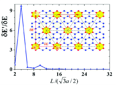
Figure 7: The ratio between the NNN quantum tunneling and the NN quantum tunneling ($\delta E/\delta E^{\prime}$) via flux-superlattice constant $L$, where $\delta E$ versus $L$ is shown in Fig.4. The inset shows triangular flux-superlattice. The tunnelings $\delta E$, $\delta E^{\prime}$ and the flux-superlattice constant $L$ are all indicated in the inset.

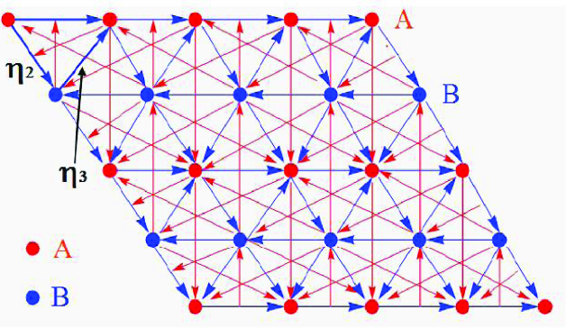
Figure 8: The illustration of the gauge choice. Moving along the arrow (both blue arrow and red arrow), the fermion acquires a phase shift $\pi/2.$ The accumulated phase encircling each triangular lattice plaquette anti-clockwise is $\pi/2$.

The ratio between the NN hopping strength $t$ and the NNN hopping strength $t^{\prime}$ is indeed the same as the ratio between $\left|\delta E\right|$ and $\left|\delta E^{\prime}\right|$. Because people can tune $\left|\delta E^{\prime}\right|/\left|\delta E\right|$ ($t^{\prime}/t$) by changing the flux-superlattice constant $L$ (see the results in Fig.7), we may regard the flux-superlattice model of the mid-gap states as an emergent controllable topological system.

IV.2 Topological properties

According to the gauge shown in Fig.8, we choose $t_{RR^{\prime}}=\mathrm{i}t$, $t_{RR^{\prime}}^{\prime}=\mathrm{i}t^{\prime}$ if fermions hop along directions of arrows. Now we label the fermionic annihilation operators of the localized states on the two sub-flux-superlattices by $\hat{A}_{R},$ $\hat{B}_{R}$. See Appendix A for the detailed formula of Eq.(5) in terms of operators $\hat{A}_{R}$, $\hat{B}_{R}$. By the Fourier transformation, we obtain the effective Hamiltonian of the tight-binding model of the TI with triangular flux-superlattice in momentum space as

$$\hat{H}_{\mathrm{VL}}=\sum_{k}\hat{\Phi}_{k}^{\dagger}\mathcal{H}_{k}\hat{\Phi}_{k},$$ (6)

where $\hat{\Phi}_{k}=\left(\begin{array}[c]{cc}\hat{A}_{k}&\hat{B}_{k}\end{array}\right)^{T}$ and $\mathcal{H}_{k}=\left(\mathbf{h}\cdot\mathbf{\tau}\right)$ with $\mathbf{h}=\left(h_{x},\text{ }h_{y},\text{ }h_{z}\right)$, and $\mathbf{\tau}$ the Pauli matrix. The three components of $\mathbf{h}$ are

$$h^{x} =2t\sin\left(\mathbf{k}\cdot\mathbf{\eta}_{2}\right)-2t^{\prime}\sin\left[\mathbf{k}\cdot\left(\mathbf{\eta}_{1}+\mathbf{\eta}_{3}\right)\right],$$

$$h^{y} =-2t\cos\left(\mathbf{k}\cdot\mathbf{\eta}_{3}\right)-2t^{\prime}\cos\left[\mathbf{k}\cdot\left(\mathbf{\eta}_{1}+\mathbf{\eta}_{2}\right)\right],$$

$$h^{z} =2t\sin\left(\mathbf{k}\cdot\mathbf{\eta}_{1}\right)-2t^{\prime}\sin\left[\mathbf{k}\cdot\left(\mathbf{\eta}_{2}-\mathbf{\eta}_{3}\right)\right],$$ (7)

where $\mathbf{\eta}_{1}=L\left(1,\text{ }0\right)$, $\mathbf{\eta}_{2}=L(\frac{1}{2},$ $-\frac{\sqrt{3}}{2}),$ $\mathbf{\eta}_{3}=L(\frac{1}{2},$ $\frac{\sqrt{3}}{2}).$ In the following, for simplicity, we set the flux-superlattice constant to be $L\equiv 1$. Then energy spectrums of the effective tight-binding model of the TI with triangular flux-superlattice are obtained as

$$E_{\mathrm{VL}}(\mathbf{k})=\pm\left|\mathbf{h}\right|=\pm\sqrt{(h^{x})^{2}+(h^{y})^{2}+(h^{z})^{2}}.$$ (8)

The topological quantum phase transition occurs when the band gap closes $E_{\mathrm{VL}}(\mathbf{k})=0$. See Fig.9(a). We find that there exists a quantum critical point at $t^{\prime}/t=1$ that separates two quantum phases, $0<t^{\prime}/t<1,$ $t^{\prime}/t>1$. To characterize the two quantum phases, we introduce the Chern numberdj

$$C=\frac{1}{4\pi}\int\text{{tr}}(\mathbf{n\cdot}\frac{\partial\mathbf{n}}{\partial k_{x}}\times\frac{\partial\mathbf{n}}{\partial k_{y}})d^{2}\mathbf{k},$$ (9)

with $\mathbf{n}=\mathbf{h/}\left|\mathbf{h}\right|$. According to the Chern number, we find that in the region of $0<t^{\prime}/t<1,$ the Chern number is $1$, and in the region of $t^{\prime}/t>1,$ the Chern number is $-3$. The tight-binding model of the TI with triangular flux-superlattice always has nontrivial topological properties. As a result, we call it topological flux-superlattice model that can describe the mid-gap states of the Haldane model with triangular flux-superlattice.

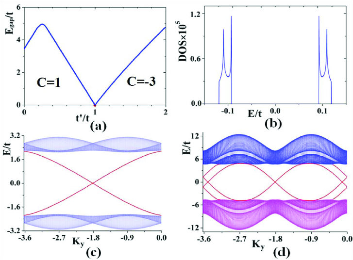
Figure 9: (a) The topological phases versus $t^{\prime}/t$; (b) The density of state of the free flux-lattice model. The parameters are chosen as $t/\mathit{T}=0.04,$ $t^{\prime}/\mathit{T}=0.014$; (c) The edge states of the tight-binding model of flux-superlattice for the case of $t^{\prime}=0.1t,$ in which the Chern-number is $C=1$; (d) The edge states of the tight-binding model of flux-superlattice for the case of $t^{\prime}=3.1t,$ in which the Chern-number is $C=-3$.

Next, we study the topological properties in different phases. In Fig.9(b) we show the DOS of the flux-superlattice model for the case of $t/\mathit{T}=0.04,$ $t^{\prime}/\mathit{T}=0.014$. From the DOS, we can see that the effective flux-superlattice model has a finite energy gap and there exist four points with van Hove singularity. Fig.9(c) and Fig.9(d) show the edge states for the case of $t^{\prime}=0.1t$ (the Chern-number is $C=1$) and $t^{\prime}=3.1t$ (the Chern-number is $C=-3$), respectively.

IV.3 Comparison between the effective flux-superlattice model and mid-gap system of the parent TI

The DOS of the Haldane model with triangular flux-superlattice is shown in Fig.5(b). Besides the gapped states of the parent Haldane model, there exist mid-gap states in the energy band gap. It is obvious that the mid-gap states are induced by the flux-superlattice. The mid-gap states have an energy gap and there also exist four points with van Hove singularity. In addition, the gapless edge states of the mid-gap states are shown in Fig.6(b). Correspondingly, using parameters $t$, $t^{\prime}$ derived from the flux-superlattice for the case of $L=3\sqrt{3}a$, we also get the gapless edge states of the effective flux-superlattice model, which are similar to those given in Fig.6(b).

Hence, the low energy physics of the Haldane model with flux-superlattice can be described by an effective flux-superlattice model. The effective flux-superlattice model shows nontrivial topological properties, including nontrivial topological invariant, gapless edge states. In this sense, the effective flux-superlattice model is really an emergent ”topological insulator” on the parent TIs. The situation is much different from the TI with a flux-line discussed in Ref.Assaad , of which the mid-gap states of a TI with a flux-line has no nontrivial topological properties.

V Conclusions and discussions

In this paper we mainly studied the Haldane model with triangular flux-superlattice. We found that there exist the mid-gap states with nontrivial topological properties, including the nonzero Chern number and the gapless edge states. We wrote down an effective tight-binding model (the effective flux-superlattice model) to describe the mid-gap states. Using similar approach, we studied the Haldane model with other types of flux-superlattices such as the square flux-superlattice and honeycomb flux-superlattice, and find similar topological properties. In this sense, the topological mid-gap states always exist in a TI with flux-superlattices.

In addition, we need to point out that the Kane-Mele modelkane2 or the spinful Haldane modelhe with flux-superlattice exhibit similar topological features. Due to the spin degree of freedom, a $\pi$-flux on the these models traps two zero models. The overlap of zero modes also gives rise to a topological mid-gap system inside the band gap of parent TIs. When one considers the interaction between the two-component fermions, the topological mid-gap system may lead to quite different physics consequences. These issues are beyond the discussion in this paper and will be studied elsewhere.

Appendix A Effective flux-superlattice model of the TI with triangular flux-superlattice

The Hamiltonian for the effective flux-superlattice model of the TI with triangular flux-superlattice is given by

$$\hat{H}=\hat{H}_{\mathrm{NN}}+\hat{H}_{\mathrm{NNN}},$$ (10)

where $\hat{H}_{\mathrm{NN}}$ ($\hat{H}_{\mathrm{NNN}}$) denotes the NN (NNN) hopping term, respectively. The gauge is chosen as shown Fig.8. The detailed formulas of $\hat{H}_{\mathrm{NN}}$ and $\hat{H}_{\mathrm{NNN}}$ are explicitly written as

$$\hat{H}_{\mathrm{NN}} =\hat{H}_{\mathrm{NN}}^{\mathrm{A}}+\hat{H}_{\mathrm{NN}}^{\mathrm{B}},$$ (11)

$$\hat{H}_{\mathrm{NNN}} =\hat{H}_{\mathrm{NNN}}^{\mathrm{A}}+\hat{H}_{\mathrm{NNN}}^{\mathrm{B}},$$ (12)

with

$$\hat{H}_{\mathrm{NN}}^{\mathrm{A}}=it\sum_{R}\left(-A_{R}^{\dagger}A_{R+\mathbf{\eta}_{1}}+A_{R}^{\dagger}B_{R+\mathbf{\eta}_{3}}+A_{R}^{\dagger}B_{R-\mathbf{\eta}_{2}}+A_{R}^{\dagger}A_{R-\mathbf{\eta}_{1}}+A_{R}^{\dagger}B_{R-\mathbf{\eta}_{3}}-A_{R}^{\dagger}B_{R+\mathbf{\eta}_{2}}\right)$$ (13)

$$\hat{H}_{\mathrm{NN}}^{\mathrm{B}}=it\sum_{R}\left(B_{R}^{\dagger}B_{R+\mathbf{\eta}_{1}}-B_{R}^{\dagger}A_{R+\mathbf{\eta}_{3}}+B_{R}^{\dagger}A_{R-\mathbf{\eta}_{2}}-B_{R}^{\dagger}B_{R-\mathbf{\eta}_{1}}-B_{R}^{\dagger}A_{R-\mathbf{\eta}_{3}}-B_{R}^{\dagger}A_{R+\mathbf{\eta}_{2}}\right)$$ (14)

$$\hat{H}_{\mathrm{NNN}}^{\mathrm{A}}=it^{\prime}\sum_{R}\left(A_{R}^{\dagger}B_{R+\mathbf{\eta}_{1}+\mathbf{\eta}_{3}}-A_{R}^{\dagger}A_{R-\mathbf{\eta}_{2}+\mathbf{\eta}_{3}}+A_{R}^{\dagger}B_{R-\mathbf{\eta}_{1}-\mathbf{\eta}_{2}}-A_{R}^{\dagger}B_{R-\mathbf{\eta}_{1}-\mathbf{\eta}_{3}}+A_{R}^{\dagger}A_{R+\mathbf{\eta}_{2}-\mathbf{\eta}_{3}}+A_{R}^{\dagger}B_{R+\mathbf{\eta}_{1}+\mathbf{\eta}_{2}}\right)$$ (15)

$$\hat{H}_{\mathrm{NNN}}^{\mathrm{B}}=it^{\prime}\sum_{R}\left(B_{R}^{\dagger}A_{R+\mathbf{\eta}_{1}+\mathbf{\eta}_{3}}+B_{R}^{\dagger}B_{R-\mathbf{\eta}_{2}+\mathbf{\eta}_{3}}-B_{R}^{\dagger}A_{R-\mathbf{\eta}_{1}-\mathbf{\eta}_{2}}-B_{R}^{\dagger}A_{R-\mathbf{\eta}_{1}-\mathbf{\eta}_{3}}-B_{R}^{\dagger}B_{R+\mathbf{\eta}_{2}-\mathbf{\eta}_{3}}-B_{R}^{\dagger}A_{R+\mathbf{\eta}_{1}+\mathbf{\eta}_{2}}\right)$$ (16)

References

- (1) F. D. M. Haldane, Phys. Rev. Lett. 61, 2015 (1988).
- (2) C. L. Kane and E. J. Mele, Phys. Rev. Lett. 95, 226801 (2005).
- (3) C. L. Kane and E. J. Mele, Phys. Rev. Lett. 95, 146802 (2005).
- (4) B. A. Bernevig, T. L. Huge and S. C. Zhang, Science 314, 1757 (2006).
- (5) Y. Ran, A. Vishwanath, and D. H. Lee, Phys. Rev. Lett. 101, 086801 (2008).
- (6) X. L. Qi and S. C. Zhang, Phys. Rev. Lett. 101, 086802 (2008).
- (7) F. F. Assaad, M. Bercx, and M. Hohenadler, Phys. Rev. X 3, 011015 (2013).
- (8) V. Lahtinen, A. W. Ludwig, J. K.Pachos, and S. Trebst, Phys. Rev. B 86, 075115 (2012).
- (9) J. Zhou, Y. J. Wu, R. L. Wu, S. P. Kou, EPL, 102, 47005 (2013).
- (10) D. J. Thouless, M. Kohmoto, P. Nightingale, and M. den Nijs, Phys. Rev. Lett. 49, 405 (1982).
- (11) J. Avron, R. Seiler, and B. Simon, Phys. Rev. Lett. 51, 51 (1983).
- (12) E. Grosfeld and Ady Stern, Phys. Rev. B 73, 201303 (2006).
- (13) D. N. Sheng, Z. Y. Weng, L. Sheng, and F. D. M. Haldane, Phys. Rev. Lett. 97, 036808 2006.
- (14) J. He, S.P. Kou, Y. Liang, S.P. Feng, Phys. Rev. B 83, 205116 (2011).