Heralded single phonon preparation, storage and readout in cavity optomechanics

Abstract

We show how to use the radiation pressure optomechanical coupling between a mechanical oscillator and an optical cavity field to generate in a heralded way a single quantum of mechanical motion (a Fock state). Starting with the oscillator close to its ground state, a laser pumping the upper motional sideband produces correlated photon-phonon pairs via optomechanical parametric downconversion. Subsequent detection of a single scattered Stokes photon projects the macroscopic oscillator into a single-phonon Fock state. The non-classical nature of this mechanical state can be demonstrated by applying a readout laser on the lower sideband to map the phononic state to a photonic mode, and performing an autocorrelation measurement. Our approach proves the relevance of cavity optomechanics as an enabling quantum technology.

Introduction

Cavity optomechanical systems consist of a mechanical oscillator at frequency $\Omega_{m}/2\pi$ coupled to an electromagnetic cavity mode with resonant frequency $\omega_{c}/2\pi$ Aspelmeyer et al. (2013) (Fig. 1a). The radiation pressure optomechanical coupling can be used to either amplify Kippenberg and Vahala (2008) or cool Arcizet et al. (2006); Schliesser et al. (2006); Gigan et al. (2006); Wilson-Rae et al. (2007); Marquardt et al. (2007); Schliesser et al. (2009) the mechanical degree of freedom. This has enabled the preparation of mechanical oscillators in the quantum regime O’Connell et al. (2010); Teufel et al. (2011); Chan et al. (2011); Safavi-Naeini et al. (2012) and the quantum coherent coupling between light and mechanical degrees of freedom Verhagen et al. (2012); Palomaki et al. (2013a). Likewise, the optomechanical interaction allows for the readout of mechanical motion with a readout imprecision below that at the standard quantum limit Teufel et al. (2009); Anetsberger et al. (2010). In addition, optomechanically induced transparency Weis et al. (2010) can be utilized for slowing or advancing electromagnetic signals Safavi-Naeini et al. (2011); Zhou et al. (2013), for coherent transfer between two optical wavelengths Hill et al. (2012), between the microwave and optical domains Bochmann et al. (2013); Andrews et al. (2013), and for information storage and retrieval in long-lived oscillations Palomaki et al. (2013a); Fiore et al. (2011); McGee et al. (2013).

In the context of quantum information, continuous-variable schemes Schmidt et al. (2012) such as optomechanical squeezing Vanner et al. (2013a); Szorkovszky et al. (2013) and entanglement Palomaki et al. (2013b) in the quadrature operators have been demonstrated in recent experiments. Yet there are many advantages to using discrete variables, for which heralded probabilistic protocols can exhibit very high fidelity and loss-resilience Sangouard et al. (2011). Moreover, on a fundamental level, studying quantized energy eigenstates of macroscopic objects may allow new tests of quantum mechanics Pepper et al. (2012) and of the nature of entanglement Pirandola et al. (2006); Børkje et al. (2011); Lee et al. (2011). The first step toward this goal is to generate single-phonon Fock states in long lived mechanical oscillators.

One possible route is to break the harmonicity of the system’s eigenstates by reaching the single-photon strong coupling regime Rabl (2011); Nunnenkamp et al. (2011); Rips et al. (2012); Ludwig et al. (2012); Liao and Nori (2013); Qiu et al. (2013); Kronwald et al. (2013); Rips and Hartmann (2013); Xu et al. (2013a, b), or to use the nonlinearity resulting from coupling to two level systems Stannigel et al. (2012); Ramos et al. (2013). However, the former requires $g_{0}/(\kappa,\varOmega_{m})\gtrsim 1$, where $g_{0}$ is the single-photon optomechanical coupling rate (see below) and $\kappa$ is the total cavity energy decay rate $-$ a regime far from state of the art experiments where $g_{0}/\kappa\sim 10^{-3}$ Verhagen et al. (2012); Chan et al. (2012). If multiple optical modes are introduced a non conventional photon blockade regime can be used to relax the constraint on the coupling strength Xu and Li (2013); Savona (2013) $-$ and has been recently considered for conditional preparation of non-classical states Basiri-Esfahani et al. (2012); Kómár et al. (2013). Projective measurements have also been proposed by Vanner et al. to realize phonon addition and subtraction operations for general quantum state orthogonalization Vanner et al. (2013b).

In this Letter, we present an approach based on single-photon detection to generate a single-phonon Fock state in a heralded way and then convert it into a single photon, in the experimentally relevant weak-coupling and resolved-sideband Wilson-Rae et al. (2007); Marquardt et al. (2007) regime of a single-mode optomechanical system (Figs. 1a-d). Starting with the mechanical mode close to its ground state (mean phonon number $\bar{n}_{0}\ll 1$), a write laser pulse, tuned to the upper motional sideband of the optical cavity, is used to amplify Kippenberg et al. (2005) the mechanical motion and generate (with low probability) a correlated photon-phonon pair via optomechanical parametric downconversion. The scattered photon $-$ referred to as Stokes photon in the following $-$ is spectrally-filtered from the pump and detected by a photon counting module, thereby projecting the mechanical oscillator (from its weak coherent state) into a single-phonon Fock state while heralding the success of the procedure Vanner et al. (2013b). To verify the non-classical nature of the heralded mechanical state, the mechanical excitation is coherently mapped onto the optical cavity field by applying a readout laser tuned to the lower mechanical sideband (corresponding to resolved sideband cooling Schliesser et al. (2009)), and the statistics of these Anti-Stokes photons is analyzed in an autocorrelation ($g^{(2)}$) measurement Kimble et al. (1977); Grangier et al. (1986). In the limit where the write (amplifying) and readout (cooling) pulses are shorter than the mechanical decoherence time, and for a small enough initial phonon occupancy ($\bar{n}_{0}\ll 1$), the two-fold coincidence probability vanishes ($g^{(2)}\rightarrow 0$) (Fig. 1d), demonstrating the heralded creation of a single-phonon Fock state and its successful upconversion into a single cavity photon.

Principle.

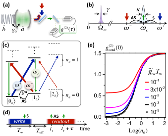
Figure 1: (a) Schematics of the optomechanical system pumped at the upper and lower motional sidebands and of the correlation measurement on the filtered cavity photons. (b) Representation of the relevant mechanical and optical frequencies and linewidths. (c) Resonant transitions during the write and readout pulses. For a given mean photon number $n_{a}$ the number (Fock) states of the mechanical oscillator form a harmonic ladder. Emission at $\omega_{c}$ is enhanced by the cavity, which allows to address selectively the Stokes, S (resp. anti-Stokes, AS) transitions between phonon states when driving the upper (resp. lower) mechanical sideband. (d) Pulse sequence (cooling step not shown). Detection of a Stokes photon within the write pulse duration $T_{\text{w}}$ is the heralding event. After a storage time $T_{\text{off}}$, coincidences between anti-Stokes photons emitted at time $t_{\text{r}}$ and $t_{\text{r}}+\tau$ are measured. We define $t_{\text{r}}=0$ at the beginning of the readout pulse. (e) Conditional two-photon coincidence as a function of the initial mechanical occupancy $\bar{n}_{0}$ (log scale) for different values of the product $\widetilde{g}_{\text{w}}T_{\text{w}}$, under the assumption of negligible mechanical damping ($T_{\text{w}}\ll(\gamma\bar{n}_{\text{th}})^{-1}$ and $T_{\text{off}}=0$). Open squares: only single-photon emission events are post-selected, eq.(5). Solid lines: including the contribution from multiple photon emission.

We consider the optical and mechanical modes (represented by bosonic operators $\hat{a}$ and $\hat{b}$, respectively) of an optomechanical cavity driven by a laser on the lower or upper mechanical sideband, corresponding to the angular frequencies $\omega_{\pm}=\omega_{c}\pm\Omega_{m}$ (Fig. 1b). The Hamiltonian is a sum of three terms $\hat{\mathcal{H}}=\hat{\mathcal{H}}_{0}+\hat{\mathcal{H}}_{OM}+\hat{\mathcal{H}}_{dr\pm}$ describing the uncoupled systems, $\hat{\mathcal{H}}_{0}=\hbar\omega_{c}\hat{a}^{{\dagger}}\hat{a}+\hbar\Omega_{m}\hat{b}^{{\dagger}}\hat{b}$; the optomechanical interaction, $\hat{\mathcal{H}}_{OM}=-\hbar g_{0}\hat{a}^{{\dagger}}\hat{a}(\hat{b}^{{\dagger}}+\hat{b})$; and the laser driving, $\hat{\mathcal{H}}_{dr\pm}=\hbar(s_{\pm}^{*}e^{i\omega_{\pm}t}\hat{a}+s_{\pm}e^{-i\omega_{\pm}t}\hat{a}^{{\dagger}})$, where $|s_{\pm}|=\sqrt{\kappa P_{\pm}/\hbar\omega_{\pm}}$ is the incoming photon flux for a laser power $P_{\pm}$. As detailed in , after switching to the interaction picture with respect to $\hat{\mathcal{H}}_{0}$ and taking the weak-coupling ($g_{0}\ll\kappa$) and resolved-sideband ($\kappa\ll\Omega_{m}$) limits we obtain the linearized Langevin equations during the write (amplification) pulse

$$\frac{d\hat{a}}{dt} =\frac{i}{\hbar}[\hat{\mathcal{H}}_{BSB},\hat{a}]-\frac{\kappa}{2}\hat{a}+\sqrt{\kappa}\hat{a}_{\text{in}}$$ (1a)

$$\frac{d\hat{b}}{dt} =\frac{i}{\hbar}[\hat{\mathcal{H}}_{BSB},\hat{b}]-\frac{\gamma}{2}\hat{b}+\sqrt{\gamma}\hat{b}_{\text{in}}$$ (1b)

with $\gamma$ the energy decay rate of the mechanical oscillator. $\hat{\mathcal{H}}_{BSB}=-\hbar g_{+}\hat{a}^{{\dagger}}\hat{b}^{{\dagger}}+h.c$ is a parametric gain interaction and leads to the generation of photon-phonon pairs (Fig. 1c). Here $g_{+}=g_{0}\sqrt{\bar{n}_{\text{w}}}$ is the effective optomechanical coupling rate enhanced by the intracavity photon number $\bar{n}_{\text{w}}=|\frac{-is_{+}}{-i\Omega_{m}+\kappa/2}|^{2}=\frac{\kappa P_{+}}{\hbar\omega_{c}(\Omega_{m}^{2}+\kappa^{2}/4)}$ at the laser frequency. For simplicity we consider the optical cavity to be overcoupled, i.e. the total cavity decay rate is dominated by the external in/out-coupling rate $\kappa_{\text{ext}}$, so that $\kappa\simeq\kappa_{\text{ext}}$. The operator $\hat{a}_{\text{in}}$ represents the vacuum noise entering the optical cavity, and $\hat{b}_{\text{in}}$ is the thermal noise from a phonon bath at temperature $T_{\text{bath}}$ and mean occupancy $\bar{n}_{\text{th}}\approx\frac{k_{B}T_{\text{bath}}}{\hbar\Omega_{m}}$. The oscillator initial thermal occupancy $\bar{n}_{0}$ can be significantly smaller than $\bar{n}_{th}$ if the readout laser is also used for sideband cooling (see Sec. III in SM) Schliesser et al. (2009); Chan et al. (2011).

In a first simplified treatment, we neglect the decay of the mechanical oscillator, which is a valid approximation if the pulse sequence is shorter than the thermal decoherence time $(\gamma\bar{n}_{\text{th}})^{-1}$. Since in our scheme $g_{+}\ll\kappa$, we can adiabatically eliminate the cavity mode in eqs.(1a,1b) $\hat{a}_{\text{w}}(t)\simeq\frac{2}{\kappa}(ig_{+}\hat{b}_{\text{w}}^{{\dagger}}+\sqrt{\kappa}\hat{a}_{\text{w,in}})$. Using the input/output relations Gardiner and Collett (1985) $\hat{a}_{\text{w,out}}=-\hat{a}_{\text{w,in}}+\sqrt{\kappa}\hat{a}_{\text{w}}$ (the subscript w refers to the operators during the write pulse) we obtain the coupled optomechanical equations

$$\hat{a}_{\text{w,out}} =\hat{a}_{\text{w,in}}+i\sqrt{2\tilde{g}_{\text{w}}}\hat{b}_{\text{w}}^{{\dagger}}$$ (2a)

$$\frac{d\hat{b}_{\text{w}}}{dt} =\tilde{g}_{\text{w}}\hat{b}_{\text{w}}+i\sqrt{2\tilde{g}_{\text{w}}}\hat{a}_{\text{w,in}}^{{\dagger}}$$ (2b)

where $\tilde{g}_{\text{w}}\equiv\frac{2g_{+}^{2}}{\kappa}$. Introducing the temporal modes Hofer et al. (2011) for the cavity driven by a write pulse of duration $T_{\text{w}}$, $\hat{A}_{\text{w,in/out}}(T_{\text{w}})=(\frac{\pm 2\tilde{g}_{\text{w}}}{1-e^{\mp 2\tilde{g}_{\text{w}}T_{\text{w}}}})^{-\frac{1}{2}}\int_{0}^{T_{\text{w}}}e^{\mp\tilde{g}_{\text{w}}t}\hat{a}_{\text{in/out}}(t)dt$, we can write the solutions of Eqs.(2a,2b) as $U^{{\dagger}}A_{\text{w,in}}U$ and $U^{{\dagger}}b_{\text{w}}(0)U$ where the propagator $U$ is given by

$$U(T_{\text{w}})=e^{i\sqrt{1-e^{-2\tilde{g}_{\text{w}}T_{\text{w}}}}\hat{A}_{\text{w,in}}^{{\dagger}}\hat{b}_{\text{w}}^{{\dagger}}}\\ e^{\tilde{g}_{\text{w}}T_{\text{w}}(-1-\hat{A}_{\text{w,in}}^{{\dagger}}\hat{A}_{\text{w,in}}-\hat{b}_{\text{w}}^{{\dagger}}\hat{b}_{\text{w}})}e^{-i\sqrt{1-e^{-2\tilde{g}_{\text{w}}T_{\text{w}}}}\hat{A}_{\text{w,in}}\hat{b}_{\text{w}}}$$ (3)

For an oscillator initially in a thermal state characterized by the density matrix $\rho_{b}(0)=(1-p)\sum_{n\geq 0}p^{n}|n\rangle\langle n|$ with $p\equiv\frac{\bar{n}_{0}}{1+\bar{n}_{0}}$ the state of the optomechanical system at the end of the write pulse is $\rho_{A,b}(T_{\text{w}})=U(T_{\text{w}})(|0_{A}\rangle\langle 0_{A}|\otimes\rho_{b}(0))U^{\dagger}(T_{\text{w}})$. The conditional mechanical state upon detection of a single photon in mode $\hat{A}_{\text{w,out}}$ is obtained by applying the projection operator $|1_{A}\rangle\langle 1_{A}|\otimes\mathbb{I}_{b}$, tracing out the optical mode and normalizing,

$$\rho_{b}^{\text{cond}}(T_{\text{w}}) =\frac{tr_{A}\>\{(|1_{A}\rangle\langle 1_{A}|\otimes\mathbb{I}_{b})\rho_{A,b}(T_{\text{w}})\}}{tr_{A,b}\>\{(|1_{A}\rangle\langle 1_{A}|\otimes\mathbb{I}_{b})\rho_{A,b}(T_{\text{w}})\}}$$

$$=(1-\overline{p})^{2}\sum_{n\geq 0}\overline{p}^{n}(n+1)|n+1\rangle\langle n+1|$$ (4)

where $\overline{p}=pe^{-\tilde{g}_{\text{w}}T_{\text{w}}}$. For a small gain parameter ($\tilde{g}_{\text{w}}T_{\text{w}}\ll 1$), which is essential to maximize the probability of successful single-phonon heralding (see ), and a resonator initially in its ground state ($p\ll 1$), the dominant term is the single-phonon Fock state $|1_{b}\rangle$.

In the readout step, driving the lower sideband at $\omega_{-}$ leads to the beam-splitter interaction $\hat{\mathcal{H}}_{RSB}=-\hbar g_{-}\hat{a}^{{\dagger}}\hat{b}+h.c$ (with $g_{-}=g_{0}\sqrt{\bar{n}_{\text{r}}}$ and $\bar{n}_{\text{r}}$ the intracavity photon number at the red sideband) replacing $\hat{\mathcal{H}}_{BSB}$ in Eqs.(1a,1b), which coherently swaps the optical and mechanical states (Fig. 1c). The phonon statistics can thus be mapped onto the anti-Stokes photons and subsequently be measured with a Hanbury-Brown Twiss setup (Fig. 1a) Kimble et al. (1977). Following similar steps as above, we compute the zero-delay second-order autocorrelation of the anti-Stokes photons during the readout pulse, $g_{\text{cond}}^{(2)}(0)=\frac{\langle\hat{A}_{\text{r,out}}^{{\dagger}2}\hat{A}_{\text{r,out}}^{2}\rangle_{c}}{\langle\hat{A}_{\text{r,out}}^{{\dagger}}\hat{A}_{\text{r,out}}\rangle_{c}^{2}}$, where the expectation value is taken on the post-selected mechanical state, eq.(4). We find

$$g_{\text{cond}}^{(2)}(0)=\frac{2\overline{p}(2+\overline{p})}{(1+\overline{p})^{2}}\approx 4\bar{n}_{0}$$ (5)

where the last approximation is valid in the limit $\bar{n}_{0}\ll 1$ and $\tilde{g}_{\text{w}}T_{\text{w}}\ll 1$. This result shows that the two-fold coincidence probability vanishes linearly with $\bar{n}_{0}$ and proves the non-classical nature of the heralded phonon state. In Fig. 1e we plot eq.(5) along with the results obtained when multiple photon emission is taken into account (see ) for different values of the gain parameter $\tilde{g}_{\text{w}}T_{\text{w}}$. We note that for sufficient readout laser power the internal phonon-to-photon conversion efficiency, approximated by $1-e^{-2\tilde{g}_{\text{r}}T_{\textrm{r}}}$ in the limit $p\ll 1$ ($\tilde{g}_{\text{r}},T_{\textrm{r}}$ are given explicitly in ), can be close to 1.

Let us briefly recall the conditions for observing strong antibunching: (i) Weak-coupling and resolved-sideband regime: $g_{0}\ll\kappa\ll\Omega_{m}$; (ii) Negligible mechanical decoherence: $T_{\text{w}}+T_{\text{off}}\ll(\gamma\bar{n}_{\text{th}})^{-1}$; and (iii) High initial occupancy of the ground-state: $\bar{n}_{0}\ll 1$. Because the pulse duration is bounded from below by $T_{\text{w}}>1/\kappa$ (the spectral width of the pulse should be narrower than the cavity), we can recast (ii) onto the condition: $\gamma\bar{n}_{\text{th}}\ll\kappa$. Noting that for a given bath temperature $\bar{n}_{\text{th}}\propto 1/\Omega_{m}$, this shows that the oscillator should have both a large $Q$ and a large frequency $\Omega_{m}$.

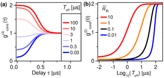
Figure 2: (a) Conditional second-order correlation function $g_{\text{cond}}^{(2)}(\tau|t_{\text{r}})$ at fixed $t_{\text{r}}=1$ ns for increasing waiting time $T_{\text{off}}$ between the write and readout pulses. The bath temperature is set to 1.6 K ($\bar{n}_{\text{th}}=6.4$). The transition from antibunching to bunching is a signature of the relaxation from a single-phonon Fock state to a thermal state. (b) Same-time correlation $g_{\text{cond}}^{(2)}(0)$ (i.e. two-photon emission probability) as a function of $T_{\text{off}}$ for decreasing phonon bath thermal occupancy $n_{\text{th}}$, yielding coherence times up to $(\gamma\bar{n}_{\text{th}})^{-1}\sim 100$ $\mu$s.

Experimental Feasibility.

Many optomechanical systems have already been demonstrated that satisfy (i) and for which condition (ii) would be trivially achieved owing to the typically long mechanical decay time Goryachev et al. (2012); Sun et al. (2012); Chakram et al. (2013) , but condition (iii) is challenging to meet in these systems. Here we consider a photonic crystal nanobeam resonator Kuramochi et al. (2010); Chan et al. (2011, 2012), for which the very high frequency of the confined phonon mode ($\Omega_{m}/2\pi\simeq 5$ GHz) is beneficial. For a given bath temperature, fewer quanta are thermally excited, while a large $\Omega_{m}$ also facilitates spectral filtering of the (anti-)Stokes photons from the pump laser beam (e.g. with high-Finesse Fabry-Perot filters). Moreover, the structures reported in Chan et al. (2012) exhibit large optomechanical coupling rate $g_{0}/2\pi\simeq 1$MHz and their optical linewidth $\kappa/2\pi<1$GHz place them in the resolved-sideband regime. Finally, coherence times of $\mathcal{O}(10-100\cdot 10^{-6}\text{\text{{s}}})$ are within reach at 4 K and below Sun et al. (2013) as mechanical energy decay rates of $\gamma/2\pi\simeq 7.5$ kHz have been measured at 10 K Chan et al. (2012).

Using the parameters reported in Chan et al. (2012) and a realistic bath temperature $T_{\text{bath}}\approx 1.6$ K (corresponding to He-4 buffer gas cooling Rivière et al. (2013)), an initial occupancy of $\bar{n}_{0}\approx 0.01$ can be achieved by 100 ns of sideband cooling with a peak intracavity photon number $\bar{n}_{\text{r}}=10^{3}$ corresponding to 150 $\mu$W of peak external laser power (see , Sec. III). The cooling laser is switched off during the write/store sequence. Including mechanical dissipation, we integrate eqs.(1a,1b) and compute $g_{\text{cond}}^{(2)}(\tau|t_{\text{r}})$, the probability for anti-Stokes photon emission at times $t_{\text{r}}$ and $t_{\text{r}}+\tau$ during the readout pulse, conditioned on the detection of a herald photon during the write pulse (see Fig. 1d). In Fig. 2a we plot $g_{\text{cond}}^{(2)}(\tau|t_{\text{r}}=1$ ns) for fixed write pulse parameters $T_{\text{w}}=50$ ns and $\bar{n}_{\text{w}}=0.1$, corresponding to a probability of Stokes emission $\sim 2\tilde{g}_{\text{w}}T_{\text{w}}(1+\bar{n}_{0})\sim 10^{-3}$/pulse. For waiting times between the write and readout pulses shorter than the decoherence time of the mechanics, $T_{\text{off}}\ll(\gamma\bar{n}_{\text{th}})^{-1}\simeq 20$ $\mu$s, we observe clear antibunching, a signature of successful conversion of the phonon Fock state into a single photon.

Beyond verifying the non-classical state of the macroscopic oscillator, our results also suggest a new tool for the on-demand generation of single photons Chou et al. (2004); Chen et al. (2006); Matsukevich et al. (2006). Within a time-window $\sim(\gamma\bar{n}_{\text{th}})^{-1}$ the heralded Fock state is stored in the mechanical oscillator and can be retrieved on-demand by applying the readout pulse.

Some advantageous features of the optomechanical systems considered here is that the single photons are emitted in a well-defined spatial mode and may be coupled into a single-mode fiber with high efficiency $>90\%$ Cohen et al. (2013); Gröblacher et al. (2013). Operation over the entire electromagnetic wavelength range and integration into large scale photonic circuits Streshinsky et al. (2013) are other appealing assets. By engineering a cavity supporting two optical modes both coupled to a same mechanical mode, one could generate the herald photon and release the readout photon at two arbitrary wavelengths. Although the write step is intrinsically probabilistic, it is possible to achieve near-deterministic Fock state creation by employing simple feedback techniques Felinto et al. (2006); Chen et al. (2006); Matsukevich et al. (2006).

Our scheme additionally enables precise control on the linewidth and coherence properties of the on-demand single photons Almendros et al. (2009) by tuning the strength of the readout pulse characterized by the peak intracavity photon number $\bar{n}_{\text{r}}$ (at the sideband $\omega_{-}$), as shown in Fig. 3. In the limit of weak readout laser ($\bar{n}_{\text{r}}\lesssim 1$) the anti-Stokes photon coherence time is set by the thermal coherence time of the oscillator $(\gamma\bar{n}_{\text{th}})^{-1}$. Increasing $\bar{n}_{\text{r}}$ shortens the coherence time and eventually we reach the (laser-enhanced) strong coupling regime $g_{-}\gtrsim\kappa$ and observe the onset of Rabi oscillations for $\bar{n}_{\text{r}}\gtrsim 10^{4}$, corresponding to multiple phonon-photon swapping cycles within the optical cavity lifetime. This yields a remarkable range of achievable coherence times, and therefore provides a way to generate on-demand single photons with tunable linewidths from tens of kHz to hundreds of MHz, an interesting feature for envisioned quantum networks, e.g. to couple various physical realizations of nodes using photons as carriers of quantum information.

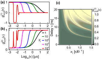
Figure 3: Shaping single photons (a) Field and (b) intensity two-time correlation as a function of the time delay $\tau$ between photons, for increasing readout pulse intracavity photon number $\bar{n}_{\text{r}}$ (from black to red). Bath temperature is 1.6 K and $T_{\text{off}}=5$ ns. The coherence time can be tuned over three orders of magnitude from $10$ $\mu$s down to $10$ ns, corresponding to linewidths from 100 kHz to 100 MHz. (c) Color plot of $g_{\text{cond}}^{(2)}(\tau)$ versus $\bar{n}_{\text{r}}$ and $\tau$. Rabi oscillations set in when the laser-enhanced optomechanical coupling becomes larger than the cavity decay rate: $g_{-}>\kappa$. Dashed lines show the expected maxima for the Rabi period $\frac{1}{2}\sqrt{g_{0}^{2}\bar{n}_{\text{r}}-\frac{1}{16}\kappa^{2}}$.

Entanglement and quantum repeaters.

The potential applications of optomechanical systems become more evident when noting the analogy with the scheme based on Raman transitions in atomic ensembles first proposed by Duan et al. Duan et al. (2001) to achieve scalable entanglement distribution between distant nodes (DLCZ protocol). Specifically, consider two distant optomechanical systems coherently excited by a weak laser beam, such that the probability that both systems are simultaneously excited is negligible. The resulting Stokes modes are interfered on a beamsplitter Børkje et al. (2011) and the detection of a single photon projects the distant mechanical oscillators into an entangled state where they share a single delocalized phonon. Successive entanglement swapping operations can then be used to extend the entanglement over hundreds of kilometers Sangouard et al. (2008).

As a quantitative example, let us estimate the average time $T_{\text{ent}}$ required to establish entanglement between two optomechanical resonators separated by 10 km of optical fiber using the DLCZ scheme. To first order in the small parameter $\tilde{g}_{\text{w}}T_{\text{w}}$ we have Sangouard et al. (2011); Sekatski et al. (2011): $T_{\text{ent}}\simeq(2R_{r}\cdot 2\tilde{g}_{\text{w}}T_{\text{w}}\cdot\eta)^{-1}$ where $R_{r}$ is the repetition rate of the experiment and $\eta$ the overall detection efficiency of the Stokes photons. For the particular system considered here, realistic values are $R_{r}=10$ MHz and $\eta=0.5\times 0.6\times 0.2=6\%$, where the three factors correspond, in this order, to the collection in a single-mode fiber, the propagation over 10 km of fibers, and the detection efficiency. Although $T_{\text{ent}}$ can be made shorter by increasing $\tilde{g}_{\text{w}}T_{\text{w}}$, this also increases the probability for multiple pair excitation and thereby decreases the fidelity expressed as $F\simeq(1-\bar{n}_{0})^{-1}(1-3\cdot 2\tilde{g}_{\text{w}}T_{\text{w}}\cdot(1-\eta))$. Assuming a target fidelity of $F=0.9$ Sangouard et al. (2008) and $1-\bar{n}_{0}\sim 1$ we obtain $\tilde{g}_{\text{w}}T_{\text{w}}\simeq 0.017$ and thus $T_{\text{ent}}\simeq 23.5$ $\mu$s. Remarkably, this time is slightly shorter than the light propagation time of $\sim 50$ $\mu$s, which would therefore set the lower bound on entanglement distribution time.

In summary, we have shown how to generate a single-phonon Fock state in an optomechanical resonator under the experimentally accessible weak-coupling and resolved-sideband regimes. Starting with the oscillator in its motional ground state, a write laser pulse tuned on the upper mechanical sideband creates correlated phonon-photon pairs. The detection of the Stokes photon heralds the successful preparation of a single-phonon Fock state in the mechanical oscillator. Finally, the non-classical statistics of the phonon state is mapped onto the optical field by a readout pulse tuned on the lower sideband, and conditional two-photon correlations reveal antibunching. Our proposal opens promising perspectives for the use of optomechanical systems as quantum memories and on-demand single-photon sources for emerging applications in quantum information processing and communication.

SUPPLEMENTAL MATERIAL

I Calculations of correlation functions

I.1 Linearized Langevin equations

We consider an optomechanical system with a single relevant optical mode (annihilation operator $\hat{a}$, frequency $\omega_{c}/2\pi$) and a single relevant mechanical mode (annihilation operator $\hat{b}$, frequency $\Omega_{m}/2\pi$). The cavity is driven by a laser tuned either on the red or blue mechanical sideband, i.e. $\omega_{\pm}=\omega_{c}\pm\omega_{m}$. The corresponding Hamiltonian is a sum of three terms

$$\hat{\mathcal{H}}=\hat{\mathcal{H}}_{0}+\hat{\mathcal{H}}_{OM}+\hat{\mathcal{H}}_{dr\pm}$$

describing, respectively, the uncoupled systems, the optomechanical interaction and the laser driving

$$\hat{\mathcal{H}}_{0} =\hbar\omega_{c}\hat{a}^{{\dagger}}\hat{a}+\hbar\Omega_{m}\hat{b}^{{\dagger}}\hat{b}$$ (6a)

$$\hat{\mathcal{H}}_{OM} =-\hbar g_{0}\hat{a}^{{\dagger}}\hat{a}(\hat{b}^{{\dagger}}+\hat{b})$$ (6b)

$$\hat{\mathcal{H}}_{dr\pm} =\hbar(s_{\pm}^{*}e^{i\omega_{\pm}t}\hat{a}+s_{\pm}e^{-i\omega_{\pm}t}\hat{a}^{{\dagger}})$$ (6c)

The single-photon optomechanical coupling rate is $g_{0}/2\pi$ and $|s_{\pm}|=\sqrt{\kappa P_{\pm}/\hbar\omega_{\pm}}$ is the incoming photon flux for a laser power $P_{\pm}$ driving the cavity at the higher/lower mechanical sideband. For simplicity we have considered that the total cavity decay rate is dominated by the external coupling rate $\kappa=\kappa_{\text{ext}}+\kappa_{\text{int}}\simeq\kappa_{\text{ext}}$. We switch to the interaction picture with respect to $\hat{\mathcal{H}}_{0}$ by applying the unitary transformation $\hat{\mathcal{H}}\rightarrow e^{\frac{i}{\hbar}\hat{\mathcal{H}}_{0}t}\hat{\mathcal{H}}e^{-\frac{i}{\hbar}\hat{\mathcal{H}}_{0}t}$. The optomechanical coupling and the driving terms are expressed in this frame as

$$\hat{\mathcal{H}}_{OM} =-\hbar g_{0}\hat{a}^{{\dagger}}\hat{a}(\hat{b}^{{\dagger}}e^{i\Omega_{m}t}+\hat{b}e^{-i\Omega_{m}t})$$ (7a)

$$\hat{\mathcal{H}}_{dr\pm} =\hbar(s_{\pm}^{*}e^{\pm i\Omega_{m}t}\hat{a}+s_{\pm}e^{\mp i\Omega_{m}t}\hat{a}^{{\dagger}})$$ (7b)

We write the Langevin equations (without the noise terms for now) with the energy decay rates $\kappa/2\pi$ and $\gamma/2\pi$ for optical and mechanical excitations, respectively,

$$\frac{d\hat{a}}{dt} =\frac{i}{\hbar}[\hat{\mathcal{H}},\hat{a}]-\frac{\kappa}{2}\hat{a}$$

$$=ig_{0}\hat{a}(\hat{b}^{{\dagger}}e^{i\Omega_{m}t}+\hat{b}e^{-i\Omega_{m}t})-is_{\pm}e^{\mp i\Omega_{m}t}-\frac{\kappa}{2}\hat{a}$$

$$\frac{d\hat{b}}{dt} =\frac{i}{\hbar}[\hat{\mathcal{H}},\hat{b}]-\frac{\gamma}{2}\hat{b}$$

$$=ig_{0}\hat{a}^{{\dagger}}\hat{a}e^{i\Omega_{m}t}-\frac{\gamma}{2}\hat{b}$$

Following Wooley and Clerk Woolley and Clerk (2013) we make the Ansatz $\hat{a}(t)=\hat{a}_{0}(t)+\hat{a}_{\pm}(t)e^{\mp i\Omega_{m}t}$ and $\hat{b}(t)=\hat{b}_{0}(t)$. Neglecting all terms rotating at $\pm n\Omega_{m}$ for $n\geq 2$, i.e. assuming the good cavity limit $\kappa\ll\Omega_{m}$, we obtain a set of equations at the Fourier frequencies $\omega=0,\pm\Omega_{m}$

$$\frac{d\hat{a}_{0}}{dt} =ig_{0}(\hat{a}_{-}\hat{b}_{0}+\hat{a}_{+}\hat{b}_{0}^{{\dagger}})-\frac{\kappa}{2}\hat{a}_{0}$$ (8a)

$$\frac{d\hat{b}_{0}}{dt} =ig_{0}(\hat{a}_{0}^{{\dagger}}\hat{a}_{+}+\hat{a}_{-}^{{\dagger}}\hat{a}_{0})-\frac{\gamma}{2}\hat{b_{0}}$$ (8b)

$$\frac{d\hat{a}_{+}}{dt} =ig_{0}\hat{a}_{0}\hat{b}_{0}-is_{+}-(\frac{\kappa}{2}-i\Omega_{m})\hat{a}_{+}$$ (8c)

$$\frac{d\hat{a}_{-}}{dt} =ig_{0}\hat{a}_{0}\hat{b}_{0}^{{\dagger}}-is_{-}-(\frac{\kappa}{2}+i\Omega_{m})\hat{a}_{-}$$ (8d)

We make the second approximation of weak single-photon optomechanical coupling $g_{0}\ll\kappa,\Omega_{m}$ so that we can neglect the nonlinear terms proportional to $g_{0}$ in eqs. (8c-8d). Since we are interested in interaction times long compared to $\kappa^{-1}$ we can ignore the transient behaviors of the fields $\hat{a}_{\pm}$ and substitute their steady-state values

$$\overline{a}_{+}\simeq\frac{-is_{+}}{-i\Omega_{m}+\kappa/2}\quad\text{ ; }\quad\overline{a}_{-}\simeq\frac{-is_{-}}{i\Omega_{m}+\kappa/2}$$

We therefore arrive at the following linearized Langevin equations (we drop the operator indices $0$ for simplicity), including the input noise operators,

$$\frac{d\hat{a}}{dt} =\frac{i}{\hbar}[\hat{\mathcal{H}}_{lin},\hat{a}]-\frac{\kappa}{2}\hat{a}+\sqrt{\kappa}\hat{a}_{\text{in}}$$ (9a)

$$\frac{d\hat{b}}{dt} =\frac{i}{\hbar}[\hat{\mathcal{H}}_{lin},\hat{b}]-\frac{\gamma}{2}\hat{b}+\sqrt{\gamma}\hat{b}_{\text{in}}$$ (9b)

with the linearized Hamiltonian

$$\hat{\mathcal{H}}_{lin}=-\hbar(g_{+}\hat{a}^{{\dagger}}\hat{b}^{{\dagger}}+g_{-}\hat{a}^{{\dagger}}\hat{b})+h.c$$ (10)

where $g_{+}=g_{0}\overline{a}_{+}$ (resp. $g_{-}=g_{0}\overline{a}_{-}$) is the effective optomechanical interaction rate enhanced by the intracavity field. The intracavity photon number at the frequency of the write (resp. readout) laser pulse is thus $\bar{n}_{\text{w}}=|\overline{a}_{+}|^{2}$ (resp. $\bar{n}_{r}=|\overline{a}_{-}|^{2}$). Without loss of generality we can also take $g_{\pm}$ real since we are not interested in interference effects that could arise were the two lasers simultaneously driving the cavity.

The thermal (Markovian) noise entering the optical and mechanical cavity modes is characterized by the operators $\hat{a}_{\text{in}}$ and $\hat{b}_{\text{in}}$, respectively. The non-zero second-order moments of the noise operators are

$$\langle\hat{a}_{\text{in}}(t)\hat{a}_{\text{in}}^{{\dagger}}(t^{\prime})\rangle =\delta(t-t^{\prime})$$ (11a)

$$\langle\hat{b}_{\text{in}}(t)\hat{b}_{\text{in}}^{{\dagger}}(t^{\prime})\rangle =(\bar{n}_{\text{th}}+1)\delta(t-t^{\prime})$$ (11b)

$$\langle\hat{b}_{\text{in}}^{{\dagger}}(t)\hat{b}_{\text{in}}(t^{\prime})\rangle =\bar{n}_{\text{th}}\delta(t-t^{\prime})$$ (11c)

where $\bar{n}_{\text{th}}$ is the thermal occupancy of the phonon bath at the mechanical resonance frequency.

I.2 General solutions

We write the four Langevin equations for the photon and phonon creation and annihilation operators in the matrix form: $\dot{\mathbf{A}}=\mathbb{M}\mathbf{A}(t)+\mathbf{N}(t)$ where we have defined the vectors

$$\mathbf{A}=\begin{bmatrix}\hat{a}\\ \hat{a}^{{\dagger}}\\ \hat{b}\\ \hat{b}^{{\dagger}}\end{bmatrix}\quad\text{and}\quad\mathbf{N}=\begin{bmatrix}\sqrt{\kappa}\hat{a}_{\text{in}}\\ \sqrt{\kappa}\hat{a}_{\text{in}}^{{\dagger}}\\ \sqrt{\gamma}\hat{b}_{\text{in}}\\ \sqrt{\gamma}\hat{b}_{\text{in}}^{{\dagger}}\end{bmatrix}$$

The matrix $\mathbb{M}$ is given by

$$\mathbb{M}=\begin{bmatrix}-\frac{\kappa}{2}&0&ig_{-}&ig_{+}\\ 0&-\frac{\kappa}{2}&-ig_{+}&-ig_{-}\\ ig_{-}&ig_{+}&-\frac{\gamma}{2}&0\\ -ig_{+}&-ig_{-}&0&-\frac{\gamma}{2}\end{bmatrix}$$

To solve this system of first-order inhomogeneous linear differential equations, we perform a change of basis to diagonalize the matrix

$$\mathbb{M}\rightarrow\mathbb{M}^{D}=\mathbb{X}^{-1}\mathbb{MX}=\begin{bmatrix}\lambda_{1}&0&0&0\\ 0&\lambda_{2}&0&0\\ 0&0&\lambda_{3}&0\\ 0&0&0&\lambda_{4}\end{bmatrix}$$

with the eigenvalues $\lambda_{1}=\lambda_{2}=-\frac{\kappa+\gamma}{4}-\frac{\sqrt{\Delta}}{2}$ and $\lambda_{3}=\lambda_{4}=-\frac{\kappa+\gamma}{4}+\frac{\sqrt{\Delta}}{2}$. Here $\Delta=\frac{(\kappa-\gamma)^{2}}{4}-4(g_{-}^{2}-g_{+}^{2})$.

In the new basis $\mathbf{A}^{D}=\mathbb{X}^{-1}\mathbf{A}$ and $\mathbf{N}^{D}=\mathbb{X}^{-1}\mathbf{N}$ satisfy four uncoupled first-order differential equations

$$\dot{\mathbf{A}}_{i}^{D}(t)=\lambda_{i}\mathbf{A}_{i}^{D}(t)+\mathbf{N}_{i}^{D}(t)\quad\text{for}\quad i=1...4$$ (12)

where the noise operators play the role of driving terms. This can easily be solved using the variation of the constant method to yield

$$\mathbf{A}_{i}^{D}(t)=\mathbf{A}_{i}^{D}(0)e^{\lambda_{i}t}+\int_{0}^{t}\mathbf{N}_{i}^{D}(t^{\prime})e^{\lambda_{i}(t-t^{\prime})}dt^{\prime}$$ (13)

We define the diagonal matrix

$$\mathbb{U}^{D}(t)=\delta_{i,j}\{e^{\lambda_{i}(t)}\}_{i,j}\quad i,j=1...4$$

so that the solution writes

$$\mathbf{A}^{D}(t)=\mathbb{U}^{D}(t)\mathbf{A}^{D}(0)+\int_{0}^{t}\mathbb{U}^{D}(t-t^{\prime})\mathbf{N}^{D}(t^{\prime})dt^{\prime}$$ (14)

and transform back to the original basis

$$\mathbb{U}(t)\doteq\mathbb{XU}^{D}(t)\mathbb{X}^{-1}$$

to obtain the time dependence of the original cavity operators

$$\mathbf{A}(t)=\mathbb{U}(t)\mathbf{A}(0)+\int_{0}^{t}\mathbb{U}(t-t^{\prime})\mathbf{N}(t^{\prime})dt^{\prime}$$ (15)

I.3 Correlation functions

We now proceed with the calculation of the higher-order moments ($G^{(1)},G^{(2)},G^{(3)}$) of the optical and mechanical cavity operators. We define the covariance matrix $\mathbb{G}^{(1)}(t_{1},t_{2})\doteq\langle\mathbf{A}(t_{1})\mathbf{A}^{T}(t_{2})\rangle$ with components $\mathbb{G}_{i,j}^{(1)}(t_{1},t_{2})=\langle\mathbf{A}_{i}(t_{1})\mathbf{A}_{j}(t_{2})\rangle$ and similarly for the noise operators $\mathbb{N}^{(1)}(t_{1},t_{2})\doteq\langle\mathbf{N}(t_{1})\mathbf{N}^{T}(t_{2})\rangle$ ; $\mathbb{N}_{i,j}^{(1)}(t_{1},t_{2})=\langle\mathbf{N}_{i}(t_{1})\mathbf{N}_{j}(t_{2})\rangle=\delta(t_{1}-t_{2})\mathbb{N}_{i,j}^{(1)}$ where

$$\mathbb{N}_{i,j}^{(1)}=\begin{bmatrix}0&\kappa&0&0\\ 0&0&0&0\\ 0&0&0&\gamma(\bar{n}_{\text{th}}+1)\\ 0&0&\gamma\bar{n}_{\text{th}}&0\end{bmatrix}$$

Noting that the noise operators are stationary random fluctuations with zero mean expectation values the following terms in $\mathbb{G}^{(1)}(t_{1},t_{2})$ vanish

$$\mathbb{U}(t_{1})\mathbf{A}(0)\times\int_{0}^{t_{2}}\mathbf{N}^{T}(t^{\prime})\mathbb{U}^{T}(t_{2}-t^{\prime})dt^{\prime}=\\ \int_{0}^{t_{1}}\mathbb{U}(t_{1}-t^{\prime})\mathbf{N}(t^{\prime})dt^{\prime}\times\mathbf{A}^{T}(0)\mathbb{U}^{T}(t_{2})=0$$

Therefore we obtain the expression for the first-order correlations

$$\mathbb{G}^{(1)}(t_{1},t_{2})=\langle\mathbb{U}(t_{1})\mathbf{A}(0)\mathbf{A}^{T}(0)\mathbb{U}^{T}(t_{2})+\\ \int_{0}^{t_{1}}dt_{1}^{\prime}\int_{0}^{t_{2}}dt_{2}^{\prime}\mathbb{U}(t_{1}-t_{1}^{\prime})\mathbf{N}(t_{1}^{\prime})\mathbf{N}^{T}(t_{2}^{\prime})\mathbb{U}^{T}(t_{2}-t_{2}^{\prime})\rangle\\ =\mathbb{U}(t_{1})\mathbb{G}^{(1)}(0,0)\mathbb{U}^{T}(t_{2})+\\ \int_{0}^{\text{min}(t_{1},t_{2})}\mathbb{U}(t_{1}-t^{\prime})\mathbb{N}^{(1)}\mathbb{U}^{T}(t_{2}-t^{\prime})dt^{\prime}$$ (16)

Any component of $\mathbb{G}^{(2)}$ and $\mathbb{G}^{(3)}$ can then be computed from the matrix $\mathbb{G}^{(1)}$ with the help of the Gaussian moment-factoring theorem Razavi et al. (2009); Shapiro and Sun (1994), which states that the expectation value over a Gaussian state of any four operators can be decomposed as a sum of ordered products

$$\langle\widehat{a}_{1}\widehat{a}_{2}\widehat{a}_{3}\widehat{a}_{4}\rangle=\langle\widehat{a}_{1}\widehat{a}_{2}\rangle\langle\widehat{a}_{3}\widehat{a}_{4}\rangle+\langle\widehat{a}_{1}\widehat{a}_{3}\rangle\langle\widehat{a}_{2}\widehat{a}_{4}\rangle+\\ \langle\widehat{a}_{1}\widehat{a}_{4}\rangle\langle\widehat{a}_{2}\widehat{a}_{3}\rangle$$ (17)

I.4 Pulsed scheme and conditional $G^{(2)}$

We consider the following experimental sequence:

1. A red cooling laser tuned at $\omega_{-}$ is used to optically cool the mechanical resonator to an initial occupation number $\bar{n}_{0}$ below the bath average occupation $\bar{n}{}_{\text{th}}$.

2. Immediately afterward a blue write pulse at angular frequency $\omega_{+}$ of duration $T_{\text{w}}$ (with $\kappa\ll T_{\text{w}}\ll\gamma\bar{n}_{\text{th}}$) is applied to create a correlated photon/phonon pair via the parametric down conversion interaction ($-\hbar g_{+}\hat{a}^{{\dagger}}\hat{b}^{{\dagger}}+h.c.$). The photon of the pair is emitted at the central cavity frequency $\omega_{c}$ and detected after spectral filtering to herald the creation of a mechanical excitation.

3. After a waiting time $T_{\text{off}}$ without laser excitation a red readout pulse at angular frequency $\omega_{-}$ is used to map the mechanical state onto the optical cavity mode at $\omega_{c}$ via the beam-splitter interaction ($-\hbar g_{+}\hat{a}\hat{b}^{{\dagger}}+h.c.$). The photons leaking out of the cavity are sent to a Hanbury-Brown and Twiss setup to measure their second-order correlation function $G^{(2)}$, conditional on the detection of a heralding photon in the previous step (in effect a third-order correlation measurements $G^{(3)}$).

We compute the normalized second-order correlation between photons detected during the readout pulse at times $t_{\text{r}}$ and $t_{\text{r}}+\tau$ (with respect to the beginning of the red pulse), conditional on the detection of a photon emitted at time $t_{\text{w}}$ (with respect to the beginning of the blue pulse) during the excitation pulse

$$g_{\text{cond}}^{(2)}(t_{\text{r}},t_{\text{r}}+\tau|t_{\text{w}})=\frac{G_{\text{cond}}^{(2)}(t_{\text{r}},t_{\text{r}}+\tau|t_{\text{w}})}{G_{\text{cond}}^{(1)}(t_{\text{r}}|t_{\text{w}})G_{\text{cond}}^{(1)}(t_{\text{r}}+\tau|t_{\text{w}})}$$ (18)

Following Ref. (Razavi et al., 2009) we express the conditional correlations (i.e. the post-measurement expectation values)

$$G_{\text{cond}}^{(1)}(t_{\text{r}}|t_{\text{w}}) =\frac{G^{(2)}(t_{\text{r}},t_{\text{w}})}{G^{(1)}(t_{\text{w}},t_{\text{w}})}$$ (19a)

$$G_{\text{cond}}^{(2)}(t_{\text{r}},t_{\text{r}}+\tau|t_{\text{w}}) =\frac{G^{(3)}(t_{\text{r}},t_{\text{r}}+\tau,t_{\text{w}})}{G^{(1)}(t_{\text{w}},t_{\text{w}})}$$ (19b)

with the functions $G^{(n)}$ standing for correlations between any operators, in particular for the photon cavity mode

$$G_{a}^{(1)}(t) =\langle\hat{a}^{{\dagger}}(t)\hat{a}(t)\rangle$$

$$G_{a}^{(2)}(t,t^{\prime}) =\langle\hat{a}^{{\dagger}}(t^{\prime})\hat{a}^{{\dagger}}(t)\hat{a}(t)\hat{a}(t^{\prime})\rangle$$

$$G_{a}^{(3)}(t,t^{\prime},t^{\prime\prime}) =\langle\hat{a}^{{\dagger}}(t^{\prime\prime})\hat{a}^{{\dagger}}(t^{\prime})\langle\hat{a}^{{\dagger}}(t)\hat{a}(t)\hat{a}(t^{\prime})\hat{a}(t^{\prime\prime})\rangle$$

All these quantities are computed from equations (16) and (17) using Mathematica.

II Explicit conditional state

In order to derive analytic expressions for the conditional state of the mechanical mode and the photon correlation function we use the fact that in typical experimental scenarios $g_{\pm}\ll\kappa$ (weak coupling) which allows for adiabatic elimination of the cavity mode. We also neglect the decay of the mechanical excitations, which is a valid approximation as long as the complete pulse sequence occurs within a duration shorter than the thermal decoherence rate $\sim\gamma n_{\text{th}}$.

II.1 Blue write pulse

Under these conditions the Langevin equations (9a,9b) during the blue write pulse (operators are labeled with the subscript w during this step) become

$$\frac{d\hat{a}_{\text{w}}}{dt} =ig_{+}\hat{b}_{\text{w}}^{{\dagger}}-\frac{\kappa}{2}\hat{a}_{\text{w}}+\sqrt{\kappa}\hat{a}_{\text{w,in}}$$ (20a)

$$\frac{d\hat{b}_{\text{w}}}{dt} =ig_{+}\hat{a}_{\text{w}}^{{\dagger}}$$ (20b)

After adiabatic elimination: $\hat{a}_{\text{w}}(t)\simeq\frac{2}{\kappa}(ig_{+}\hat{b}_{\text{w}}^{{\dagger}}+\sqrt{\kappa}\hat{a}_{\text{w,in}})$ and using the input/output relations Gardiner and Collett (1985): $\hat{a}_{\text{w,out}}=-\hat{a}_{\text{w,in}}+\sqrt{\kappa}\hat{a}_{\text{w}}$ , we obtain

$$\hat{a}_{\text{w,out}} =\hat{a}_{\text{w,in}}+i\sqrt{2\tilde{g}_{\text{w}}}\hat{b}_{\text{w}}^{{\dagger}}$$ (21a)

$$\frac{d\hat{b}_{\text{w}}}{dt} =\tilde{g}_{\text{w}}\hat{b}_{\text{w}}+i\sqrt{2\tilde{g}_{\text{w}}}\hat{a}_{\text{w,in}}^{{\dagger}}$$ (21b)

where we have defined $\tilde{g}_{\text{w}}\equiv\frac{2g_{+}^{2}}{\kappa}$. We follow Hofer et al. Hofer et al. (2011) and introduce the temporal optical modes

$$\hat{A}_{\text{w,in}}(t) =\sqrt{\frac{2\tilde{g}_{\text{w}}}{1-e^{-2\tilde{g}_{\text{w}}t}}}\int_{0}^{t}dt^{\prime}e^{-\tilde{g}_{\text{w}}t^{\prime}}\hat{a}_{\text{w,in}}(t^{\prime})$$

$$\hat{A}_{\text{w,out}}(t) =\sqrt{\frac{2\tilde{g}_{\text{w}}}{e^{2\tilde{g}_{\text{w}}t}-1}}\int_{0}^{t}dt^{\prime}e^{\tilde{g}_{\text{w}}t^{\prime}}\hat{a}_{\text{w,out}}(t^{\prime})$$

Integrating equations (21a-21b) then leads to the simple results

$$\hat{A}_{\text{w,out}}(t) =e^{\tilde{g}_{\text{w}}t}\hat{A}_{\text{w,in}}(t)+i\sqrt{e^{2\tilde{g}_{\text{w}}t}-1}\hat{b}_{0}^{{\dagger}}$$ (22a)

$$\hat{b}_{\text{w}}(t) =e^{\tilde{g}_{\text{w}}t}\hat{b}_{0}+i\sqrt{e^{2\tilde{g}_{\text{w}}t}-1}\hat{A}_{\text{w,in}}^{{\dagger}}(t)$$ (22b)

The analogy with the two-mode squeezing interaction occuring in optical parametric down-conversion becomes obvious if we introduce the squeezing parameter $r$ and identify formally $e^{\tilde{g}_{\text{w}}t}\equiv\cosh{r}$; $\sqrt{e^{2\tilde{g}_{\text{w}}t}-1}=\sqrt{\cosh^{2}{r}-1}=\sinh{r}$. Through the solutions (22a,22b), it is possible to extract the propagator $U(t)$ which satisfies $\hat{A}_{\text{w,out}}(t)=U^{\dagger}(t)\hat{A}_{\text{w,in}}(t)U(t)$ and $\hat{b}_{\text{w}}(t)=U(t)^{\dagger}\hat{b}_{\text{0}}U(t)$. Its explicit expression is

$$\hat{U}(t)=e^{i\tanh r\hat{A}_{\text{w,in}}^{{\dagger}}\hat{b}_{\text{0}}^{{\dagger}}}\\ \cosh{r}^{(-1-\hat{A}_{\text{w,in}}^{{\dagger}}\hat{A}_{\text{w,in}}-\hat{b}_{\text{0}}^{{\dagger}}\hat{b}_{\text{0}})}e^{-i\tanh r\hat{A}_{\text{w,in}}\hat{b}_{\text{0}}}$$ (23)

An initial state $|0_{A},0_{b}\rangle$ thus evolves towards

$$|\Psi(T_{\text{w}})\rangle=e^{-\tilde{g}_{\text{w}}T_{\text{w}}}\sum_{n=0}^{\infty}\frac{i^{n}}{n!}(1-e^{-2\tilde{g}_{\text{w}}T_{\text{w}}})^{n/2}|n_{A},n_{b}\rangle$$ (24)

at the end of a write pulse of duration $T_{\text{w}}$. We find that the conditional state of the phonon mode upon detection of a single photon is indeed a Fock state $|1_{b}\rangle$. In the realistic case where non photon number resolving detectors are used, this remains true to a good approximation as long as the probability for creating a photon/phonon pair is sufficiently low, i.e. for $(1-e^{-2\tilde{g}_{\text{w}}T_{\text{w}}})\ll 1$, so that the probability for creating more than one photon-photon pair is negligible.

II.2 Red readout pulse

We now consider the readout process, during which a laser tuned to the red (lower) mechanical sideband is used to swap the mechanical and optical states through the beam-splitter interaction. The simplified Langevin equations for this step are

$$\frac{d\hat{a}_{\text{r}}}{dt} =ig_{-}\hat{b}_{\text{r}}-\frac{\kappa}{2}\hat{a}_{\text{r}}+\sqrt{\kappa}\hat{a}_{\text{r,in}}$$ (25a)

$$\frac{d\hat{b}_{\text{r}}}{dt} =ig_{-}\hat{a}_{\text{r}}$$ (25b)

Following the same procedure as before and adiabatically eliminating the optical cavity evolution we obtain

$$\hat{a}_{\text{r,out}} =\hat{a}_{\text{r,in}}+i\sqrt{2\tilde{g}_{\text{r}}}\hat{b}_{\text{r}}^{{\dagger}}$$ (26a)

$$\frac{d\hat{b}_{\text{r}}}{dt} =-\tilde{g}_{\text{r}}\hat{b}_{\text{r}}+i\sqrt{2\tilde{g}_{\text{r}}}\hat{a}_{\text{r,in}}^{{\dagger}}$$ (26b)

where $\tilde{g}_{\text{r}}\equiv\frac{2g_{-}^{2}}{\kappa}$. We define the readout temporal modes as (Hofer et al., 2011)

$$\hat{A}_{\text{r,in}}(t) =\sqrt{\frac{2\tilde{g}_{\text{r}}}{e^{2\tilde{g}_{\text{r}}t}-1}}\int_{0}^{t}dt^{\prime}e^{\tilde{g}_{\text{r}}t^{\prime}}\hat{a}_{\text{r,in}}(t^{\prime})$$

$$\hat{A}_{\text{r,out}}(t) =\sqrt{\frac{2G_{\text{r}}}{1-e^{-2G_{\text{r}}t}}}\int_{0}^{t}dt^{\prime}e^{-\tilde{g}_{\text{r}}t^{\prime}}\hat{a}_{\text{r,out}}(t^{\prime})$$

which leads to the simple expression for the solution of (26a-26b) at a time $T_{\text{r}}$ after the beginning of the readout pulse

$$\hat{A}_{\text{r,out}}(T_{\text{r}}) =e^{-\tilde{g}_{\text{r}}T_{\text{r}}}\hat{A}_{\text{r,in}}(T_{\text{r}})+i\sqrt{1-e^{-2\tilde{g}_{\text{r}}T_{\text{r}}}}\hat{b}_{\text{r}}(0)$$ (27a)

$$\hat{b}_{\text{r}}(T_{\text{r}}) =e^{-\tilde{g}_{\text{r}}T_{\text{r}}}\hat{b}_{\text{r}}(0)+i\sqrt{1-e^{-2\tilde{g}_{\text{r}}T_{\text{r}}}}\hat{A}_{\text{r,in}}(T_{\text{r}})$$ (27b)

II.3 Conditional phonon state and photon correlations

We assume the mechanical mode to be initially in a thermal state with average phonon occupancy $\bar{n}_{0}$, characterized by the density matrix

$$\rho_{b}(0)=(1-p)\sum_{n\geq 0}p^{n}|n\rangle\langle n|\quad;\quad p\equiv\frac{\bar{n}_{0}}{1+\bar{n}_{0}}$$

The phonon average occupancy is indeed recovered by the usual trace formula with the operator $\hat{b}^{{\dagger}}\hat{b}$

$$tr_{b}(\hat{b}^{{\dagger}}\hat{b}\rho_{b})=(1-p)\sum_{n\geq 0}p^{n}n=(1-p)\frac{p}{(1-p)^{2}}\\ =\frac{p}{1-p}=\bar{n}_{0}$$

The density matrix of the coupled optomechanical system just before the write pulse is taken to be in a product state

$$\rho_{A,b}(0)=|0_{A}\rangle\langle 0_{A}|\otimes\rho_{b}(0)=(1-p)\sum_{n\geq 0}p^{n}|0,n\rangle\langle 0,n|$$

During the blue write pulse, the thermal excitations of the mechanics act as a seed for the parametric down-conversion process. The average number of photons emitted into the cavity mode during the blue pulse is $\bar{n}_{\text{\text{w}}}=tr(\hat{A}_{\text{w,out}}^{{\dagger}}\hat{A}_{\text{w,out}}\rho_{A,b})$ (the trace is over both modes), which we estimate using the solution found in (22a) for a pulse of duration $T_{\text{w}}$

$$N_{\text{herald}} =tr(|0_{A}\rangle\langle 0_{A}|\otimes(e^{2\tilde{g}_{\text{w}}T_{\text{w}}}-1)\hat{b}\hat{b}^{{\dagger}}\rho_{b})$$

$$=(e^{2\tilde{g}_{\text{w}}T_{\text{w}}}-1)tr_{b}((1-p)\sum_{n\geq 0}p^{n}(n+1)|n+1\rangle\langle n+1|)$$

$$=(e^{2\tilde{g}_{\text{w}}T_{\text{w}}}-1)(1-p)\sum_{n\geq 0}p^{n}(n+1)$$

$$=(e^{2\tilde{g}_{\text{w}}T_{\text{w}}}-1)\frac{1}{1-p}$$

$$=(e^{2\tilde{g}_{\text{w}}T_{\text{w}}}-1)(\bar{n}_{0}+1)$$

As expected, the factor $(\bar{n}_{0}+1)$ corresponds to the stimulated emission of photons by the presence of thermal phonons.

The unnormalized conditional state of the mechanics upon detection of a single Stokes photon is given by $\rho_{b}^{\text{*cond}}=tr_{A}(|1_{A}\rangle\langle 1_{A}|\otimes\mathbb{I}_{b})U\rho_{A,b}(0)U^{\dagger}$, where

$$U\rho_{A,b}(0)U^{\dagger}=(1-p)\sum_{n\geq 0}p^{n}\cosh{r}^{-2-2n}e^{i\tanh{r}\hat{A}_{\text{in}}^{{\dagger}}\hat{b}_{0}^{{\dagger}}}\\ |0,n\rangle\langle 0,n|e^{-i\tanh{r}\hat{A}_{\text{in}}\hat{b}_{0}}$$

so that

$$\rho_{b}^{\text{*cond}}=(1-p)\sum_{n\geq 0}p^{n}\cosh{r}^{-2-2n}\tanh^{2}{r}(n+1)\\ |n+1\rangle\langle n+1|$$

The probability of detecting a single photon is given by the norm of this state

$$tr(\rho_{b}^{\text{*cond}}) =(1-p)\tanh^{2}{r}\cosh^{-2}{r}\sum_{n\geq 0}(p\cosh^{-2}{r})^{n}(n+1)$$

$$=(1-p)\frac{\tanh^{2}{r}}{\cosh^{2}{r}(1-p\cosh^{-2}{r})^{2}}$$

Recalling that $\cosh{r}=e^{\tilde{g}_{\text{w}}T_{\text{w}}}$ and defining $\overline{p}=pe^{-\tilde{g}_{\text{w}}T_{\text{w}}}$ we obtain the normalized conditional state

$$\rho_{b}^{\text{cond}}=(1-\overline{p})^{2}\sum_{n\geq 0}\overline{p}^{n}(n+1)|n+1\rangle\langle n+1|$$

For small enough gain ($\tilde{g}_{\text{w}}T_{\text{w}}\ll 1$) and an initial resonator close to its ground state ($p\ll 1$) the dominant term in the conditional state is indeed the single phonon Fock state $|1\rangle$. The bi-phonon component is smaller by a factor $1/\overline{p}$.

We can now compute the conditional (heralded) second order correlation function of the Anti-Stokes photons during the readout pulse, $g_{\text{cond}}^{(2)}(0)=\frac{\langle\hat{A}_{\text{r,out}}^{{\dagger}2}\hat{A}_{\text{r,out}}^{2}\rangle_{c}}{\langle\hat{A}_{\text{r,out}}^{{\dagger}}\hat{A}_{\text{r,out}}\rangle_{c}^{2}}$ where the expectation value is taken on the post-selected state at the beginning of the readout pulse, $|0_{A_{\text{r,in}}}\rangle\langle 0_{A_{\text{r,in}}}|\otimes\rho_{b}^{\text{cond}}$. From (27a) we obtain for the numerator and denominator:

$$\langle\hat{A}_{\text{r,out}}^{{\dagger}2}\hat{A}_{\text{r,out}}^{2}\rangle_{c} =(1-e^{-2\tilde{g}_{\text{r}}T_{\text{r}}})^{2}(1-\overline{p})^{2}\sum_{n\geq 0}\overline{p}^{n}(n+1)^{2}n$$

$$=(1-e^{-2\tilde{g}_{\text{r}}T_{\text{r}}})^{2}\frac{2\overline{p}(2+\overline{p})}{(1-\overline{p})^{2}}$$

$$\langle\hat{A}_{\text{r,out}}^{{\dagger}}\hat{A}_{\text{r,out}}\rangle_{c} =(1-e^{-2\tilde{g}_{\text{r}}T_{\text{r}}})(1-\overline{p})^{2}\sum_{n\geq 0}\overline{p}^{n}(n+1)^{2}$$

$$=(1-e^{-2\tilde{g}_{\text{r}}T_{\text{r}}})\frac{1+\overline{p}}{1-\overline{p}}$$

And therefore

$$g_{\text{cond}}^{(2)}(0) =\frac{2\overline{p}(2+\overline{p})}{(1+\overline{p})^{2}}$$ (28)

$$\approx 4\bar{n}_{0}\quad\text{for}\quad\bar{n}_{0},\tilde{g}_{\text{w}}T_{\text{w}}\ll 1$$ (29)

III Ground state cooling

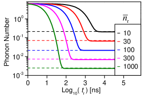
Figure 4: Mean phonon number in the resonator mode $\langle\hat{b}^{{\dagger}}\hat{b}\rangle$ as a function of time starting from an initial occupancy $\bar{n}_{0}=\bar{n}_{\text{th}}=6.4$ (corresponding the parameters in the main text, $T_{\text{bath}}=1.6$ K and $\Omega_{m}=5.1$ GHz) for increasing cooling laser power, expressed as intracavity photon number $N_{\text{r}}$ at the lower sideband frequency. Solid lines: calculations from the Langevin equations neglecting counter-rotating terms, i.e. without quantum backaction (see section I). Dashed lines: expected final occupancy in the resolved sideband regime when accounting for quantum backaction. For this range of cooling powers quantum backaction effects are negligible.

In the main text we consider that the mechanical oscillator is optically cooled to an initial occupancy $\bar{n}_{0}=10^{-2}$ whereas the bath temperature $T_{\text{bath}}=1.6$ K corresponds to an average phonon number $\bar{n}_{\text{th}}=6.4$ at 5.1 GHz. Here we justify the feasibility of this scenario and show that re-cooling can be achieved within $\sim 100$ ns after each write/readout sequence, setting an upper bound of 10 MHz to the repetition rate of the experiment. In Fig. 4 we show the time evolution of the phonon population $\langle\hat{b}^{{\dagger}}\hat{b}\rangle$ calculated from the linearized Langevin equations (scetion I). When the oscillator is initially in equilibrium with the bath, we find that a final occupancy below $10^{-2}$ can be reached for $\bar{n}_{\text{r}}\gtrsim 300$, which is still well in the weak-coupling regime. Since in our calculations we neglect the counter-rotating terms at $\pm 2\Omega_{m}$ there is no limiting quantum backaction. To check that this effect is negligible, we also plot in Fig. 4 the formula derived elsewhere Liu et al. (2013) (under the resolved-sideband approximation)

$$\langle\hat{b}^{{\dagger}}\hat{b}\rangle_{\text{fin}}=\frac{\gamma(4g_{0}^{2}\bar{n}_{\text{r}}+\kappa^{2})}{4g_{0}^{2}\bar{n}_{\text{r}}(\kappa+\gamma)}\bar{n}_{\text{th}}+\frac{\kappa^{2}+8g_{0}^{2}\bar{n}_{\text{r}}}{16(\Omega_{m}^{2}-4g_{0}^{2}\bar{n}_{\text{r}})}$$ (30)

where the second term accounts for the quantum backaction limit to cooling. It can be seen that the deviation due to quantum backaction is indeed very small even for $\bar{n}_{\text{r}}=1000$. Since $\bar{n}_{\text{r}}=|\frac{-is_{-}}{i\Omega_{m}+\kappa/2}|^{2}=\frac{\kappa P_{-}}{\hbar\omega_{c}(\Omega_{m}^{2}+\kappa^{2}/4)}$ this value of $\bar{n}_{\text{r}}$ corresponds to 150 $\mu$W of external laser power, which emphasizes the need for good thermalization of the device in the cryostat to avoid heating the bath due to spurious light absorption.