Abstract

The spatiotemporal complexity induced by perturbed initial excitations through the development of modulational instability in nonlinear lattices with or without disorder, may lead to the formation of very high amplitude, localized transient structures that can be named as extreme events. We analyze the statistics of the appearance of these collective events in two different universal lattice models; a one-dimensional nonlinear model that interpolates between the intergable Ablowitz-Ladik (AL) equation and the nonintegrable discrete nonlinear Schrödinger (DNLS) equation, and a two-dimensional disordered DNLS equation. In both cases, extreme events arise in the form of discrete rogue waves as a result of nonlinear interaction and rapid coalescence between mobile discrete breathers. In the former model, we find power-law dependence of the wave amplitude distribution and significant probability for the appearance of extreme events close to the integrable limit. In the latter model, more importantly, we find a transition in the the return time probability of extreme events from exponential to power-law regime. Weak nonlinearity and moderate levels of disorder, corresponding to weak chaos regime, favor the appearance of extreme events in that case.

Chapter 0 Extreme Events in Nonlinear Lattices

1 Introduction

The inspiring work of John S. Nicolis on hierarchical systems has shown the significance and role of the linkage of different scales [1]. Rogue waves may be seen as a form of an extreme yet emergent property of a complex system attributed to multiple scale hierarchies. Rogue or freak waves are isolated, gigantic water waves that have been observed to appear suddenly in relatively calm seas and disappear without a trace [2]. Although rare, the probability of appearance of these extreme events (EE), loosely defined as highly intense, spatially localized and temporally transient structures [3], seems to be much higher than that expected from normal, Gaussian statistics. Their theoretical analysis has been traditionally linked to nonlinearities and/or randomness in the water wave equations [4, 5, 6, 7, 8, 9]. Recently, super rogue waves have been observed in a water-wave tank due to nonlinear focusing of the local wave amplitude [10]. The occurrence of EEs is not however limited to water waves; in physics, in particular, EEs have been observed in a variety of systems, ranging from optical fibers [11, 12, 13, 14], nonlinear optical cavities [15], superfluid ₄He [16], and laser pulse filamentation [17, 18], to capillary waves [19], space plasmas [20], optically injected semiconductor laser [21], and mode-locked fiber lasers operating in a strongly dissipative regime [22]. The existence of EEs has also been predicted for Bose-Einstein condensates [23], arrays of optical waveguides [24], and soft glass photonic crystal fibers [25].

In nonlinear systems, EEs may appear because of the development of Benjamin-Feir (modulational) instability (MI) for certain types of nonlinearity [26]. The theoretical investigations on EEs follow different paths; one approach adopts the nonlinear Schrödinger (NLS) equation as a universal model and emphasize the mechanisms generating short-lived soliton-like modes [6, 27, 8, 9, 28, 29]. In this approach EEs are singular events localized in space that may be solutions of NLS-type equations with low-order (viz. cubic) nonlinearities. For example, excitations in the form of Akhmediev breathers [30, 31, 32] and Peregrine solitons [33] may be formed and coalesce, resulting in the generation of EEs. Other approaches, following techniques and concepts of hydrodynamics, go beyond the cubic nonlinearity in an attempt to retain some of its complexity [34, 35, 36] and focus primarily on waves in continuous media; however, a wide class of interesting problems involves wave propagation in discrete periodic media forming lattices [37]. Notably, MI may also develop in nonlinear lattices [38], and then discrete NLS (DNLS) models are relevant to the wave propagation in such systems as, e.g., in nonlinear waveguide arrays. It should be noted here that nonlinearity is not a necessary condition for the appearance of EEs; experiments in optics and microwaves indicate that EEs may be triggered in linear systems due to some kind of randomness [39, 14]. A recent review on rogue waves and their generating mechanisms in different physical contexts is given in Ref. [40]. Substantial research efforts have been devoted the last few years to clarify issues related to the probability distributions of EEs, the effect of initial conditions, and the role of nonlinearity and/or disorder. The issue of the interplay between disorder and nonlinearity, often simultaneously encountered in nature and laboratory experiments, and how it affects the probability distribution of EEs, is of particular importance.

Nonlinear lattices form a unique workplace where several processes of different physical nature appear simultaneously and affect their dynamical properties [41]. They constitute prototypical systems of high spatiotemporal complexity that can be investigated theoretically and experimentally, providing a wealth of information on the physics of extended complex systems. The presence of quenched disorder, introduces additionally a mechanism for local symmetry breaking that affects their long-term dynamics [42, 43, 44, 45, 46]. Self-organization is one particular feature of nonlinear lattices that is connected to the possibility for the appearance of EEs. In this aspect, the MI plays an important role as an ”intrinsic noise” in triggering self-organization, as has been indicated by John S. Nicolis and coworkers a long time ago [47]. In this chapter we review some aspects of the role of integrability and the interplay between disorder and nonlinearity in one- and two-dimensional lattices described by discrete nonlinear equations. In the next section, using a one-dimensional discrete nonlinear model that interpolates between the DNLS equation and the Ablowitz-Ladik (AL) equation by varying a single control parameter, we obtain the optimal regime for EE generation and their probability distribution [48]. While the production of EEs in nonlinear systems is mediated by MI, the subsequent evolution reveals complex behavior and their probability of appearance depends on the interplay of nonlinearity and/or disorder, as well as the degree of integrability of the system. We found that integrability properties of the lattice do play a role in the probability of appearance of EEs [48], and that the optimal regime for EE appearance is close to the integrable limit. Importantly, the wave height amplitude distributions match to power-law functions. A broader perspective is obtained in section 3 through a physically realizable model, viz. that of the two-dimensional DNLS equation in the presence of disorder of the Anderson type [49, 50]. In that case, the optimal regime for EE appearance requires weak nonlinearity and moderate levels of disorder [51]. Furthermore, we find a transition in the the return time probability of EEs from exponential to power-law regime, related to a corresponding transition of the system from strong to weak chaos. Thus, the investigation of both models consistently leads to the more general conclusion that the enhancement of probability of appearance of EEs is related to weak chaos, since nearly integrable, modulationally unstable systems may easily fall into a weakly chaotic state.

2 Integrability versus non-integrability

We consider the following model, often referred to as the Salerno model [52]

$$i\frac{d\psi_{n}}{dt}=-(1+\mu|\psi_{n}|^{2})(\psi_{n+1}+\psi_{n-1})-\gamma|\psi_{n}|^{2}\psi_{n}$$ (1)

where $\mu$ and $\gamma$ are two nonlinearity parameters and $n=1,2,3,...,N$. When $\mu=0$ the model becomes the non-integrable DNLS equation while for $\gamma=0$ it reduces to the integrable AL equation. The norm $P_{N}$ and the Hamiltonian $H$ of the model Eq. (1), given respectively by

$$P_{N}=\frac{1}{\mu}\sum_{n}\ln{|1+\mu|\psi_{n}|^{2}|},$$ (2)

and

$$H=\sum_{n}\left[\frac{\gamma}{\mu^{2}}\ln|1+\mu|\psi_{n}|^{2}|-\frac{\gamma}{\mu}|\psi_{n}|^{2}-2Re[\psi_{n}\psi_{n+1}^{*}]\right],$$ (3)

are both conserved quantities. Eq. (1) exhibits MI that may lead to stationary solutions in the form of discrete breathers (DBs)[41], i.e., periodic and spatially localized nonlinear excitations. The DBs thus generated appear in random positions in the lattice and they interact with each other, with the high-amplitude DBs absorbing the low-amplitude ones. After sufficient time, only a small number of high-amplitude DBs that are pinned at particular lattice sites are left, which form virtual bottlenecks that slow down the relaxation processes in the lattice [53, 54]. Transient DBs, however, provide an attractive model of EEs in lattices [31]. The possibility of MI development in Eq. (1) can be investigated within linear stability analysis of its the plane wave solutions modulated by small phase and amplitude perturbations [55]. The relative strength of the on-site and the nonlinear interaction terms, which is affected by the parameters $\mu$ and $\gamma$, may change MI properties and, consequently, the conditions for transient localization. For later convenience, the variables $\psi_{n}$ in Eq. (1) are rescaled according to $\psi_{n}=\xi_{n}/\sqrt{\mu}$, that results in the equation

$$i\frac{d\xi_{n}(t)}{dt}=-(1+|\xi_{n}(t)|^{2})(\xi_{n+1}+\xi_{n-1})-\Gamma|\xi_{n}(t)|^{2}\xi_{n},$$ (4)

where $\Gamma=\gamma/\mu$. Therefore, the whole two-dimensional parameter space $(\gamma,\mu)$ can be scaled by $\mu=1$, that leaves $\gamma$ as a free parameter. With that scaling, the DNLS limit is reached for very large values of $\Gamma$. However, the exact DNLS limit $\mu=0$ has to be calculated separately.

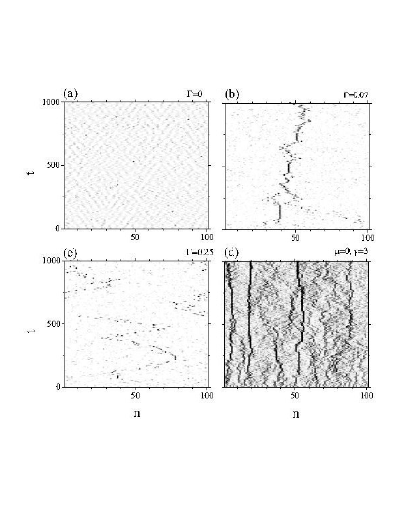
Figure 1: Evolution of the scaled amplitudes $|\xi_{n}|$ for a lattice of size $N=101$, with $\Gamma$ ($\mu$ and $\gamma$ in the DNLS case), is shown on the figure. The initial conditions for all cases are $\xi_{n}=1$ for any $n$ (uniform) plus a small amount of white noise.

Eqs. (4) are integrated with a $6-$th order Runge-Kutta algorithm with fixed time-stepping $\Delta t=10^{-4}$. Periodic boundary conditions are used throughout this section, while the system is initiated with a uniform function $\xi_{n}=1$ for any $n$, which is linearly unstable. A small amount of white noise was added to the initial condition to accelerate the development of MI. Different choices of initial conditions give similar results. Variation of the parameter $\Gamma$ reveals three different regimes illustrated in the spatiotemporal patterns shown in Fig. 1.

(i) For the completely integrable AL lattice ($\Gamma=0$), DBs are mobile and essentially noninteracting; as a result, the formation of EEs in this regime is insignificant (Fig. 1a).

(ii) In the vicinity of the AL limit, i.e. for small values of $\Gamma$ ($\sim 0.1$), the onset of weak interaction between localized modes that can be observed leads to a significant increase of EE formation (Figs. 1b,c). In this regime the mobility of DB excitations is rather high, indicating that DB merging could be responsible for the appearance of EEs.

(iii) For $\Gamma>>0.1$, the dominant behavior is of the DNLS-type, exhibiting localized structures generated through MI that are subsequently pinned at particular lattice sites (Fig. 1d).

[ The height probability density $P_{h}(h)$ for several values of $\Gamma$. The dotted curve corresponds to the DNLS limit (with $\gamma=6$). ] [ The normalized probability for the appearance of extreme events $P_{ee}$ as a function of the integrability parameter $\Gamma$. ]

The calculated height probability distributions (HPD) $P_{h}(h)$ shown in Fig. 2 are in accordance with the earlier observations. The forward (backward) height $h$ at the $n-$th site is defined as the difference between two successive minimum (maximum) and maximum (minimum) values of $|\xi_{n}(t)|$. Both the forward and backward heights are then used for the calculation of the local height distribution; the HPDs are eventually obtained by spatial averaging of all local height distributions. The tails of the HPDs shown in the figure for finite $\Gamma$ are rather long, while in some cases they form a plateau, indicating that EEs with height several times that of the mean of the distribution are probable to appear. In the DNLS limit ($\Gamma\gg 1$), the HPDs are very close to a Rayleigh distribution which tails decay exponentially [56], indicating negligible probability for the appearance of EEs (dotted curve in Fig. 2).

In order to calculate the probability of appearance of EEs, we adopt the criterion employed frequently in the context of water waves and define as an EE a wave which height is greater than $h_{th}$, where $h_{th}=2.2h_{s}$, with $h_{s}$ being the significant wave height. The latter is defined as the average height of the one-third higher amplitude waves in the height distribution. The probability for the appearance of EEs $P_{ee}=P_{h}(h>h_{th})$ is then obtained by integration of the corresponding (normalized) HPD from $h=h_{th}$ up to infinity. Following this procedure, the probability of EE appearance, $P_{ee}$, is calculated as a function of $\Gamma$ (Fig. 2). As can be observed in this figure, $P_{ee}$ has a finite value in the integrable AL case ($\Gamma=0$) around $0.2$. Then, it increases with increasing $\Gamma$ and forms a resonance-like peak with maximum at $\Gamma\simeq 0.07$. Further increase of $\Gamma$ leads to a decrease of $P_{ee}$, that becomes vanishingly small for $\Gamma>>1$. This behavior is compatible with the DB picture outlined earlier, which indicates that the weakly nonlinear, nearly integrable regime is favorable for the appearance of EEs.

3 The two-dimensional DNLS model

We consider the dynamics in a two-dimensional tetragonal lattice with diagonal disorder, or, equivalently, wave propagation in a two-dimensional array of evanescently coupled optical nonlinear fibers with random index variation, both described through the disordered DNLS equation, viz.

$$i\frac{d{\psi}_{n,m}}{dt}={\epsilon}_{n,m}{\psi}_{n,m}+J({\psi}_{n+1,m}+{\psi}_{n-1,m}+{\psi}_{n,m+1}+{\psi}_{n,m-1})+\gamma\left|{\psi}_{n,m}\right|^{2}{\psi}_{n,m},$$ (5)

where $n,m=1,...,N$, $\psi_{n,m}$ is a probability (or wave) amplitude at site $(n,m)$ , $J>0$ is the inter-site coupling constant accounting for tunnelling between adjacent sites of the lattice (corr. evanescent coupling), $\gamma$ is the nonlinearity parameter that stems from strong electron-phonon coupling (corr. Kerr nonlinearity), while ${\epsilon}_{n,m}$, is the local site energy (related to the fiber refractive index), chosen randomly from a uniform, zero-mean distribution in the interval $[-W/2,+W/2]$. Equation (5) serves as a paradigmatic model for a wide class of physical problems where both disorder and nonlinearity are present. For $\gamma\rightarrow 0$, Eq.(5) reduces to the 2D Anderson model while in the absence of disorder (${\epsilon}_{n,m}=0$), it reduces to the DNLS equation in two dimensions that is generally non-integrable. Eq. (5) conserves the norm

$$P_{N}=\sum_{n=1}^{N}\sum_{m=1}^{M}|{\psi}_{n,m}|^{2},`$$ (6)

and the Hamiltonian $\cal{H}$, corresponding to total probability (corr. input power) and the energy of the system, respectively. In optics, the sign of the nonlinearity strength $\gamma$ determines the focussing ($\gamma>0$) or defocusing ($\gamma<0$) properties of the nonlinear medium.

Eqs. (5), implemented with periodic boundary conditions, are integrated using a $6-$th order Runge-Kutta solver with fixed time-stepping [48], for several values of $W$ and $\gamma$ ($J=1$), for a lattice with $N=41$. Larger lattices (i.e., with $N=81$) give similar results. The system is initialized with a uniform state that is slightly modulated by periodic perturbations in order to facilitate the development of MI [38, 57]. The MI threshold for Eq. (5) in the absence of disorder can be obtained using the standard linear analysis, as in the previous section. The MI induces nonlinearly localized modes that are, however, modified by the presence of the quenched disorder. In the time scale of the numerical study, the presence of disorder induces additional energy redistribution among the lattice sites. Thus, it weakens the energy self-trapping which in two dimensions would result in strongly pinned and highly localized breathers [58].

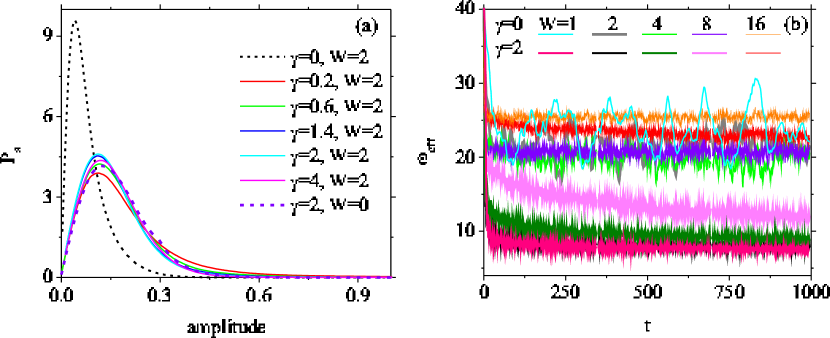
Figure 2: (color online) (a) Amplitude probability distributions as a function of amplitude $P_{s}(|\psi|)$ for several nonlinearity strengths and $W=2$. (b) Effective localization length $w_{eff}$ of the localized structures formed in the lattice as a function of time $t$ for several levels of disorder and $\gamma=0,~{}2$.

The criterion for defining an EE is the same as in the previous section, with the obvious replacement of $|\xi_{n}(t)|$ by $|\psi_{n,m}(t)|$ in the definition of the wave height $h$. During relatively long time (typically $\sim 10^{3}$ time units or equivalently approximately $500$ coupling lengths) the system self-organizes and localized structures appear on different sites that are surrounded by irregular, low-amplitude background. Some of these structures are in the form of DBs, either pinned or mobile, while some others are transient. The complete amplitude statistics for the observed time interval is shown in Fig. 2a for several levels of disorder $W$ and focusing nonlinearity strengths $\gamma$; In all cases, we observe Rayleigh-like distributions which parameters depend on $\gamma$ and $W$. Any state of the lattice that appears with probability in the long tails of these distributions is a potential candidate for an EE. In order to quantify the onset of EEs in the lattice, several statistical measures have been used, viz. the probability for the appearance of EEs, $P_{ee}$, the first appearance and recurrence EE times, $R$ and $P_{r}$, respectively, as well as the inverse participation ratio

$$P={P_{N}^{2}}\left\{\sum_{n=1}^{N}\sum_{m=1}^{M}|f_{n,m}|^{4}\right\}^{-1},$$ (7)

where $P_{N}$ is the norm. We may then define the effective localization length

$$w_{eff}=P^{1/2},$$ (8)

which provides the average spatial extent of the structures formed after the development of MI (Fig. 2b). Note that increasing strength of focusing nonlinearity ($\gamma>0$) decreases $\omega_{eff}$ (enhances localization), while increasing the magnitude of the defocusing nonlinearity increases $\omega_{eff}$ (reduces localization).

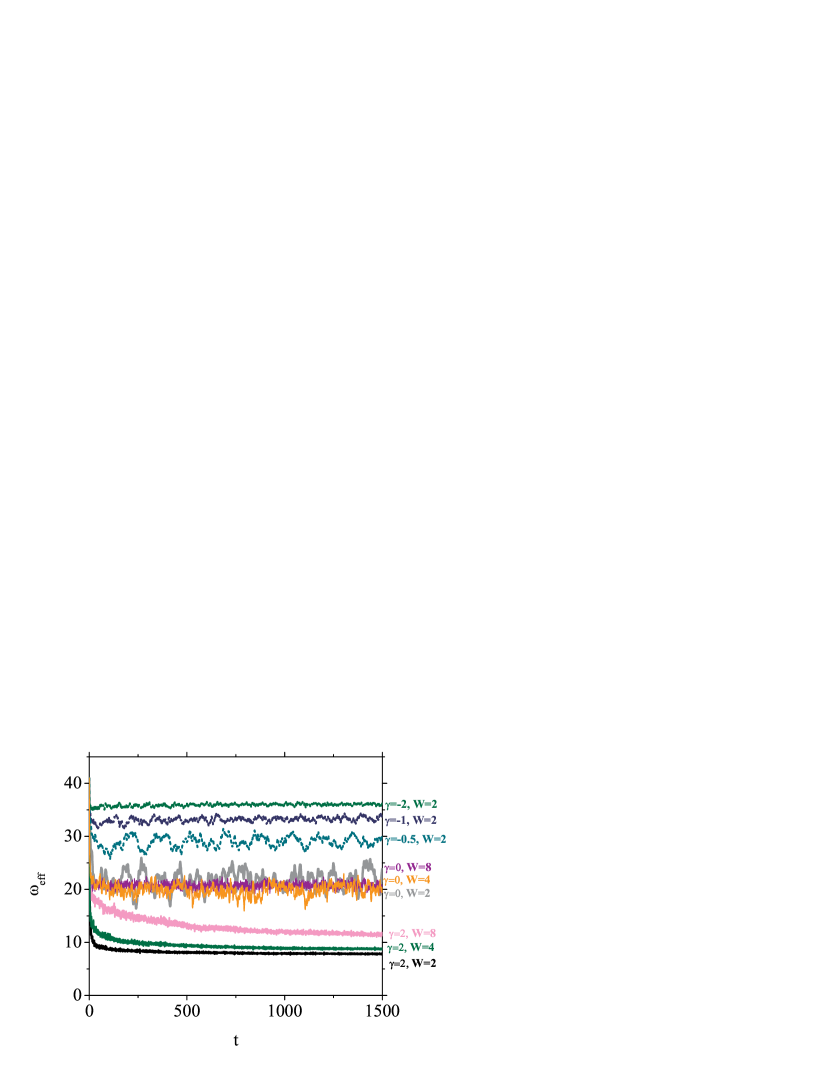
Figure 3: (color online) Comparison of the effective averaged localization length $\omega_{eff}$ as a function of time $t$ for several levels of disorder and both focusing and defocusing nonlinearities.

Both disorder and nonlinearity, each acting alone, favor wave localization in the lattice. When they are simultaneously present, quenched disorder dominates the early stage dynamics since MI develops slowly, at least for relatively small nonlinearity strengths. In this regime, Anderson-like localized states decay spatially while still permitting local energy redistribution until a lower-energy stable localized state is reached. As it can be observed in Fig. 2b, in the presence of nonlinearity, the effective localization length $w_{eff}$ saturates to a value lower than that for the corresponding linear lattice for a wide range of disorder levels. This tendency is compatible with the findings in Ref. [49], where it was also observed that increasing self-focusing strength enhances localization. On the other hand, $w_{eff}$ increases with increasing level of disorder, favoring de-localization. The tendency of disorder-induced-delocalization in the presence of nonlinearity can be attributed to the partial destruction of pinned, highly localized DBs for relatively high levels of disorder. In the case of defocusing nonlinearity (Fig 3), $w_{eff}$ increases with increasing magnitude of the nonlinearity strength.

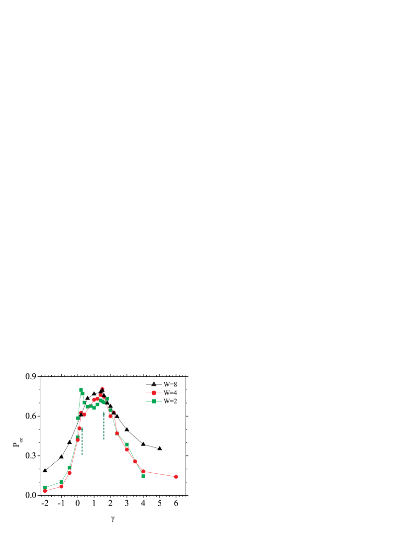
Figure 4: (color online) Extreme event height probability $P_{ee}$ as a function of the nonlinearity strength $\gamma$ for several levels of disorder $W$.

For obtaining the favorite parameter intervals for the appearance of EEs, we calculate numerically $P_{ee}$ as in the previous section as a function of $\gamma$ for three levels of disorder (Fig. 4). Note that both negative and positive values of $\gamma$ have been included in this figure. Referring to the case of high disorder level, we observe that the probability $P_{ee}$ increases with $\gamma$ increasing from negative values, until it reaches a maximum that is located at small positive $\gamma$. Further increase of $\gamma$ decreases $P_{ee}$. For lower levels of disorder, the calculated $P_{ee}(\gamma)$ dependencies exhibit secondary maxima. Also, the decrease of $P_{ee}(\gamma)$, for $\gamma$ moving away from its values at the maxima on either side, is much faster compared to that for high levels of disorder. For zero nonlinearity $P_{ee}$ has still appreciable values; we obtain $P_{ee}=0.47,~{}0.44$ for disorder levels with $W=2,~{}4$, respectively. Thus, according to Fig. 4, the appearance of EEs is favored in the part of parameter space that corresponds to weak nonlinearity strengths $\gamma$ and moderate levels of disorder $W$. For lower levels of disorder ($W=2,4$), the first local maximum can be correlated with the high $P_{ee}$ for the nearly integrable lattice discussed in the previous section [48]. On the other hand, for arbitrary level of disorder, the self-trapping effect of nonlinearity seems to be responsible for the appearance of the second local maximum at $\gamma\approx 2$ with $P_{ee}\approx 0.7\%$.

For gaining deeper understanding of the appearance of EEs in disordered nonlinear lattices, we calculate the return time probabilities $P_{r}$ as a function of the recurrence time $r$ of EEs, and the mean recurrence time $R$ of an EE as a function of the wave height threshold $q$ [59, 60], for focusing nonlinearity. The slope of $R$ as a function of $q$ is smaller in a linear disordered lattice compared to that of a nonlinear disordered lattice for any level of disorder [51]. Also, $R$ increases with increasing $q$ for any $W$ and $\gamma$; that increase is however faster for lower disorder level and stronger nonlinearity. The regime of strong nonlinearity and low level of disorder favors the creation of highly pinned, immobile DBs through self-trapping, increasing thus dramatically the mean recurrence time $R$. The return time probabilities $P_{r}$ are calculated for several values of $W$ and $\gamma$, and shown in Fig. 5. For a given threshold $q$ ($q>h_{th}$) we scan the lattice to find an event at a given location with amplitude larger than $q$. We then register as recurrence time $r$, the time interval between this event and a subsequent one with amplitude larger than $q$ that appears at the same location. We follow this procedure repeatedly up to maximum time and construct distributions that are scaled by the average return time $R\equiv R(q)$, like those shown in Fig. 5. For linear lattices in the presence of disorder, $P_{r}$ as a function of $r/R$ fits to a power-law function of the form

$$P_{r}=\left[a+b\left(\frac{r}{R}\right)\right]^{(-1/c)},$$ (9)

with $1/c$ being  $1.34$ and  $2.46$ for $q=0.66$ and $q=0.33$, respectively. Generally speaking, the presence of nonlinearity reduces the probability of EE appearance. Remarkably, the $P_{r}$ vs. $r/R$ curves in Fig. 5 (a) make a transition from a power-law, in the linear disordered regime, to a double exponential for intermediate nonlinearity, to a single exponential in the nonlinear ordered regime. This transition is linked to the behavior of the tail of the corresponding amplitude probability distributions. In addition we found that the exponential decay of the curves is faster for higher nonlinearity strength. Note that these observations are in accordance to the return time distribution transition from power-law to exponentially like one with increasing nonlinearity parameter in the 1D lattice model presented in previous section (see Fig. 5 (b)).

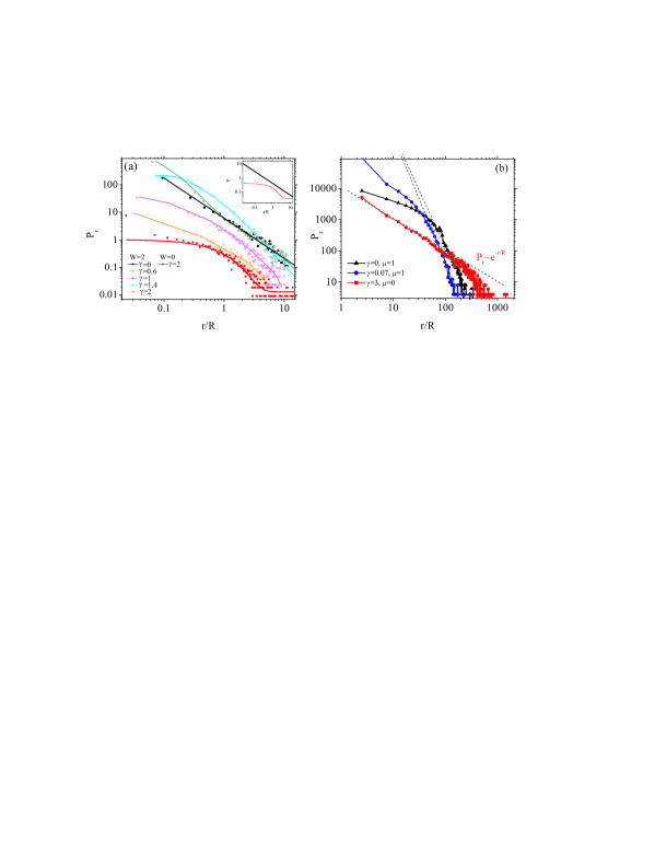
Figure 5: (color online) (a) Return time probability $P_{r}$ (not normalized) as a function of $r/R$ ($q=0.66$), for a linear disordered lattice (power law fit - black curve), a nonlinear ordered (exponential fit - red line) and intermediate cases (double exponential fits). Inset: the first two cases are shown separately. (b) The $P_{r}$ (not normalized) for the Salerno lattice for parameters written in figure.

Recent work on the disordered DNLS equation has proposed a ”phase diagram” that points the different regimes of wave-packet spreading [61, 62]. Our relatively short-time results could be related to expected long-time wave-packet spreading regimes summarized in these references. Different regimes are obtained for

(i) $\delta>2$, onset of self-trapping,

(ii) $d<\delta<2$, strong chaos, and

(iii) $\delta<d$,

where

$$d\approx\frac{\Delta}{V}=\frac{(8J+W)}{w_{eff}},\qquad\delta\approx\gamma,$$ (10)

are the average frequency spacing of the nonlinear modes $\delta$ within a localization volume $V$, and the nonlinear frequency shift, respectively. The selection of the regimes (i)-(iii) was done taking into account the intensity of interaction among the nonlinear modes; the latter increases with the nonlinearity strength up to the high nonlinearity (here $\delta\approx 2$) when the strong self-trapping results in the creation of isolated, strongly pinned, high amplitude DBs. The comparison is only approximate but leads to interesting observations (see Fig. 3). The first local maximum in the $P_{ee}$ for weak nonlinearity is located in the weak chaos regime. Its maximal value $P_{ee}\approx 0.8\%$ is observed for small $W$. The second, broader maximum of $P_{ee}$ for all levels of disorder is located in the strong chaos regime relatively close to the border lines with neighboring regimes. On the other hand, we may associate the power-law decay of $P_{r}$ to the weak chaos regime, and the exponential decay to the self-trapping regime. Therefore, transient EEs are more probable in the regime of weak chaos, while the long-lived EEs (high amplitude, strongly pinned DBs) dominate for strong chaos and self-trapping. This enables us to relate the first local maximum in $P_{ee}$ to the weak interaction of transient EEs induced by disorder while the second, broader maximum, to the appearance of longer-lived DBs resulting from the energy redistribution through the strong interaction between nonlinear modes. In Fig. 3 we show a typical spatiotemporal pattern generated in a nonlinear disordered lattice. Note the presence several EEs, from which we can distinguish at least six with very high amplitude.

[(color online) Different regimes of wave-packet spreading in the effective parameter space $(W,d)$. Lines represent regime boundaries $\delta\approx d$ and $\delta=2$. Empty squares denote parameters for which the $P_{ee}$ maxima are found. Lines with arrows show the direction of increasing $P_{ee}$.] [Spatiotemporal distribution of the lattice energy: disorder and self-focusing nonlinearity are $W=2,\,\gamma=2$ at time $t=1900$.]

4 Conclusions.-

Extreme events or rogue waves nowadays appear in many different physical contexts, and their statistics deviates significantly from the Gaussian behavior that was expected for random waves. Among the many works that have appear the last few years investigating different aspects about EE appearance and the responsible mechanisms, relatively few of them are devoted to discrete systems [48, 63, 64, 51]. In particular, the role of integrability on the probability $P_{ee}$ of appearance of EEs and the wave amplitude distributions have been explored in a model that interpolates between a non-integrable and a completely integrable one. The power-law dependence of the distributions reveals that the probability of EE appearance is much more significant than expected from Gaussian statistics. Moreover, the normalized $P_{ee}$ exhibits a resonance-like maximum in the near-integrable limit. These results can be further analyzed with the help of a nonlinear map [48], where the onset of interaction between DBs manifests itself as a transition from local to global stochasticity monitored through the positive Lyapunov exponent.

In the presence of both disorder and nonlinearity there are two processes that now act simultaneously; Anderson localization [65] and self-focusing due to the MI of the CW background. When each of these processes proceeds alone, it favors the formation of localized structures that eventually get pinned in the lattice. When they act simultaneously, however, the system exhibits higher complexity. In the first stages of the evolution, disorder dominates the dynamics; at later stages, however, nonlinearity takes over through the development of MI that activates self-trapping mechanisms and tends to generate pinned, high-amplitude localized structures which inhibit energy exchange between lattice sites. For weak nonlinearity, however, the pinning mechanism is not very effective, facilitating energy exchange between sites and the appearance of high-amplitude, localized, short-lived structures (EEs) at random locations. For moderate levels of disorder, the probability of EE appearance is maximized, giving the resonance-like peaks shown in Fig. 4. The two peaks that are observed for weak nonlinearity, are related to the weak and strong chaos regime. According to previous analysis, the first local maximum in $P_{ee}$ can be related to transient EEs (weak chaos regime), while the second one to the formation of long-lived DBs. The passage from strong to weak chaos, as well as from non-integrability to integrability, is also related to the observed transition in $P_{r}$ vs. $r/R$ from an exponential to a power-law.

5 Acknowledgments

This research was partially supported by the European Union’s Seventh Framework Programme (FP7-REGPOT-2012-2013-1) under grant agreement n^o 316165, and by the Thales Project MACOMSYS, cofinanced by the European Union (European Social Fund - ESF) and Greek National Funds through the Operational Program ”Education and Lifelong Learning” of the National Strategic Reference Framework (NSRF) Research Funding Program: THALES. ”Investing in knowledge society through the European Social Fund”. A. M. and Lj. H. acknowledge support from the Ministry of Education, Science and Technical Development of Republic of Serbia (Project III 45010).

References

- 1. J. S. Nicolis, Dynamics of hierarchical systems: an evolutionary approach. Springer-Verlag, Berlin, Heidelberg (1986).
- 2. N. Akhmediev, A. Ankiewicz, and M. Taki, Waves that appear from nowhere and disappear without a trace, Phys. Lett. A. 373, 675 (2009).
- 3. S. Albeverio, V. Jentsch, and H. K. (Eds.), Extreme events in nature and society. Springer-Verlag, Berlin (2006).
- 4. E. Pelinovsky, T. Talipova, and C. Kharif, Nonlinear dispersive mechanism of the freak wave formation in shallow water, Physica D. 147 (1-2), 83–94 (2000).
- 5. C. Kharif and E. Pelinovsky, Physical mechanisms of the rogue wave phenomenon, Eur. J. Mech. B/Fluids. 22, 603–634 (2003).
- 6. P. K. Shukla, I. Kourakis, B. Eliasson, M. Marklund, and L. Stenflo, Instability and evolution of nonlinearly interacting water waves, Phys. Rev. Lett. 97, 094501 (2006).
- 7. V. P. Ruban, Nonlinear stage of the Benjamin-Feir instability: Three dimensional coherent structures and rogue waves, Phys. Rev. Lett. 99, 044502 (2007).
- 8. B. Eliasson and P. K. Shukla, Numerical investigation of the instability and nonlinear evolution of narrow-band directional ocean waves, Phys. Rev. Lett. 105, 014501 (2010).
- 9. M. Onorato, D. Proment, and A. Toffoli, Triggering rogue waves in opposing currents, Phys. Rev. Lett. 107, 184502 [5 pages] (2011).
- 10. A. Chabchoub, N. Hoffmann, M. Onorato, and N. Akhmediev, Super rogue waves: Observation of a higher-order breather in water waves, Phys. Rev. X. 2, 011015 (2012).
- 11. D. R. Solli, C. Ropers, P. Koonath, and B. Jalali, Optical rogue waves, Nature. 450, 1054 (2007).
- 12. K. Hammani, C. Finot, J. M. Dudley, and G. Millot, Optical rogue-wave-like extreme value fluctuations in fiber raman amplifiers, Opt. Express. 16, 16467 (2008).
- 13. A. Aalto, G. Genty, and J. Toivonen, Extreme-value statistics in suprercontinuum generation by cascaded stimulated raman scattering, Opt. Express. 18, 1234 (2010).
- 14. F. T. Arecchi, U. Bortolozzo, A. Montina, and S. Residori, Granularity and inhomogeneity are the joint generators of optical rogue waves, Phys. Rev. Lett. 106, 153901 (2011).
- 15. A. Montina, U. Bortolozzo, S. Residori, and F. T. Arecchi, Non-gaussian statistics and extreme waves in a nonlinear optical cavity, Phys. Rev. Lett. 103, 173901 (2009).
- 16. A. N. Ganshin, V. B. Efimov, G. V. Kolmakov, L. P. Mezhov-Deglin, and P. V. E. McClintock, Energy cascades and rogue waves in superfluid 4he, J. Phys.: Conf. Series. 150, 032056 (2009).
- 17. J. Kasparian, P. Béjot, J.-P. Wolf, and J. M. Dudley, Optical rogue wave statistics in laser filamentation, Opt. Express. 17 (14), 12070 (2009).
- 18. D. Majus, V. Junka, G. Valiulis, D. Faccio, and A. Dubietis, Spatiotemporal rogue events in femtosecond filamentation, Phys. Rev. A. 83, 025802 (2011).
- 19. M. Shats, H. Punzmann, and H. Xia, Capillary rogue waves, Phys. Rev. Lett. 104, 104503 (2010).
- 20. M. S. Ruderman, Freak waves in laboratory and space plasmas, Eur. Phys. J. Special Topics. 185, 57– (2010).
- 21. C. Bonatto, M. Feyereisen, S. Barland, M. Giudici, C. M. J. R. R. Leite, and J. R. Tredicce, Deterministic optical rogue waves, Phys. Rev. Lett. 107, 053901 (2011).
- 22. C. Lecaplain, P. Grelu, J. M. Soto-Crespo, and N. Akhmediev, Dissipative rogue waves generated by chaotic pulse bunching in a mode-locked laser, Phys. Rev. Lett. 108, 233901 (2012).
- 23. Y. V. Bludov, V. V. Konotop, and N. Akhmediev, Matter rogue waves, Phys. Rev. A. 80, 033610 (2009).
- 24. Y. V. Bludov, V. V. Konotop, and N. Akhmediev, Rogue waves as spatial energy concentrators in arrays of nonlinear waveguides, Opt. Lett. 34, 3015–3018 (2009).
- 25. D. Buccoliero, H. Steffensen, H. Ebendorff-Heidepriem, T. M. Monro, and O. Bang, Midinfrared optical rogue waves in soft glass photonic crystal fiber, Opt. Express. 19, 17973 (2011).
- 26. B. S. White and B. Forneberg, On the chance of freak waves at sea, J. Fluid Mech. 355, 113–138 (1998).
- 27. A. R. Osborne, Nonlinear Ocean Waves and the Inverse Scattering Transform. Elsevier, Amsterdam (2010).
- 28. F. Baronio, A. Degasperis, M. Conforti, and S. Wabnitz, Solutions of the vector nonlinear schrödinger equations: Evidence for deterministic rogue waves, Phys. Rev. Lett. 109, 044102 (2012).
- 29. V. E. Zakharov and A. A. Gelash, Nonlinear stage of modulation instability, Phys. Rev. Lett. 111, 054101 [5 pages] (2013).
- 30. N. Akhmediev and V. I. Korneev, Modulation instability and periodic solutions of the nonlinear Schrödinger equation, Theor. Math. Phys. 69, 1089 (1986).
- 31. K. B. Dysthe and K. Trulsen, Note on breather type solutions of the NLS as models for freak-waves, Physica Scripta. T82, 48– (1999).
- 32. V. V. Voronovich, V. I. Shrira, and G. Thomas, Can bottom friction suppress ’freak wave’ formation?, J. Fluid Mech. 604, 263–296 (2008).
- 33. K. L. Henderson, D. H. Peregrine, and J. W. Dold, Rogue waves in oceans, Wave Motion. 29, 341– (1999).
- 34. V. E. Zakharov and A. Dyachenko, About shape of giant breather, Europ. J. Mech. B/Fluids. 29(2), 127–131 (2010).
- 35. V. E. Zakharov and R. V. Shamin, Statistics of killer-waves in numerical experiments, JETP Lett. 96(1), 68–71 (2012).
- 36. U. Bandelow and N. Akhmediev, Persistence of rogue waves in extended nonlinear Schrödinger equation, Phys. Lett. A. 376, 1558–1561 (2012).
- 37. D. Hennig and G. P. Tsironis, Wave transmission in nonlinear lattices, Phys. Rep. 307 (5-6), 333–432 (1999).
- 38. Y. S. Kivshar and M. Salerno, Modulational instabilities in the discrete deformable nonlinear Schrödinger equation, Phys. Rev. E. 49, 3543– (1994).
- 39. R. Höhman, U. Kuhl, H.-J. Stöckmann, L. Kaplan, and E. J. Heller, Freak waves in the linear regime: A microwave study, Phys. Rev. Lett. 104, 093901 (2010).
- 40. M. Onorato, S. Residori, U. Bortolozzo, A. Montina, and F. Arecchi, Rogue waves and their generating mechanisms in different physical contexts, Phys. Rep. 528 (2), 47–89 (2013).
- 41. S. Flach and A. V. Gorbach, Discrete breathers - advances in theory and applications, Phys. Rep. 467, 1–116 (2008).
- 42. M. I. Molina and G. P. Tsironis, Absence of localization in a nonlinear random binary alloy, Phys. Rev. Lett. 73, 464–467 (1994).
- 43. G. Kopidakis and S. Aubry, Discrete breathers and delocalization in nonlinear disordered systems, Phys. Rev. Lett. 84 (15), 3236–3239 (2000).
- 44. G. Kopidakis, S. Komineas, S. Flach, and S. Aubry, Absence of wave packet diffusion in disordered nonlinear systems, Phys. Rev. Lett. 100, 084103 (2008).
- 45. S. Flach, D. Krimer, and C. Skokos, Universal spreading of wave packets in disordered nonlinear systems, Phys. Rev. Lett. 102, 024101 [4 pages] (2009).
- 46. A. S. Pikovsky and D. L. Shepelyansky, Destruction of Anderson localization by a weak nonlinearity, Phys. Rev. Lett. 100, 094101 (2008).
- 47. J. S. Nicolis, E. N. Protonotarios, and E. Lianos, Some views on the role of noise in ’self-organizing’ systems, Biol. Cybernetics. 17, 183–193 (1975).
- 48. A. Maluckov, L. Hadžievski, N. Lazarides, and G. P. Tsironis, Extreme events in discrete nonlinear lattices, Phys. Rev. E. 79 (2), 025601(R) [4 pages] (2009).
- 49. T. Schwartz, G. Bartal, S. Fishman, and M. Segev, Transport and Anderson localization in disordered two-dimensional photonic lattices, Nature. 446, 52–55 (2007).
- 50. Y. Lahini, A. Avidan, F. Pozzi, M. Sorel, D. N. C. R. Morandotti and, and Y. Silberberg, Anderson localization and nonlinearity in one-dimensional disordered photonic lattices, Phys. Rev. Lett. 100, 013906 (2008).
- 51. A. Maluckov, N. Lazarides, G. P. Tsironis, and L. Hadžievski, Extreme events in two-dimensional nonlinear lattices, Physica D. 252, 59–64 (2013).
- 52. M. Salerno, Discrete model for dna-promoter dynamics, Phys. Rev. A. 44, 5292–5297 (2001).
- 53. G. P. Tsironis and S. Aubry, Slow relaxation phenomena induced by breathers in nonlinear lattices, Phys. Rev. Lett. 77, 5225–5228 (1996).
- 54. K. Ø. Rasmussen, S. Aubry, A. R. Bishop, and G. P. Tsironis, Discrete nonlinear Schrödinger breathers in a phonon bath, Eur. Phys. J. B. 15, 169– (2000).
- 55. A. Maluckov, L. Hadžievski, and B. Malomed, Dark solitons in dynamical lattices with the cubic-quintic nonlinearity, Phys. Rev. E. 76, 046605 (2007).
- 56. N. G. Van-Kampen, Stochastic Processes in Physics and Chemistry. North-Holland, Amsterdam (1981).
- 57. A. Wöllert, G. Gligorić, M. M. Skorić, A. Maluckov, N. Raicević, A. Danicić, and L. Hadžievski, Modulation instability of two-dimensional dipolar Bose-Einstein condensate in a deep optical lattice, Acta Phys. Pol. A. 116, 519 (2009).
- 58. M. I. Molina, Self-trapping dynamics in two-dimensional nonlinear lattices, Modern Physics Letters B. 13, 837– (1999).
- 59. E. G. Altmann and H. Kantz, Recurrence time analysis, long-term correlations, and extreme events, Phys. Rev. E. 71, 056106 (2005).
- 60. M. S. Santhanam and H. Kantz, Return interval distribution of extreme events and long-term memory, Phys. Rev. E. 78, 051113 (2008).
- 61. T. V. Laptyeva, J. D. Bodyfelt, D. O. Krimer, C. Skokos, and S. Flach, The crossover from strong to weak chaos for nonlinear waves in disordered systems, Europhys. Lett. 91, 30001 (2010).
- 62. S. Flach, Spreading of waves in nonlinear disordered media, Chemical Physics. 375, 548–556 (2010).
- 63. A. Ankiewicz, N. Akhmediev, and J. M. Soto-Crespo, Discrete rogue waves of the Ablowitz-Ladik and Hirota equations, Phys. Rev. E. 82, 026602 (2010).
- 64. N. Akhmediev and A. Ankiewicz, Modulation instability, Fermi-Pasta-Ulam recurrence, rogue waves, nonlinear phase shift, and exact solutions of the Ablowitz-Ladik equation, Phys. Rev. E. 83, 046603 (2011).
- 65. P. W. Anderson, Absence of diffusion in certain random lattices, Phys. Rep. 109, 1492– (1958).