Coulomb and spin-orbit interactions in random phase approximation calculations

Abstract

We present a fully self-consistent computational framework composed by Hartree-Fock plus random phase approximation where the spin-orbit and Coulomb terms of the interaction are included in both steps of the calculations. We study the effects of these terms of the interaction on the random phase approximation calculations, where they are usually neglected. We carry out our investigation of excited states in spherical nuclei of oxygen, calcium, nickel, zirconium, tin and lead isotope chains. We use finite-range effective nucleon-nucleon interactions of Gogny type. The size of the effects we find is, usually, of few hundreds of keV. There are not simple approximations which can be used to simulate these effects since they strongly depend on all the variables related to the excited states, angular momentum, parity, excitation energy, isoscalar and isovector characters. Even the Slater approximation developed to account for the Coulomb exchange terms in Hartree-Fock is not valid in random phase approximation calculations.

I Introduction

The combination of Hartree-Fock (HF) and random phase approximation (RPA) calculations carried out with a unique effective interaction has been able to provide a good description of known nuclear properties in a wide range of the nuclear chart, from light nuclei around the oxygen region up to very heavy nuclei such as the uranium. This success has induced to believe that this computational scheme could provide good predictions of the properties of exotic nuclei which will be produced in the next few years in radioactive ion beams facilities. This possibility has increased the interest in defining more precisely the details of the self-consistent HF plus RPA (HF+RPA) calculations.

In HF calculations, the presence of the spin-orbit term of the interaction is essential to properly describe the shell structure of the various nuclei, and that of the Coulomb interaction to distinguish between proton and neutron single particle (s.p) properties. These two terms of the effective nucleon-nucleon interaction are usually neglected in RPA calculations, since the evaluation of their contributions, considered small as compared to that of the other terms of the interaction, is computationally quite heavy.

The relatively small size of the effects of Coulomb and spin-orbit terms has been confirmed in recent years by the results of some fully self-consistent HF+RPA calculations. The calculations carried out with zero-range Skyrme forces ter05 ; fra05 ; sil06 ; col07 ; los10 ; col13 indicate that spin-orbit and Coulomb interactions produce effects of a few hundreds of keV.

To the best of our knowledge, fully self-consistent HF+RPA calculations with finite-range interactions have been carried out only by using Gogny interactions. In this type of calculations, the results obtained by Péru et al. per05 show that the spin-orbit term of the interaction plays a remarkable role in the structure of the low-lying quadrupole and octupole states by modifying both excitation energies and transition probabilities. In the same work it has been shown that the Coulomb force in RPA calculations significantly affects the centroid energies of the isovector giant dipole resonances and their energy weighted sum rule values. The study of Ref. per05 has ben conducted by considering the doubly magic nuclei ⁷⁸Ni, ¹⁰⁰Sn, ¹³²Sn, and ²⁰⁸Pb with the D1S^′ parameterization of the Gogny two-body effective interaction.

Recently, we have developed an approach to carry out HF+RPA self-consistent calculations with finite-range interactions don11a . We have used this model to study magnetic and electric nuclear excitations with Gogny interactions, but in these investigations the spin-orbit and Coulomb terms of the interactions were not considered in the RPA calculations.

In the present work, we show the results of a study in which we have evaluated the effects of these terms of the D1M parameterization of the Gogny interaction in fully self-consistent HF+RPA calculations. With respect to the investigation of Ref. per05 , we have considered a different interaction, a wider set of spherical nuclei, and we have focussed our attention mainly to low-lying excited states, rather than to the centroid energies of giant resonance excitations. We have studied the validity of the Slater approximation sla51 in the treatment of the Coulomb exchange RPA terms. We have calculated the effects of the spin-orbit and Coulomb terms on low lying $2^{+}$ and $3^{-}$ multipole excitations and the dependence of these effects in isoscalar (IS) and isovector (IV) excitations in nuclei with the same number of protons and neutrons. We have considered excitations dominated by single particle-hole (p-h) pairs and we have studied the evolution of the effects with different values of the angular momentum of the excitations. Our results confirm that the effects of the spin-orbit and Coulomb terms of the interactions are of a few hundreds of keV.

Our model is presented in Sect. II. Details and basic ingredients of the calculations are presented in Sect. III. In Sect. IV we have discussed the effects of the spin-orbit and Coulomb interactions in a selected set of results and studied the validity of the Slater approximation for the Coulomb exchange term. In Sect. V we summarize the main results of our work and we draw our conclusions.

II The model

The only input required by our self-consistent approach is the effective nucleon-nucleon force. We have considered a general finite-range force which we express as

$$\widehat{V}_{\alpha}(i,j)\,=\,v_{\alpha}(r_{ij})\,O^{\alpha}_{i,j}\,,\,\,\,\alpha=1,2,\ldots,8\,,$$ (1)

where $v_{\alpha}$ are scalar functions of the distance between the two interacting nucleons, and $O^{\alpha}$ indicates the type of operator dependence

$$O^{\alpha}_{i,j} : 1\,,\,\,\mbox{\boldmath$\tau$}(i)\cdot\mbox{\boldmath$\tau$}(j)\,,\,\,\mbox{\boldmath$\sigma$}(i)\cdot\mbox{\boldmath$\sigma$}(j)\,,\,\,\mbox{\boldmath$\sigma$}(i)\cdot\mbox{\boldmath$\sigma$}(j)\,\mbox{\boldmath$\tau$}(i)\cdot\mbox{\boldmath$\tau$}(j)\,,$$ (2)

$$S_{ij}\,,\,\,S_{ij}\,\mbox{\boldmath$\tau$}(i)\cdot\mbox{\boldmath$\tau$}(j)\,,\,\,{\bf L}_{ij}\cdot{\bf S}\,,\,\,{\bf L}_{ij}\cdot{\bf S}\,\mbox{\boldmath$\tau$}(i)\cdot\mbox{\boldmath$\tau$}(j)\,.$$

In the above expression $\sigma$ is the Pauli matrix operator acting on the spin variable and $\tau$ the analogous operator for the isospin. The tensor operator is defined as

$$S_{ij}\,=\,3\,\frac{\mbox{\boldmath$\sigma$}(i)\cdot{\bf r}_{ij}\,\mbox{\boldmath$\sigma$}(j)\cdot{\bf r}_{ij}}{r_{ij}^{2}}\,-\,\mbox{\boldmath$\sigma$}(i)\cdot\mbox{\boldmath$\sigma$}(j)\,,$$ (3)

where

$${\bf r}_{ij}\,=\,{\bf r}_{i}\,-\,{\bf r}_{j}$$ (4)

represents the relative coordinate. In the spin-orbit terms of the force, $\alpha=7,8$, we have indicated with

$${\bf L}_{ij}\,=\,{\bf r}_{ij}\times{\bf p}_{ij}$$ (5)

the relative angular momentum of the two interacting nucleons, where their relative momentum has been defined as

$${\bf p}_{ij}\,=\,\frac{1}{2}({\bf p}_{i}-{\bf p}_{j})\,,$$ (6)

and with

$${\bf S}\,=\,{\bf s}_{i}+{\bf s}_{j}$$ (7)

the total spin of the nucleon pair.

With this type of interactions, we solved the HF equations as indicated in Refs. co98 ; bau99 . From the solution of these equations we obtained a set of s.p. wave functions that have been used to solve the RPA equations. We have considered the RPA equations in their matrix formulation fet71 ; rin80 ; suh07 .

We have evaluated the corresponding matrix elements by expressing the force in configuration space as the Fourier transform of the force given in momentum space

$$v_{\alpha}(r_{ij})=\frac{1}{(2\pi)^{3/2}}\int{\rm d}^{3}q\,\exp\left[i{\bf q}\cdot({\bf r}_{i}-{\bf r}_{j})\right]\,\tilde{v}_{\alpha}(q)\,.$$ (8)

In this way, we could separate the coordinates ${\bf r}_{i}$ and ${\bf r}_{j}$ and carry out the multipole expansion of the two exponentials. A detailed derivation of the matrix element expressions for all the force channels up to $\alpha=6$ can be found in Ref. don08t .

In our previous works don11a , the spin-orbit and Coulomb matrix elements have been neglected in RPA calculations, and we have considered them in HF calculations only. The inclusion of the Coulomb interaction in the RPA calculations

$$v_{\rm C}(r_{ij})\,=\,\frac{e^{2}}{|\boldsymbol{r}_{i}-\boldsymbol{r}_{j}|}$$ (9)

is relatively easy, since the RPA matrix elements are identical to those of the scalar term of the interaction (1) (see Ref. don08t ). Obviously, we have to consider that the interaction is active only between proton p-h pairs.

The evaluation of the spin-orbit matrix elements is more involved. We give in Appendix A some details about it. The general expressions presented in this appendix have been obtained by considering that the scalar functions $v_{\alpha=7,8}$ of Eq. (1) have finite-range. In our calculations we used Gogny interactions that include a spin-orbit potential of contact type, analogous to that adopted in Skyrme-like interactions:

$$F_{ij}^{\rm SO}\,=\,2\,i\,W_{0}\,\left[\overleftarrow{{\bf p}}_{ij}\times\delta(r_{ij})\,\overrightarrow{{\bf p}}_{ij}\right]\cdot\mathbf{S}\,,$$ (10)

where the arrows indicate the side on which the operator ${\bf p}_{ij}$ acts. Taking into account the expression

$$\delta(r_{ij})\,=\,\lim_{\mu\to\infty}\,\frac{\mu^{3}}{\pi^{3/2}}\,\exp\left(-\mu^{2}r_{ij}^{2}\right)\,,$$ (11)

we obtain:

$$F_{ij}^{\rm SO} = 2\,i\,W_{0}\,\lim_{\mu\to\infty}\frac{\mu^{3}}{\pi^{3/2}}\left[\overleftarrow{{\bf p}}_{ij}\times\exp\left(-\mu^{2}r_{ij}^{2}\right)\,\overrightarrow{{\bf p}}_{ij}\right]\cdot\mathbf{S}$$ (12)

$$= -\,4\,W_{0}\,\left[\lim_{\mu\to\infty}\,\frac{\mu^{5}}{\pi^{3/2}}\,\exp\left(-\mu^{2}r_{ij}^{2}\right)\right]\,\mathbf{L}_{ij}\cdot\mathbf{S}\,.$$

By comparing the above expression with the $v_{7}$ term of Eq. (1), we identify

$$v_{7}(r_{ij})\,=\,-\,4\,W_{0}\,\lim_{\mu\to\infty}\,\frac{\mu^{5}}{\pi^{3/2}}\,\exp\left(-\mu^{2}r_{ij}^{2}\right)\,$$ (13)

whose Fourier transform is

$$\tilde{v}_{7}(q)\,=\,\lim_{\mu\to\infty}\,\int{\rm d}^{3}r\,\exp\left[-i{\bf q}\cdot({\bf r}_{i}-{\bf r}_{j})\right]\,v_{7}(r)\,=\,W_{0}\,{\bf q}^{2}\,,$$ (14)

which is the expression used in our RPA calculations.

In the following, we indicate with $\omega_{0}$ the excitation energies obtained without spin-orbit and Coulomb interactions in RPA calculations. In analogy, we call $\omega_{\rm C}$, $\omega_{\rm SO}$, and $\omega_{\rm C+SO}$ the energies obtained when, only the Coulomb, or only the spin-orbit term, or both are included.

III Details of the calculations

The results we present in this article have been obtained by using the D1M parameterization gor09 of the Gogny interaction dec80 . We carried out calculations also with the more traditional D1S force ber91 but, since the results are very similar to those obtained with the D1M interaction, we do not show and discuss them here. The D1M interaction is composed by four finite-range terms, the scalar, isospin, spin and spin-isospin dependent terms, a zero-range density dependent term and, in addition, the Coulomb and a zero-range spin-orbit term.

The first step of our calculations consists in constructing the s.p. basis by solving the HF equations with the complete D1M interaction described above. This is done by imposing bound-state boundary conditions at the edge of the discretization box. The technical details concerning the iterative procedure used to solve the HF equations for a density-dependent finite-range interaction can be found in Refs. co98b ; bau99 . When the stable solution, corresponding to the minimum of the binding energy, is reached, the HF equations are solved again, not only for the states below the Fermi surface, but, by using the local Hartree and the non local Fock-Dirac potentials constructed on these s.p. states, also for those states above it. In this manner we generate a set of discrete bound states also in the positive energy region, which should be characterized by the continuum. The level density in the continuum region is strictly related to the size of the space integration box: the larger is the box the higher is the level density.

We write the RPA secular equations rin80 in matrix form and solve them by diagonalization. The dimensions of the matrix to diagonalize are given by the number of the p-h pairs contributing to the specific excitation. This depends on the number of the s.p. states composing the configuration space. In our approach, the results of the RPA calculations depend on two parameters, the level density, which is related to the size of the integration box, and the maximum s.p. energy. We have chosen the values of these two parameters by controlling that the centroid energies of the giant dipole responses do not change by more than 0.5 MeV when either the box size or the maximum s.p. energies are increased. The most demanding calculations are those we carried out for the ²⁰⁸Pb nucleus. In this nucleus, by using a box radius of 25 fm and an upper limit of s.p. energy of 100 MeV, we diagonalise matrices of dimensions of about 1300 $\times$ 1300.

IV Results

In this section we study the effects of the Coulomb and spin-orbit interactions in RPA calculations. For this study we have considered a set of isotopes representative of various regions of the nuclear chart. For the light nuclei we have chosen the oxygen isotopes ¹⁶O, ²²O, ²⁴O, ²⁸O, for the medium nuclei some calcium, ⁴⁰Ca, ⁴⁸Ca, ⁵²Ca, ⁶⁰Ca, and nickel isotopes, ⁴⁸Ni, ⁵⁶Ni, ⁶⁸Ni, ⁷⁸Ni, for the heavier nuclei some tin isotopes, ¹⁰⁰Sn, ¹¹⁴Sn, ¹¹⁶Sn, ¹³²Sn, and, in addition, the ⁹⁰Zr and ²⁰⁸Pb nuclei. Common feature of all these nuclei is that the s.p. levels below the Fermi surface are fully occupied, and those above it are completely empty. This implies that the nuclei we have considered have spherical shape. In addition, since the energy gap between the last occupied s.p. level and the first empty level is relatively large, the pairing effects are negligible. Our calculations do not consider these effects, even though the Hartree-Fock-Bogoliubov calculations of Ref. hil07 indicate the presence of pairing effects in the ²²O, ⁵²Ca, ⁶⁰Ca, ⁶⁸Ni, ⁹⁰Zr, ¹¹⁴Sn and ¹¹⁶Sn nuclei.

First, we have focussed our attention into low-lying quadrupole and octupole electric excitations, more precisely those $2^{+}$ and $3^{-}$ excitations dominated by p-h pairs where the particle is below the continuum threshold. We found $3^{-}$ states with these characteristics for all the nuclei we have investigated. On the contrary, these type of states are not present in the $2^{+}$ excitations of ¹⁶O, ²⁸O, ⁴⁰Ca, ⁶⁰Ca and ⁴⁸Ni. We have studied the effects of the Coulomb force, and the need of an exact treatment of its exchange matrix elements (Sect. IV.1), and then the effects of the spin-orbit interaction (Sect. IV.2). In section IV.3 we have investigated whether the Coulomb and spin-orbit interactions have different effects on IS and IV excitations in nuclei with $N=Z$. In section IV.4 we have studied the sensitivity to Coulomb and spin-orbit terms of those states dominated by a unique s.p. transition, as a function of the angular momentum of the excitation.

IV.1 Effects of the Coulomb force on quadrupole and octupole electric excitations

The use of a finite-range interaction in a fermionic many-body system requires the evaluation of both direct and exchange matrix elements of the force. The evaluation of these latter ones is numerically much more involved than that of the former ones. For this reason, the exchange matrix elements of the Coulomb interaction are often estimated by using a local density approximation, called Slater approximation sla51 , which reduces their contribution to a correction of the direct matrix elements. The validity of the Slater approximation in HF calculations has been investigated for the zero-range Skyrme force tit74 ; ska01 ; blo11 but also for the finite-range Gogny ang01a interaction.

We study the validity of the Slater approximation in RPA calculations by comparing its results with those obtained by exactly evaluating the Coulomb exchange matrix elements. The expression of the Coulomb exchange contribution to the total HF energy in the Slater approximation is col13

$$E_{\rm C,ex}^{\rm Slater}\,=\,-\frac{3e^{2}}{4}\,\left(\frac{3}{\pi}\right)^{1/3}\,\int{\rm d}^{3}r\,\rho_{p}^{4/3}(r)\,,$$ (15)

where $\rho_{p}$ is the proton density. From the above equation we obtain

$$V_{\rm C,ex}^{\rm Slater}(r_{ij})\,=\,-\frac{e^{2}}{3}\,\left(\frac{3}{\pi}\right)^{1/3}\rho_{p}^{-2/3}(r_{j})\,\delta(r_{ij})\,,$$ (16)

which is the exchange Coulomb potential in the Slater approximation to be used in RPA calculations col13 . Specifically, we added this expression to that of the Coulomb potential (9), and calculated only the direct matrix elements.

To study the effects of the Coulomb interaction on the RPA, we use the same set of s.p. states generated by the HF calculations with the full D1M Gogny interaction, and we compare the results obtained without Coulomb interaction with those obtained by including it in the exact manner and in the Slater approximation. In this study the spin-orbit term of the interaction has not been considered in the RPA calculations.

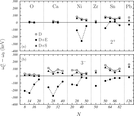
Figure 1: Difference between the RPA energies calculated with and without Coulomb interaction for quadrupole and octupole electric excitations of the nuclei we are investigating. The open squares, $\alpha\equiv$D indicate the results obtained by considering the Coulomb direct term only, the solid circles, $\alpha\equiv$D+E those obtained by considering also the exchange term. The solid triangles, $\alpha\equiv$D+S, show the results obtained by using the Slater approximation to describe the exchange term. All the results of the figure have been obtained without spin-orbit interaction in the RPA calculation. The lines are drawn to guide the eyes.

For the various nuclei we have investigated, we present in Fig. 1 the RPA results for low-lying $2^{+}$ and $3^{-}$ states, panels (a) and (b) respectively, carried out by including the Coulomb interaction. The results presented are the differences between the energies obtained with and without Coulomb interaction, $\omega_{\rm C}^{\alpha}-\omega_{0}$. The open squares, $\alpha\equiv{\rm D}$, indicate the results obtained when only the direct terms of the Coulomb matrix elements are considered, and the solid circles, $\alpha\equiv{\rm D+E}$, when also the exchange matrix elements are included. The solid triangles, $\alpha\equiv{\rm D+S}$, show the results obtained when the Slater approximation of the exchange matrix elements is used.

The results shown in Fig. 1 indicate that the effects of the Coulomb interaction are rather small. We observe maximum differences of the order of few hundreds of keV, in much cases smaller than 100 keV. If only the direct matrix elements are considered the Coulomb interaction is always repulsive: all the nuclei show positive differences, smaller than 100 keV for the $2^{+}$, and smaller than 200 keV for the $3^{-}$. The sign of the difference is reversed when the exchange terms are considered, as the solid circles indicate. The behavior of the complete results strongly depend on the multipolarity and on the nucleus considered. The effects on the $2^{+}$ states of the oxygen and calcium isotopes are negligible, while they become remarkable in the nickel isotopes, more relevant than the effects found in the heavier nuclei we have considered. The situation on the $3^{-}$ states is again different. In this case, the isotopes where we observe the largest effects are those of oxygen and calcium, while the effects on the heavier nuclei become gradually smaller.

The results obtained with the Slater approximation strictly follow those obtained by considering only the direct term, and slightly lower the size of the repulsive effect. The Slater approximation is unable to modify the effects of the direct Coulomb matrix elements to reproduce in a reasonable way the effects of the exchange terms.

IV.2 Effects of the spin-orbit force on quadrupole and octupole electric excitations

We use again the $2^{+}$ and $3^{-}$ states considered in the previous section to discuss the effects of the spin-orbit interaction. The results of the calculations done by including the Coulomb and spin-orbit terms of the interactions for the evaluation of the excitation energy of these multipoles are presented in Fig. 2 as a difference with the energies $\omega_{0}$ obtained without them.

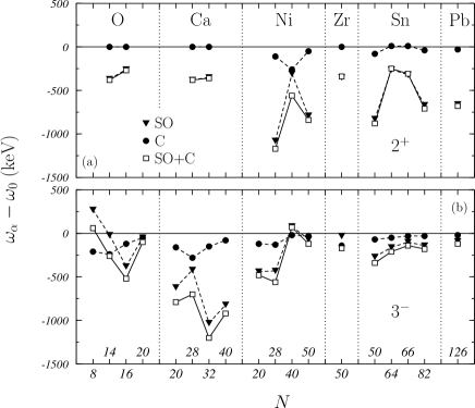
Figure 2: The same as in the previous figure, but now the various symbols represent the RPA energy differences obtained by considering the spin-orbit interaction only (solid triangles), the Coulomb interaction only (solid circles) and both of them (open squares). As in Fig. 1 these results are expressed as differences with the RPA energies calculated without these terms of the interaction. The lines are drawn to guide the eyes.

In Fig. 2 the solid triangles indicate the results obtained by using the spin-orbit force only, while the results of the complete calculations, where both Coulomb and spin-orbit terms are considered, are shown by the open squares. For completeness, we show again, with the solid circles, the results obtained by using the Coulomb interaction only.

We first remark that the effects of the spin-orbit force are, in the great majority of the cases, larger than those of the Coulomb interaction. The second remark is that, in general, the spin-orbit interaction is attractive. The exceptions to this trend that we observe are for the $3^{-}$ excitations of ¹⁶O and of ⁶⁸Ni. The global effect is essentially given by the simple sum of the two effects separately considered. The largest effects are those found for the $3^{-}$ state in ⁵²Ca nucleus and for the $2^{+}$ state in ⁵⁶Ni nucleus where they reach the values of about 1.2 MeV. A comparison of our results with those of Péru et al. per05 for the ⁷⁸Ni, ¹⁰⁰Sn, ¹³²Sn and ²⁰⁸Pb show a good agreement.

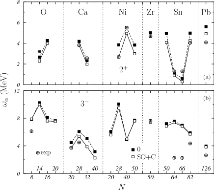
Figure 3: Excitation energies of the lowest collective $2^{+}$ (a) and $3^{-}$ (b) states for the nuclei we are investigating. The solid squares indicate the results obtained by neglecting both Coulomb and spin-orbit interactions and the open squares those obtaind by considering them. These energies are compared with the available experimental values taken from Refs. led78 ; bnlw and represented by the crossed circles. The lines are drawn to guide the eyes.

In Fig. 3 we show the energies of the $2^{+}$ and $3^{-}$ states obtained by using the D1M interaction with and without Coulomb and spin-orbit terms, open and solid squares respectively. We observe that the inclusion of the Coulomb and spin-orbit terms reduces the energy values. We compare the results of our calculations with the available experimental values taken from the compilations of Refs. led78 ; bnlw ; ram01 ; sto05 (crossed circles). The experimental spectrum is much richer than that produced by our calculations, therefore, in some case, the identification of the experimental excited state to be compared with that theoretically found is not free from ambiguities. For this reason, we do not enter in a detailed discussion of each result. In any case, we can state that the comparison shown in Fig. 3 is satisfactory, especially considering that these RPA calculations are parameter free.

The case of the low-lying 2⁺ state in ²⁰⁸Pb has been carefully investigated. Calculations carried out with SLy4 interaction col07 and with the Gogny D1S^′ force per05 indicate that the inclusion of spin-orbit and Coulomb terms reduces the discrepancy between theory and experiment. We observe the same effect also in our calculations, where energy value of 5.61 MeV is reduced to 4.93 MeV when both terms are included. The experimental value is 4.08 MeV (Ref. zie68 ) and the shift of about 0.85 MeV we obtain in our calculation is similar to that found in Refs. per05 ; col07 .

The differences observed for the $3^{-}$ states with respect to the experimental values are smaller than 2 MeV except for ¹¹⁴Sn and ¹¹⁶Sn. In these nuclei, the inclusion of pairing effects improves the agreement ans06 ; car12 .

IV.3 IS and IV excited states

In this section we investigate whether the Coulomb and spin-orbit forces generate different effects on IS and IV excitations. For this study, we have selected cases where the IS and IV characters of the multipole excitation are well identified. We have limited our investigation to nuclei with equal number of protons and neutrons and to multipole excitations dominated by the p-h pairs where particle and hole states are just above and just below the Fermi surface. In this situation, we can identify excited states dominated by the same p-h pairs in both proton and neutron sectors. The quantum numbers identifying the s.p. states of these p-h pairs are the same for protons and neutrons. When the proton and neutron p-h pairs are in phase we have an IS excitation and when they are out of phase we have the IV excitation. Thus, the IS and IV character of the excitation can be easily identified in our RPA calculations by observing the relative sign of the proton and neutron RPA forward $X$ amplitudes defined, as usual rin80 , as

$$|\nu\rangle\,=\,\sum_{ph}\left(X^{\nu}_{ph}\,a^{+}_{p}\,a_{h}\,-\,Y^{\nu}_{ph}\,a^{+}_{h}\,a_{p}\right)|0\rangle\,,$$ (17)

where $|\nu\rangle$ and $|0\rangle$ are the RPA excited and ground states, and $a^{+}$ and $a$ the creation and annihilation s.p. operators.

			excitation energy (MeV)
			IS			IV
nucleus	p-h pair	$J^{\pi}$	$\omega_{0}$	exp		$\omega_{0}$	exp
16O	$1d_{5/2}\,1p_{1/2}^{-1}$	$2^{-}$	9.42	8.87		11.25	12.53
	$1d_{5/2}\,1p_{3/2}^{-1}$	$4^{-}$	16.0	17.79		16.98	18.98
40Ca	$1f_{7/2}\,1d_{3/2}^{-1}$	$2^{-}$	6.51	7.53		8.38	8.42
	$1f_{7/2}\,1d_{3/2}^{-1}$	$4^{-}$	6.66	5.61		7.03	7.66
56Ni	$1f_{5/2}\,1f_{7/2}^{-1}$	$1^{+}$	7.93			11.16
	$2p_{3/2}\,1f_{7/2}^{-1}$	$3^{+}$	5.79			6.21
	$2p_{3/2}\,1f_{7/2}^{-1}$	$5^{+}$	5.99			6.30
100Sn	$1g_{7/2}\,1g_{9/2}^{-1}$	$1^{+}$	7.62			10.37
	$2d_{5/2}\,1g_{9/2}^{-1}$	$3^{+}$	6.53			7.00
	$2d_{5/2}\,1g_{9/2}^{-1}$	$5^{+}$	6.59			6.88

Table 1: Isotopes with equal number of protons and neutrons selected to study the effects of Coulomb and spin-orbit interactions on IS and IV excitations. In the second column we indicate the proton and neutron p-h pairs which dominate the excitations, and in the third column the angular momentum and the parity of the excited states we have considered. The values, in MeV, of the excitation energies $\omega_{0}$, are those obtained without Coulomb and spin-orbit interactions. When available, we present in the columns labelled “exp” the experimental values taken from the compilations of Refs. led78 ; bnlw .

In Table 1 we show the nuclei we have considered, the p-h pairs dominating the transitions, and the angular momentum and parity of the multipole excitation. We also indicate the values of the energies $\omega_{0}$ obtained without the Coulomb and spin-orbit interactions. We compare these energies with the available experimental energies taken from the compilations of Refs. led78 ; bnlw ; ram01 ; sto05 . The information given in Table 1 completes that given in Fig. 4, where the effects of the Coulomb and spin-orbit interaction terms are shown as differences with respect to $\omega_{0}$. The labels C, SO and SO+C indicate the results we have obtained by adding to the D1M interaction only the Coulomb, only the spin-orbit or both terms of the interactions, respectively.

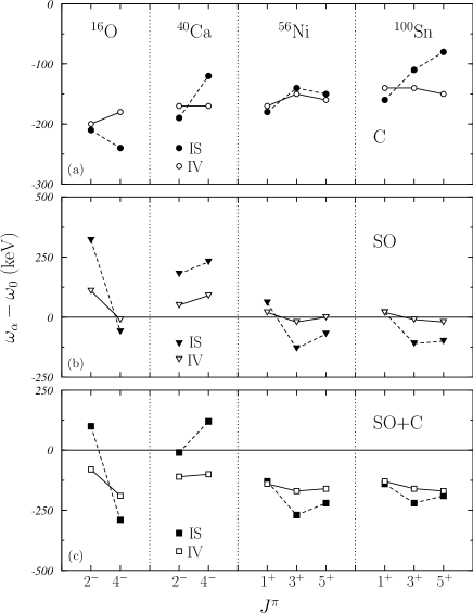
Figure 4: Differences between excitation energies obtained with, $\omega_{\alpha}$, and without, $\omega_{0}$, Coulomb and spin-orbit interactions. In the panel (a) $\omega_{\alpha}$ has been obtained by including the Coulomb interaction only, in the panel (b) the spin-orbit interaction only, and in the panel (c) both of them. The isotopes and the excited states are those listed in Table 1. In each panel, the solid and open symbols indicate the IS and IV results, respectively. The lines are drawn to guide the eyes.

The results shown in the panel (a) of Fig. 4 indicate that the Coulomb interaction is always lowering the excitation energy values, and its effects are rather insensitive to the IS or IV nature of the excitation. In the panel (b) of Fig. 4, we observe , that the effects of the spin-orbit interaction are, in absolute value, always larger in the IS than in the IV excitations. The larger difference between the effects of the spin-orbit interaction on IS and IV excitations occurs for the $2^{-}$ state in ¹⁶O. The sign of the spin-orbit effects is not always the same. We observe an enhancement of the energy values for all the $1^{+}$ and $2^{-}$ states shown in the figure, and also for the $4^{-}$ state in ⁴⁰Ca. For the other cases the energy values are lowered.

We show in the panel (c) of Fig. 4 the global effect obtained by considering both Coulomb and spin-orbit interactions. In the case of IV excitations, we observe a reduction of the energy values of about 150 keV, almost independent of the multipolarity and nucleus considered. The situation for the IS states is more complicated. We find a lowering of the $\omega_{0}$ values in all cases except for the $2^{-}$ state in ¹⁶O and for the two states we have considered in ⁴⁰Ca. In any case, the size of these effects is rather small, reaching $\sim 300$ keV at most. The inclusion of these terms slightly worsen the agreement with the available experimental data, as it is possible to deduce from the results shown in Table 1.

IV.4 Excited states dominated by a specific s.p. transition

In this section we investigate how the effects of the Coulomb and spin-orbit interactions depend on the angular momentum of the excitation. For this study we have selected p-h transitions involving s.p. states near the Fermi energy. When it has been possible we have chosen cases where the particle state is below the continuum threshold. We have calculated all the multipole excitations compatible with the angular momentum coupling of the dominant p-h pair.

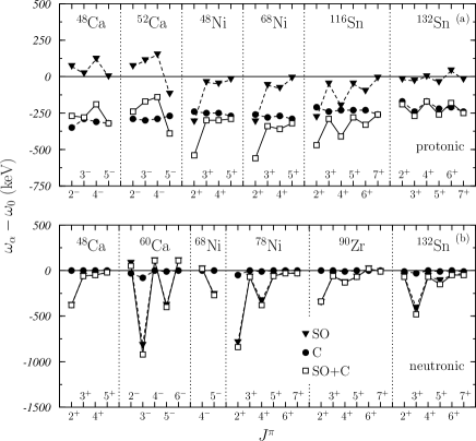
Figure 5: Energy differences between results obtained by selectively including the Coulomb and spin-orbit interactions, and those without them. The various lines connect the results obtained by including only the Coulomb interaction (solid circles), only the spin-orbit interaction (solid triangles) and both of them (open squares). The p-h pairs dominating the various excitations are indicated in Table 2. The lines are drawn to guide the eyes.

		p-h pair
		protons		neutrons
48Ca		$1f_{7/2}\,1d_{3/2}^{-1}$		$2p_{3/2}\,1f_{7/2}^{-1}$
52Ca		$1f_{7/2}\,1d_{3/2}^{-1}$
60Ca				$1g_{9/2}\,1f_{5/2}^{-1}$
48Ni		$2p_{3/2}\,1f_{7/2}^{-1}$
68Ni		$2p_{3/2}\,1f_{7/2}^{-1}$		$1g_{9/2}\,2p_{1/2}^{-1}$
78Ni				$2d_{5/2}\,1g_{9/2}^{-1}$
90Zr				$2d_{5/2}\,1g_{9/2}^{-1}$
116Sn		$2d_{5/2}\,1g_{9/2}^{-1}$
132Sn		$2d_{5/2}\,1g_{9/2}^{-1}$		$2f_{7/2}\,1h_{11/2}^{-1}$

Table 2: Particle-hole pairs dominating the excited states considered in Fig. 5.

A selection of the most relevant results of this investigation is shown in Fig. 5 as difference between the energies obtained by including Coulomb and spin-orbit terms with those obtained without them. We present in Table 2 the p-h pairs dominating the excitations of each nucleus considered in the figure.

We show in the panel (a) of Fig. 5 the results regarding the multipole excitations dominated by proton s.p. pairs. The solid circles indicate the results obtained by considering only the Coulomb interaction, the solid triangles those obtained by considering only the spin-orbit interaction and the open squares those where both interactions have been considered.

We observe that effects of the Coulomb interaction are essentially independent of the multipole excitation, and produce always a lowering of the energy values.

The situation is much more complex for the results obtained with the spin-orbit interaction. For example, in ⁴⁸Ca and ⁵²Ca isotopes we observe an enhancement of the $2^{-}$, $3^{-}$ and $4^{-}$ excitation energies, and a lowering of the energies of the other multipoles considered. We do not identify general trends related to the change of the angular momentum value of the excitation. The combined effect of the Coulomb and spin-orbit interactions is essentially given by the algebric sum of the two effects; the interference phenomena are almost negligible.

The results obtained for the excitations dominated by the neutron s.p. pairs indicated in Table 2 are shown in panel (b) of Fig. 5. In this case, the effect of the Coulomb interaction is almost zero. It is not exactly zero since in the RPA solution, even if dominated by the neutron transition, there are contributions of some proton p-h pairs. As in the proton case, we do not identify general trends related to the inclusion of the spin-orbit interaction. The size of the spin-orbit effects is not always negligible and we observe differences of more than 0.8 MeV for the $3^{-}$ of ⁶⁰Ca and the $2^{+}$ of ⁷⁸Ni.

It is worth noting (see panel (b) of Fig. 5) that those nuclei with the same neutron number show a similar trend in the energy differences for the neutronic excitations. This is apparent for ⁷⁸Ni and ⁹⁰Zr and for the two common excitations of ⁶⁰Ca and ⁶⁸Ni.

V Conclusions

In this paper we have presented the results of a study focused on the role of Coulomb and spin-orbit interactions in RPA calculations. The inclusion of these two terms of the force is required when the s.p. wave functions and energies used in RPA are generated by a HF calculation, to have a complete self-consistency.

We have conducted our investigation in various spherical nuclei covering different regions of the nuclear chart by selecting some low-lying states where the details of the s.p. wave functions around the Fermi surface are relevant.

By studying the low-lying $2^{+}$ and $3^{-}$ excitations we found the need of providing a proper treatment of the exchange term of the Coulomb interaction, usually simulated by the Slater approximation. The exchange term of the Coulomb interaction in RPA calculations generates a globally attractive effect, i. e. an effect which lowers the value of the energies calculated without it. The use of the direct term only has an opposite effect, and the Slater approximation cannot solve the problem.

We have investigated the effects of the Coulomb interaction in IS and IV excitations, and also in excitations dominated by specific p-h pairs and coupled to different angular momentum values. The results of all our calculations confirm the attractive character of the Coulomb interaction. The size of the effects of the Coulomb force is rather similar in all the cases we have investigated and it is of about few hundreds of keV.

The situation regarding the spin-orbit force is much more complicated. The study of the low-lying $2^{+}$ and $3^{-}$ states does not show general behavior of the spin-orbit effects, even though in the great majority of the cases the total effect is attractive. We found a generally larger sensitivity to the IS transitions than to the IV ones, however, we did not observe a general trend of the effects. The sign of the effect changes depending on the nucleus and on the multipolarity investigated. We observed an analogous situation also when we investigated excitations related to specific s.p. pairs. Also in this case, sign and size of the effect depend on the nucleus investigated and on the angular momentum of the excitation.

The effects of the spin-orbit interaction are larger than those of the Coulomb interaction. The energy difference with respect to the results obtained without them can be larger than 1 MeV. The size of the total effect obtained by including both Coulomb and spin-orbit forces in a unique RPA calculation is essentially given by the sum of the two separated results. Interference effects are negligible.

We have also studied the possibility of identifying Coulomb and spin-orbit effects in other observables, different from the excitation energies, but we found very small effects, therefore we did not show here these results.

Self-consistent mean-field models are the starting ground to make predictions about the structure of exotic nuclei. The total self-consistency of these calculations is a requirement which reinforces the reliability of these calculations. The exclusion of the Coulomb and spin-orbit terms of the interaction can generate errors up to about 1 MeV on the RPA excitation energies.

Appendix A The spin-orbit matrix elements

In this appendix, we give some details of our calculations of the RPA matrix elements for the spin-orbit interaction terms $\widehat{V}_{7}$ and $\widehat{V}_{8}$ in Eqs. (1) and (2). We calculate, first, the generic matrix elements

$$\langle\widehat{V}_{7}\rangle\,\equiv\,\langle(ab)J_{1}M_{1}|\widehat{V}_{7}(1,2)|(cd)J_{2}M_{2}\rangle\,\langle(\frac{1}{2}t_{a})\,(\frac{1}{2}t_{b})|\mathbb{1}|(\frac{1}{2}t_{c})\,(\frac{1}{2}t_{d})\rangle\,,$$ (18)

where $a$, $b$, $c$ and $d$ indicate all the quantum numbers identifying the s.p. states involved: the principal quantum number $n$, the orbital angular momentum $l$ and the total angular momentum $j$. In addition, $t_{i}=\pm 1/2$ indicates the third component of the isospin of the $i$-th s.p. state. The explicit expression of the spin-orbit channel of the interaction, $\widehat{V}_{7}$, is:

$$\widehat{V}_{7}(1,2)\,=\,v_{7}(r_{12})\,{\bf L}_{12}\cdot{\bf S}\,.$$ (19)

From the definitions (4)-(6), ${\bf L}_{12}$ can be expressed as:

$${\bf L}_{12}=\frac{1}{2}({\bf L}-{\bf r}_{1}\times{\bf p}_{2}-{\bf r}_{2}\times{\bf p}_{1})\,,$$ (20)

where

$${\bf L}\,=\,{\bf l}_{1}+{\bf l}_{2}\,,$$ (21)

with ${\bf l}_{i}={\bf r}_{i}\times{\bf p}_{i}$. We express the matrix element of (18) as:

$$\langle\widehat{V}_{7}\rangle\,=\,\frac{1}{2}\,\left(V_{LS}\,-\,V_{12}\,-\,V_{21}\right)\,\delta_{t_{a},t_{c}}\,\delta_{t_{b},t_{d}}\,,$$ (22)

where

$$V_{LS}\,=\,\langle(ab)J_{1}M_{1}|v_{7}(r_{12})\,\mathbf{L}\cdot\mathbf{S}|(cd)J_{2}M_{2}\rangle\,,$$ (23)

$$V_{ij}\,=\,\langle(ab)J_{1}M_{1}|v_{7}(r_{12})\,\mathbf{r}_{i}\times\mathbf{p}_{j}\cdot\mathbf{S}|(cd)J_{2}M_{2}\rangle$$ (24)

and the $\delta$’s come from the isospin matrix element.

As suggested in Ref. nak02 , we calculate $V_{LS}$ by changing from $jj$ to $LS$ coupling scheme:

$$V_{LS} = \sum_{L_{1}S_{1}L_{2}S_{2}}\,\hat{j_{a}}\,\hat{j_{b}}\,\hat{L_{1}}\,\hat{S_{1}}\,\hat{j_{c}}\,\hat{j_{d}}\,\hat{L_{2}}\,\hat{S_{2}}\,\left\{\begin{array}[]{ccc}l_{a}&\frac{1}{2}&j_{a}\\ l_{b}&\frac{1}{2}&j_{b}\\ L_{1}&S_{1}&J\end{array}\right\}\,\left\{\begin{array}[]{ccc}l_{c}&\frac{1}{2}&j_{c}\\ l_{d}&\frac{1}{2}&j_{d}\\ L_{2}&S_{2}&J\end{array}\right\}$$ (31)

$$\langle(l_{a}l_{b})L_{1},(\frac{1}{2}\frac{1}{2})S_{1};J_{1}M_{1}|v_{7}(r_{12})\,\mathbf{L}\cdot\mathbf{S}|(l_{c}l_{d})L_{2},(\frac{1}{2}\frac{1}{2})S_{2};J_{2}M_{2}\rangle\,\,,$$ (32)

where we have used the Wigner 9-j symbol and, for the angular momentum indexes, the convention $\hat{l}=\sqrt{2l+1}$. This coupling scheme is convenient because the states are eigenstates of the $\mathbf{L}\cdot\mathbf{S}$ operator. By using this property, we obtain:

$$V_{LS} = \sum_{L_{1}S_{1}L_{2}S_{2}}\,\hat{j_{a}}\,\hat{j_{b}}\,\hat{j_{c}}\,\hat{j_{d}}\,\hat{L_{1}}\,\hat{S_{1}}\,\hat{L_{2}}\,\hat{S_{2}}\,\frac{J_{2}(J_{2}+1)-L_{2}(L_{2}+1)-S_{2}(S_{2}+1)}{2}\,\left\{\begin{array}[]{ccc}l_{a}&\frac{1}{2}&j_{a}\\ l_{b}&\frac{1}{2}&j_{b}\\ L_{1}&S_{1}&J_{1}\end{array}\right\}$$ (40)

$$\left\{\begin{array}[]{ccc}l_{c}&\frac{1}{2}&j_{c}\\ l_{d}&\frac{1}{2}&j_{d}\\ L_{2}&S_{2}&J_{2}\end{array}\right\}\,\langle(l_{a}l_{b})L_{1},(\frac{1}{2}\frac{1}{2})S_{1};J_{1}M_{1}|v_{7}(r_{12})|(l_{c}l_{d})L_{2},(\frac{1}{2}\frac{1}{2})S_{2};J_{2}M_{2}\rangle\,.$$

If $S_{2}=0$, $J_{2}=L_{2}$ and $J_{2}(J_{2}+1)-L_{2}(L_{2}+1)-S_{2}(S_{2}+1)=0$. Thus, the only term contributing to the sum on $S_{2}$ is $S_{2}=1$. Taking this into account we have:

$$V_{LS} = \sum_{L_{1}S_{1}L_{2}}\,\hat{j_{a}}\,\hat{j_{b}}\,\hat{j_{c}}\,\hat{j_{d}}\,\hat{L_{1}}\,\hat{S_{1}}\,\hat{L_{2}}\,\sqrt{3}\,\frac{J_{2}(J_{2}+1)-L_{2}(L_{2}+1)-2}{2}\,\left\{\begin{array}[]{ccc}l_{a}&\frac{1}{2}&j_{a}\\ l_{b}&\frac{1}{2}&j_{b}\\ L_{1}&S_{1}&J_{1}\end{array}\right\}$$ (48)

$$\left\{\begin{array}[]{ccc}l_{c}&\frac{1}{2}&j_{c}\\ l_{d}&\frac{1}{2}&j_{d}\\ L_{2}&1&J_{2}\end{array}\right\}\,\langle(l_{a}l_{b})L_{1},(\frac{1}{2}\frac{1}{2})S_{1};J_{1}M_{1}|v_{7}(r_{12})|(l_{c}l_{d})L_{2},(\frac{1}{2}\frac{1}{2})1;J_{2}M_{2}\rangle\,.$$

Now it is useful to consider the expansion in terms of spherical harmonics $Y_{\lambda\mu}$:

$$v_{7}(r_{12})\,=\,4\sqrt{2\pi}\sum_{L}(-1)^{L}\,\hat{L}\,{\cal V}_{L}^{\rm(7)}(r_{1},r_{2})\,[Y_{L}(r_{1})\otimes Y_{L}(r_{2})]^{0}_{0}\,,$$ (49)

where

$${\cal V}_{L}^{(7)}(r_{1},r_{2})\,=\,\int{\rm d}q\,q^{2}\,j_{L}(qr_{1})\,j_{L}(qr_{2})\,\tilde{v}_{7}(q)\,.$$ (50)

The relation between $v_{7}(r_{12})$ and $\tilde{v}_{7}(q)$ is given in eq. (8). Now we can decouple the $LS$ states and obtain:

$$V_{LS} = \frac{3}{\sqrt{2\pi}}\,\delta_{J_{1},J_{2}}\,\delta_{M_{1},M_{2}}\sum_{L_{2}L}(-1)^{L_{2}+L}\,\hat{l_{a}}\,\hat{l_{b}}\,\hat{l_{c}}\,\hat{l_{d}}\,\hat{j_{a}}\,\hat{j_{b}}\,\hat{j_{c}}\,\hat{j_{d}}\,\hat{L_{2}^{2}}\,\hat{L^{2}}\,[J_{2}(J_{2}+1)-L_{2}(L_{2}+1)-2]$$ (64)

$$\left\{\begin{array}[]{ccc}l_{a}&\frac{1}{2}&j_{a}\\ l_{b}&\frac{1}{2}&j_{b}\\ L_{2}&1&J_{2}\end{array}\right\}\,\left\{\begin{array}[]{ccc}l_{c}&\frac{1}{2}&j_{c}\\ l_{d}&\frac{1}{2}&j_{d}\\ L_{2}&1&J_{2}\end{array}\right\}\,\left\{\begin{array}[]{ccc}l_{a}&l_{b}&L_{2}\\ l_{d}&l_{c}&L\end{array}\right\}\,\left(\begin{array}[]{ccc}l_{a}&l_{c}&L\\ 0&0&0\end{array}\right)\,\left(\begin{array}[]{ccc}l_{b}&l_{d}&L\\ 0&0&0\end{array}\right)$$

$$\int{\rm d}r_{1}\,r_{1}^{2}\,R_{a}^{*}(r_{1})\,R_{c}(r_{1})\int{\rm d}r_{2}\,r_{2}^{2}\,{\cal V}_{L}^{\rm(7)}(r_{1},r_{2})\,R_{b}^{*}(r_{2})\,\,R_{d}(r_{2})\,.$$

For the calculation of $V_{12}$ we use again the $LS$ coupling scheme and the operator written as follows:

$${\bf r_{1}}\times{\bf p}_{2}\cdot{\bf S}\,=\,i\,\sqrt{6}\,[[{\bf r}_{1}\otimes{\bf p}_{2}]^{1}\otimes{\bf S}]^{0}_{0}\,.$$ (65)

The matrix element $V_{12}$ is given by:

$$V_{12} = i\,\sqrt{6}\sum_{L_{1}S_{1}L_{2}S_{2}}\,\hat{j_{a}}\,\hat{j_{b}}\,\hat{j_{c}}\,\hat{j_{d}}\,\hat{L_{1}}\,\hat{L_{2}}\,\hat{S_{1}}\,\hat{S_{2}}\,\left\{\begin{array}[]{ccc}l_{a}&\frac{1}{2}&j_{a}\\ l_{b}&\frac{1}{2}&j_{b}\\ L_{1}&S_{1}&J_{1}\end{array}\right\}\,\left\{\begin{array}[]{ccc}l_{c}&\frac{1}{2}&j_{c}\\ l_{d}&\frac{1}{2}&j_{d}\\ L_{2}&S_{2}&J_{2}\end{array}\right\}$$

$$\langle(l_{a}l_{b})L_{1},(\frac{1}{2}\frac{1}{2})S_{1};J_{1}M_{1}|v_{7}(r_{12})\,[[{\bf r}_{1}\otimes{\bf p}_{2}]^{1}\otimes{\bf S}]^{0}_{0}|(l_{c}l_{d})L_{2},(\frac{1}{2}\frac{1}{2})S_{2};J_{2}M_{2}\rangle$$

Decoupling the $LS$ states we obtain:

$$V_{12} = i\,\sqrt{2}\,\delta_{J_{1},J_{2}}\,\delta_{M_{1},M_{2}}\,\sum_{L_{1}S_{1}L_{2}S_{2}}(-1)^{L_{2}+S_{1}+1+J_{2}}\,\hat{j_{a}}\,\hat{j_{b}}\,\hat{j_{c}}\,\hat{j_{d}}\,\hat{L_{1}}\,\hat{L_{2}}\,\hat{S_{1}}\,\hat{S_{2}}\,$$ (82)

$$\left\{\begin{array}[]{ccc}l_{a}&\frac{1}{2}&j_{a}\\ l_{b}&\frac{1}{2}&j_{b}\\ L_{1}&S_{1}&J_{2}\end{array}\right\}\,\left\{\begin{array}[]{ccc}l_{c}&\frac{1}{2}&j_{c}\\ l_{d}&\frac{1}{2}&j_{d}\\ L_{2}&S_{2}&J_{2}\end{array}\right\}\,\left\{\begin{array}[]{ccc}L_{1}&S_{1}&J_{2}\\ S_{2}&L_{2}&1\end{array}\right\}$$

$$\langle(l_{a}l_{b})L_{1}\|v_{7}(r_{12})\,[{\bf r}_{1}\otimes{\bf p}_{2}]^{1}\|(l_{c}l_{d})L_{2}\rangle\,\langle(\frac{1}{2}\frac{1}{2})S_{1}\|{\bf S}\|(\frac{1}{2}\frac{1}{2})S_{2}\rangle\,.$$

By using again the expansion of eq. (49) we have:

$$v_{7}(r_{12})\,[{\bf r}_{1}\otimes{\bf p}_{2}]^{1}_{\mu} = -i\,4\sqrt{2\pi}\sum_{LK_{1}K_{2}}\hat{L}\,\hat{K_{1}}\,\hat{K_{2}}\,\left\{\begin{array}[]{ccc}L&1&K_{1}\\ 1&K_{2}&1\end{array}\right\}\,\left(\begin{array}[]{ccc}L&1&K_{1}\\ 0&0&0\end{array}\right)$$ (88)

$$r_{1}\,{\cal V}_{L}^{\rm(7)}(r_{1},r_{2})\,[Y_{K_{1}}(r_{1})\otimes[Y_{L}(r_{2})\otimes\nabla_{2}]^{K_{2}}]^{1}_{\mu}\,,$$

where $\nabla$ is the gradient operator, and by considering that the spin matrix element is:

$$\langle(\frac{1}{2}\frac{1}{2})S_{1}\|{\bf S}\|(\frac{1}{2}\frac{1}{2})S_{2}\rangle\,=\,\sqrt{6}\,\delta_{S_{1},S_{2}}\,\delta_{S_{1},1}$$ (89)

we have:

$$V_{12} = 18\sqrt{\frac{2}{\pi}}\,\delta_{J_{1},J_{2}}\,\delta_{M_{1},M_{2}}\,\sum_{L_{1}L_{2}}\sum_{LK_{1}K_{2}}(-1)^{l_{a}+l_{d}+L_{2}+J_{2}}\,\hat{l_{a}}\,\hat{l_{b}}\,\hat{l_{c}}\,\hat{l_{d}}\,\hat{j_{a}}\,\hat{j_{b}}\,\hat{j_{c}}\,\hat{j_{d}}\,\hat{L_{1}^{2}}\,\hat{L_{2}^{2}}\,\hat{L^{2}}\,\hat{K_{1}^{2}}\,\hat{K_{2}^{2}}$$ (118)

$$\left\{\begin{array}[]{ccc}l_{a}&l_{b}&L_{1}\\ l_{c}&l_{d}&L_{2}\\ K_{1}&K_{2}&1\end{array}\right\}\,\left\{\begin{array}[]{ccc}l_{a}&\frac{1}{2}&j_{a}\\ l_{b}&\frac{1}{2}&j_{b}\\ L_{1}&1&J_{2}\end{array}\right\}\,\left\{\begin{array}[]{ccc}l_{c}&\frac{1}{2}&j_{c}\\ l_{d}&\frac{1}{2}&j_{d}\\ L_{2}&1&J_{2}\end{array}\right\}\,\left\{\begin{array}[]{ccc}L_{1}&1&J_{2}\\ 1&L_{2}&1\end{array}\right\}\,\left\{\begin{array}[]{ccc}L&1&K_{1}\\ 1&K_{2}&1\end{array}\right\}$$

$$\left(\begin{array}[]{ccc}L&1&K_{1}\\ 0&0&0\end{array}\right)\,\left(\begin{array}[]{ccc}l_{a}&K_{1}&l_{c}\\ 0&0&0\end{array}\right)\int{\rm d}r_{1}\,r_{1}^{3}\,R_{a}^{*}(r_{1})\,R_{c}(r_{1})\,\int{\rm d}r_{2}\,r_{2}^{2}\,R_{b}^{*}(r_{2})\,{\cal V}_{L}^{\rm(7)}(r_{1},r_{2})$$

$$\left\{\left(\begin{array}[]{ccc}l_{d}&K_{2}&l_{b}\\ 0&0&0\end{array}\right)\,\left(\begin{array}[]{ccc}K_{2}&1&L\\ 0&0&0\end{array}\right)\,\frac{\rm d}{{\rm d}r_{2}}\,R_{d}(r_{2})\right.$$

$$\left.+\,\sqrt{2}\,\xi(l_{b}+l_{d}+L+1)\,\sqrt{l_{d}(l_{d}+1)}\,\left(\begin{array}[]{ccc}l_{d}&K_{2}&l_{b}\\ 1&-1&0\end{array}\right)\,\left(\begin{array}[]{ccc}K_{2}&1&L\\ 1&-1&0\end{array}\right)\,\frac{1}{r_{2}}\,R_{d}(r_{2})\right\}\,,$$

where $\xi(n)=1$ or 0 if $n$ is even or odd, respectively.

The expression of $V_{21}$ can be obtained by using the same procedure with the obvious changes.

For the isospin dependent channel,

$$\widehat{V}_{8}(1,2)\,\equiv\,v_{8}(r_{12})\,{\bf L}_{12}\cdot{\bf S}\,\mbox{\boldmath$\tau$}(1)\cdot\mbox{\boldmath$\tau$}(2)\,,$$ (119)

the calculation is similar with the only difference of the isospin matrix element which is now:

$$\langle(\frac{1}{2}t_{a})\,(\frac{1}{2}t_{b})|\mbox{\boldmath$\tau$}(1)\cdot\mbox{\boldmath$\tau$}(2)|(\frac{1}{2}t_{c})\,(\frac{1}{2}t_{d})\rangle =$$

$$2\,\left(\delta_{t_{a},\frac{1}{2}}\,\delta_{t_{b},-\frac{1}{2}}\,\delta_{t_{c},-\frac{1}{2}}\,\delta_{t_{d},\frac{1}{2}}\,+\,\delta_{t_{a},-\frac{1}{2}}\,\delta_{t_{b},\frac{1}{2}}\,\delta_{t_{c},\frac{1}{2}}\,\delta_{t_{d},-\frac{1}{2}}\right)\,+$$

$$\left(\delta_{t_{a},\frac{1}{2}}\,\delta_{t_{c},\frac{1}{2}}\,-\,\delta_{t_{a},-\frac{1}{2}}\,\delta_{t_{c},-\frac{1}{2}}\right)\left(\delta_{t_{b},\frac{1}{2}}\,\delta_{t_{d},\frac{1}{2}}\,-\,\delta_{t_{b},-\frac{1}{2}}\,\delta_{t_{d},-\frac{1}{2}}\right)\,.$$

- (1) J. Terasaki, J. Engel, M. Bender, J. Dobaczewski, W. Nazarewicz, M. Stoitsov, Phys. Rev. C 71 (2005) 034310.
- (2) S. Fracasso, G. Colò, Phys. Rev. C 72 (2005) 064310.
- (3) T. Sil, S. Shlomo, B. K. Agrawal, P. G. Reinhard, Phys. Rev. C 73 (2006) 034316.
- (4) G. Colò, H. Sagawa, S. Fracasso, P. F. Bortignon, Phys. Lett. B 646 (2007) 227.
- (5) C. Losa, A. Pastore, Døssing, E. Vigezzi, R. A. Broglia, Phys. Rev. C 81 (2010) 064307.
- (6) G. Colò, L. Cao, N. Van Giai, L. Capelli, Comp. Phys. Comm. 184 (2013) 142.
- (7) S. Péru, J. F. Berger, P. F. Bortignon, Eur. Phys. J. A 26 (2005) 25.
- (8) V. De Donno, G. Co’, M. Anguiano, A. M. Lallena, Phys. Rev. C 83 (2011) 044324.
- (9) J. C. Slater, Phys. Rev. 81 (1951) 85.
- (10) G. Co’, A. M. Lallena, Phys. Rev. C 57 (1998) 145.
- (11) A. R. Bautista, G. Co’, A. M. Lallena, Nuovo Cimento A 112 (1999) 1117.
- (12) A. L. Fetter, J. D. Walecka, Quantum theory of many-particle systems, McGraw-Hill, San Francisco, 1971.
- (13) P. Ring, P. Schuck, The nuclear many-body problem, Springer, Berlin, 1980.
- (14) J. Suhonen, From nucleons to nucleus, Springer, Berlin, 2007.
- (15) V. De Donno, Nuclear excited states within the random phase approximation theory, Ph.D. thesis, Università del Salento (Italy), http://www.fisica.unisalento.it/gpco/stud.html (2008).
- (16) S. Goriely, S. Hilaire, M. Girod, S. Péru, Phys. Rev. Lett. 102 (2009) 242501.
- (17) J. Dechargé, D. Gogny, Phys. Rev. C 21 (1980) 1568.
- (18) J. F. Berger, M. Girod, D. Gogny, Comp. Phys. Commun. 63 (1991) 365.
- (19) G. Co’, A. M. Lallena, Nuovo Cimento A 111 (1998) 527.
- (20) S. Hilaire, M. Girod, Eur. Phys. J. A 33 (2007) 237.
- (21) C. Titin-Schnaider, P. Quentin, Phys. Lett. B 49 (1974) 397.
- (22) J. Skalski, Phys. Rev. C 63 (2001) 024312.
- (23) J. Le Bloas, M.-H. Koh, P. Quentin, L. Bonneau, J. I. A. Ithnin, Phys. Rev. C 84 (2011) 014310.
- (24) M. Anguiano, J. L. Egido, L. M. Robledo, Nucl. Phys. A 683 (2001) 227.
- (25) C. M. Lederer, V. S. Shirley, Table of isotopes, 7th ed., John Wiley and Sons, New York, 1978.
- (26) Broohaven National Laboratory, National Nuclear Data Center, http://www.nndc.bnl.gov/.
- (27) S. Raman, C. W. Nestor, P. Tikkanen, Atomic Data and Nuclear Data Tables 78 (2001) 1.
- (28) N. J. Stone, Atomic Data and Nuclear Data Tables 90 (2005) 75.
- (29) J. Ziegler, G. A. Peterson, Phys. Rev. 165 (1968) 1337.
- (30) A. Ansari, P. Ring, Phys. Rev. C 74 (2006) 054313.
- (31) B. G.Carlsson, J. Tovainen, A. Pastore, Phys. Rev. C 86 (2012) 014307.
- (32) H. Nakada, M. Sato, Nucl. Phys. A 699 (2002) 511.