$W^{\prime}\to hH^{\pm}$ decay in $G(221)$ models

Abstract

Based on extended $SU(2)_{1}\times SU(2)_{2}\times U(1)_{\text{X}}$ gauge groups, $G(221)$ models predict the existence of an additional heavy gauge boson $W^{\prime}$ and of a heavy charged Higgs boson $H^{\pm}$. Within this model we calculate the coupling of $W^{\prime}$ to the $hH^{\pm}$ pair, where $h$ can be identified with the Standard Model Higgs boson discovered recently at LHC. Using a phenomenological constraint on the ratio of the symmetry breaking scales in $G(221)$ models, the $W^{\prime}\to hH^{\pm}$ decay width and the $hH^{\pm}$ production cross section via an intermediate $W^{\prime}$ in $pp$ collisions at $\sqrt{s}=$ 8 and 14 TeV are calculated. Fiducial cross sections obtained with $G(221)$ models for several final states produced at LHC through the $W^{\prime}\to hH^{\pm}$ decay are compared with recent results in searches for supersymmetry published by the ATLAS Collaboration.

1 Introduction

The discovery at LHC [1] by both ATLAS and CMS of a new massive scalar particle $h$ with properties closely resembling those of the Higgs boson of Standard Model (SM) stimulated the investigation of more general models which predict several, neutral and charged, Higgs bosons, and which should accomodate in a consistent way this discovery.

The $G(221)$ models [2, 3, 4, 5, 6, 7, 8, 9, 10, 11, 12, 13, 14, 15, 16, 17] are a class of models that add one more $SU(2)$ gauge group to the $SU(2)_{L}\times U(1)_{Y}$ gauge structure of the SM. An important prediction of these models is the existence of new heavy $Z^{\prime}$ and $W^{\prime}$ gauge bosons, present also in other extensions of the SM [18, 19]. In $G(221)$ models the symmetry is spontaneously broken twice, giving mass to the new $W^{\prime}$ and $Z^{\prime}$ bosons and to the SM bosons $W$ and $Z$. Depending on the symmetry breaking pattern, there are several versions: left-right symmetric models [2, 3, 5], lepto-phobic, hadro-phobic, fermio-phobic [6, 7, 8], un-unified [13] and non-universal [15, 10, 16]. The Higgs sector is enlarged with a pair of heavy charged Higgs $H^{\pm}$, similar to the two-Higgs doublet-models (2HDM) [20, 21] or supersymmetric theories [22]. In some $G(221)$ models, a consequence is the existence of a $W^{\prime}hH^{\pm}$ interaction, where $h$ stands for a light neutral boson that can be identified with the SM Higgs.

A review of $G(221)$ models and a global analysis of the phenomenological constraints on their parameters from precision data can be found in [23]. More recently, the LHC phenomenology of models with an additional $SU(2)$ group was investigated in [24, 25, 26], while the coupling of $W^{\prime}$ to a pair of odd heavy Higgs particles was studied in [27].

In the present work, we study several final states produced in $pp$ interactions at the LHC through the $W^{\prime}\to hH^{\pm}$ decay, predicted by a class of $G(221)$ models. The aim was to consider new decay channels of the $W^{\prime}$ boson, whose searches were based up to now on its decays to $l\bar{\nu_{l}}$ and quark-antiquark pairs [19, 28, 29, 30]. As a first estimate, we compared the predictions of $G(221)$ models for several fiducial cross sections with selections adopted in searches for SUSY, with the model-independent upper limits on the visible cross-sections for beyond-standard model physics measured by ATLAS [31, 32, 33, 34, 35].

The paper is organized as follows. In section 2 we present the Higgs sector of the $G(221)$ models. In section 3 we briefly discuss the Lagrangian terms of interest for the present study and derive the form of the $W^{\prime}hH^{\pm}$ interaction. Using recent phenomenological constraints on the $G(221)$ models [23], the $W^{\prime}\to hH^{+}$ decay width and the cross section for the $hH^{+}$ inclusive pair production in $pp$ collisions at $\sqrt{s}=$8 and 14  TeV are calculated in section 4. We also give here the total cross section for the production of a final state with two leptons, four jets and missing transverse energy in $pp$ collisions at 8 and 14 TeV. Section 5 is devoted to the study of several final states produced at LHC through the $W^{\prime}\to hH^{+}$ decay. The simulation framework and the kinematical cuts applied in the analysis are described. Finally, we compare the fiducial cross sections calculated with $G(221)$ models with those predicted by 2HDM and with the model-independent upper limits on the visible cross-sections, determined by ATLAS in SUSY searches based on the same final states.

2 Higgs sector of $G(221)$ models

We adopt the symmetry breaking of the $G(221)$ models as discussed in [23]

$$SU(2)_{1}\times SU(2)_{2}\times U(1)_{X}\rightarrow SU(2)_{L}\times U(1)_{Y}\rightarrow U(1)_{em}$$ (1)

by means of two symmetry breaking stages. For the first stage, the hypercharge is $Y=X+T_{3}^{(2)}$. For the second one, $Q=T_{3}^{(1)}+Y/2=T_{3}^{(1)}+(T_{3}^{(2)}+X)/2$. This is the scenario of the left-right (LR) symmetric, lepto-phobic, hadro-phobic and fermio-phobic models. Another scenario, proper to the un-unified and non-universal models, breaks first $SU(2)_{1}\times SU(2)_{2}$ to $SU(2)_{L}$, and then the SM reduction $SU(2)_{L}\times U(1)_{Y}\rightarrow U(1)_{em}$ takes place. The Higgs sector for these scenarios may contain a doublet, a triplet, or a bidoublet Higgs.

We shall consider only the first symmetry breaking pattern, because it predicts a nontrivial coupling between a heavy gauge boson $W^{\prime}$, a neutral light Higgs boson $h$ and a charged Higgs boson $H^{+}$.

For the first symmetry breaking stage we adopt a doublet complex scalar

$$\Phi=\left(\begin{array}[]{c}\phi^{+}\\ \phi^{0}\end{array}\right),$$ (2)

which transforms as $(1,2,\frac{1}{2})$ under the group action and gives masses to the heavy gauge bosons $W^{\prime}$ and $Z^{\prime}$. For the second symmetry breaking stage, we adopt a bidoublet complex scalar $\mathcal{H}$ transforming as $(2,\bar{2},0)$. For fullfiling the charge conservation relation $Q=T_{3}^{(1)}+(T_{3}^{(2)}+X$)/2, it must have the form:

$$\mathcal{H}=\left(\begin{array}[]{c c}h_{1}^{0}&h_{1}^{+}\\ h_{2}^{-}&h_{2}^{0}\end{array}\right).$$ (3)

The doublet and the bidoublet have nonzero vacuum expectation values (v.e.v.):

$$\langle\Phi\rangle=\frac{1}{\sqrt{2}}\left(\begin{array}[]{c}0\\ u\end{array}\right),$$ (4)

and

$$\langle\mathcal{H}\rangle=\left(\begin{array}[]{c c}k&0\\ 0&k^{\prime}\end{array}\right),$$ (5)

where $u$, $k$ and $k^{\prime}$ are real. It is convenient to write the parameters $k$ and $k^{\prime}$ as [23]

$$k=\frac{v\cos\bar{\beta}}{\sqrt{2}},\qquad k^{\prime}=\frac{v\sin\bar{\beta}}{\sqrt{2}},$$ (6)

where $v\approx 246\,\text{GeV}$ according to SM.

The symmetry breaking scale of the first stage is much higher than the electroweak one, therefore the parameter [23]

$${}x\equiv\frac{u^{2}}{v^{2}}$$ (7)

is expected to be very large. In the present study we have adoptod from [23] the phenomenological constraint $x\geq 100$. As remarked in [23, 24], the corrections depending on $\bar{\beta}$ to the observables are numerically suppressed, so this parameter is not constrained by the global-fit analyses. For some of the discussions given below, we assumed that the ratio $k^{\prime}/k$ is small.

The Higgs sector of the model contains 12 real scalars, from which 6 zero-mass modes go into the longitudinal degrees of freedom of $W^{\prime\pm}$, $Z^{\prime}$ in the first symmetry breaking stage, respectively of $W^{\pm}$ and $Z$ in the second one. After the symmetry breakings, 6 physical degrees of freedom remain, from which we will be interested in a neutral SM-like Higgs boson $h$ and a charged Higgs boson $H^{+}$.

3 Lagrangian of $G(221)$ models and $W^{\prime}hH^{\pm}$ interaction

The Lagrangian of $G(221)$ models is invariant under the transformations $\Phi\to\Phi^{\prime}$, $\mathcal{H}\to\mathcal{H}^{\prime}$, where [3]

$$\Phi^{\prime}=U_{2}\Phi,\quad\quad\mathcal{H}^{\prime}=U_{1}\mathcal{H}U_{2}^{\dagger},$$ (8)

with $U_{1}\in SU(2)_{1}$, $U_{2}\in SU(2)_{2}$. We are interested in the kinetic and potential terms of the Lagrangian:

$$\mathcal{L}\sim\Tr\left[(\mathcal{D}_{\mu}\mathcal{H})^{\dagger}(\mathcal{D}^{\mu}\mathcal{H})\right]-V(\mathcal{H},\widetilde{\mathcal{H}},\Phi,\widetilde{\Phi}),$$ (9)

where

$$\mathcal{D}_{\mu}\mathcal{H}=\partial_{\mu}\mathcal{H}-i\,\frac{g_{1}}{2}\,\sum_{j=1}^{3}\tau_{j}W_{j}\mathcal{H}+i\,\frac{g_{2}}{2}\,\mathcal{H^{\dagger}}\sum_{j=1}^{3}\tau_{j}W^{\prime}_{j}$$ (10)

is the covariant derivative that fixes the local gauge interaction, $\tau_{j}$ are the Pauli matrices, and $g_{1}$, $g_{2}$ are the coupling constants for the first and the second symmetry groups. We placed ourselves in the frame of $G(221)$ models which identify the gauge bosons of the groups $SU(2)_{1}$ and $SU(2)_{2}$ with the SM boson $W$ and an additional boson $W^{\prime}$, respectively.

The most general Higgs potential $V$ is written in terms of the fields $\mathcal{H}$, $\widetilde{\mathcal{H}}$, $\Phi$ and $\widetilde{\Phi}$, where $\widetilde{\mathcal{H}}=\tau_{2}\mathcal{H}^{*}\tau_{2}$ and $\widetilde{\Phi}=i\tau_{2}\Phi^{*}$ ($\mathcal{H}^{*}$ and $\Phi^{*}$ denote the complex conjugates). The important remark here is that $\widetilde{\mathcal{H}}$ and $\widetilde{\Phi}$ transform under $SU(2)$ exactly as $\mathcal{H}$ and $\Phi$, respectively [2, 9, 36]. We mention that the original fields in the Lagrangian do not coincide with the physical fields, defined as eigenstates of the mass matrices. Likewise, due to the mixings, the parameters entering $\mathcal{L}$ are not exactly the parameters determined phenomenologically. We shall specify the differences in the cases of interest.

3.1 Higgs potential

We adopt the potential [9, 12]

$$V(\mathcal{H},\widetilde{\mathcal{H}},\Phi,\widetilde{\Phi})=-\mu_{1}^{2}\Tr(\mathcal{H}^{\dagger}\mathcal{H})+\lambda_{1}\,[\Tr(\mathcal{H}^{\dagger}\mathcal{H})]^{2}+\lambda_{2}\Tr(\mathcal{H}^{\dagger}\mathcal{H}\mathcal{H}^{\dagger}\mathcal{H})$$

$$+ \frac{1}{2}\lambda_{3}\,[\Tr(\mathcal{H}^{\dagger}\widetilde{\mathcal{H}})+\Tr(\widetilde{\mathcal{H}}^{\dagger}\mathcal{H})]^{2}+\frac{1}{2}\lambda_{4}\,[\Tr(\mathcal{H}^{\dagger}\widetilde{\mathcal{H}})-\Tr(\widetilde{\mathcal{H}}^{\dagger}\mathcal{H})]^{2}$$

$$+ \lambda_{5}\Tr(\mathcal{H}^{\dagger}\mathcal{H}\widetilde{\mathcal{H}}^{\dagger}\widetilde{\mathcal{H}})+\frac{1}{2}\lambda_{6}\,[\Tr(\mathcal{H}^{\dagger}\widetilde{\mathcal{H}}\mathcal{H}^{\dagger}\widetilde{\mathcal{H}})+\Tr(\widetilde{\mathcal{H}}^{\dagger}\mathcal{H}\widetilde{\mathcal{H}}^{\dagger}\mathcal{H})]$$

$$- \mu_{2}^{2}\Phi^{\dagger}\Phi+\rho_{1}(\Phi^{\dagger}\Phi)^{2}+\alpha_{1}\Tr(\mathcal{H}^{\dagger}\mathcal{H})\Phi^{\dagger}\Phi+\alpha_{2}\Phi^{\dagger}\mathcal{H}^{\dagger}\mathcal{H}\Phi+\alpha^{\prime}_{2}\Phi^{\dagger}\widetilde{\mathcal{H}}^{\dagger}\widetilde{\mathcal{H}}\Phi,$$

where $\mu_{1}$, $\mu_{2}$, $\lambda_{1}\,,\ldots\lambda_{6}$, $\alpha_{1}$, $\alpha_{2}$ and $\alpha^{\prime}_{2}$ are real parameters. We note that $\widetilde{\Phi}$ does not produce new terms in this case.

The equations for the minimum of the potential, which can be written in terms of the v.e.v. of the fields as[9, 12]

$$\frac{\partial V}{\partial u}=\frac{\partial V}{\partial k}=\frac{\partial V}{\partial k^{\prime}}=0,$$ (12)

do not have an unique solution. We adopted the following constraints:

$$\mu_{2}^{2} = \alpha_{1}(k^{2}+k^{\prime 2})+\alpha^{\prime}_{2}k^{2}+\alpha_{2}k^{\prime 2}+\rho_{1}u^{2},$$ (13)

$$\mu_{1}^{2} = 2(\lambda_{1}+\lambda_{2})(k^{2}+k^{\prime 2})+\frac{1}{2}\alpha_{1}u^{2}+\frac{(\alpha^{\prime}_{2}k^{2}-\alpha_{2}k^{\prime 2})u^{2}}{2\Delta k^{2}},$$

$$\lambda_{3} = \frac{1}{4}(\lambda_{2}-\lambda_{5}-\lambda_{6})-\frac{\Delta\alpha u^{2}}{16\Delta k^{2}},$$

where $\Delta\alpha=\alpha_{2}-\alpha^{\prime}_{2}$ and $\Delta k^{2}=k^{2}-k^{\prime 2}$. Using (6), we can replace $k^{2}+k^{\prime 2}=v^{2}/2$.

By inserting this solution in the expression (3.1) of the potential, with the scalar fields in $\Phi$ and $\mathcal{H}$ replaced by their vacuum expectation values (4) and (5), we extract the mass matrix of the charged scalar sector:

$$M_{+}^{2}=\left(\begin{array}[]{ccc}\frac{\Delta\alpha k^{2}u^{2}}{2\Delta k^{2}}&\frac{\Delta\alpha ku}{\sqrt{2}}&\frac{\Delta\alpha kk^{\prime}u^{2}}{2\Delta k^{2}}\\ \frac{\Delta\alpha ku}{\sqrt{2}}&\Delta\alpha\Delta k^{2}&\frac{\Delta\alpha k^{\prime}u}{\sqrt{2}}\\ \frac{\Delta\alpha kk^{\prime}u^{2}}{2\Delta k^{2}}&\frac{\Delta\alpha k^{\prime}u}{\sqrt{2}}&\frac{\Delta\alpha k^{\prime 2}u^{2}}{2\Delta k^{2}}\\ \end{array}\right),$$ (14)

in the basis $h_{1}^{+}$, $\phi^{+}$, $h_{2}^{+}$. The expressions simplify for $k\rightarrow\frac{v}{\sqrt{2}}$, $k^{\prime}\rightarrow 0$. In this limit, investigated in many studies of $G(221)$ models [9, 12, 11], the field $h_{2}^{+}$ is a massless eigenstate absorbed in the charged gauge field. The fields $h_{1}^{+}$ from the bidoublet and $\phi^{+}$ from the doublet are mixed. After the diagonalization of the mass matrix obtained from (14), we obtain another would-be Goldstone boson and a physical charged Higgs boson $H^{+}$, defined as

$$H^{+}=\frac{1}{\sqrt{u^{2}+v^{2}}}(uh_{1}^{+}+v\phi^{+}),\quad\quad\quad m_{H^{+}}^{2}=\frac{1}{2}\Delta\alpha(u^{2}+v^{2}).$$

For the neutral sector, we consider first the real parts of the fields $h_{1}^{0}$, $h_{2}^{0}$ and $\phi^{0}$. In the limit $k\to v/\sqrt{2}$,  $k^{\prime}\to 0$, the field $h_{2,r}^{0}$ decouples from the other fields. The remaining $2\times 2$ mass matrix is written in the basis $h_{1,r}^{0}$, $\phi_{r}^{0}$ as

$$M_{0}^{2}=\left(\begin{array}[]{ccc}2(\lambda_{1}+\lambda_{2})v^{2}&2(\alpha_{1}+\alpha_{2}^{\prime})uv\\ 2(\alpha_{1}+\alpha_{2}^{\prime})uv&2\rho_{1}u^{2}\\ \end{array}\right),$$ (15)

and has the eigenvalues

$$m^{2}_{1,2}=\frac{1}{2}\left(\lambda v^{2}+\rho_{1}u^{2}\mp\sqrt{(\lambda v^{2}+\rho_{1}u^{2})^{2}-4v^{2}u^{2}(\lambda\rho_{1}-\alpha^{2})}\right),$$ (16)

where $\lambda=\lambda_{1}+\lambda_{2}$ and $\alpha=\alpha_{1}+\alpha_{2}^{\prime}$. We define the mass eigenstates $h$ and $H^{0}$ through

$$h_{1,r}^{0}\sim\frac{h}{\sqrt{2}}+\epsilon\,H^{0},\quad\quad\phi_{r}^{0}\sim-\epsilon\,h+\frac{H^{0}}{\sqrt{2}},$$ (17)

where $\epsilon$ is suppressed by the small ratio $v/u$. To leading order in $v^{2}/u^{2}$ the squared masses are

$$m_{h}^{2}\sim\frac{v^{2}}{2}\left(\lambda_{1}+\lambda_{2}-\frac{\alpha_{1}+\alpha_{2}^{\prime}}{\rho_{1}}\right),\quad\quad m_{H^{0}}^{2}\sim\frac{\rho_{1}u^{2}}{2}.$$ (18)

The light boson $h$, whose mass is proportional to the v.e.v. $v$, is assumed to be a SM-like Higgs boson. The neutral Higgs $H^{0}$ and the charged one $H^{+}$ are expected to be heavier, their masses being proportional to the large v.e.v. $u$.

It is of interest to study also the mass matrix for imaginary fields $h_{1,i}^{0}$, $h_{2,i}^{0}$ and $\phi_{i}^{0}$. It turns out that $\phi_{i}^{0}$ is decoupled from the other fields and has zero mass, being absorbed into the gauge bosons degrees of freedom. Moreover, after the diagonalization of the mass matrix we obtain $h_{1,i}\sim\epsilon^{\prime}\,A^{0}+G^{0}$ and $h_{2,i}\sim A^{0}-\epsilon^{\prime}\,G^{0}$, where $A^{0}$ is a heavy CP-odd neutral boson, $G^{0}$ is another Goldstone boson and $\epsilon^{\prime}$ is small in the limit $k^{\prime}\to 0$.

A detailed analysis of the Higgs sector of $G(221)$ models, in particular of the $LR$ symmetric ones, was performed in [9, 12], and more recently in [37, 38]. Due to the large number of free parameters, the $G(221)$ models have a large flexibility in the Higgs sector. Therefore, it is possible to adjust the properties of the light boson $h$ such as to match those of the SM Higgs. Our purpose here was to show that the physical fields are related in a simple way to the original fields in the Lagrangian, which is important for the derivation of the coupling of interest, between the additional gauge boson $W^{\prime}$ and a pair consisting of a charged and a neutral Higgs boson. The derivation is presented in the next subsection.

3.2 $W^{\prime}hH^{+}$ interaction

The coupling of interest is derived from the kinetic part of the Lagrangian (9), which we write explicitly in terms of the charged gauge fields defined by setting $W^{1}_{\mu}=(W^{+}_{\mu}+W^{-}_{\mu})/\sqrt{2}$, $W^{2}_{\mu}=(-W^{+}_{\mu}+W^{-}_{\mu})/(\sqrt{2}i)$ and similarly for $W^{\prime}$. One finds easily a term containing the original fields $h_{1}^{+}$, $h_{1,r}$ and $W^{\prime-}$ of the Lagrangean $\mathcal{L}$. To pass to the physical fields we use the relations $h_{1}^{+}\sim H^{+}$ and $h_{1,r}^{0}\sim h/\sqrt{2}$ which follow from (3.1) and (17) to first order in $v/u$. We also use the $W^{\prime}$-$W$ mixing term [23]

$$\mathcal{L}\sim-\frac{1}{2}\,g_{1}g_{2}v^{2}\cos\bar{\beta}\,\sin\bar{\beta}\,W^{-}_{\mu}W^{\prime+\mu}+h.c.,$$ (19)

which is obtained from (9) by replacing $h_{1}^{0}$ and $h_{2}^{0}$ by their v.e.v. from (5) and (6) and collecting the terms proportional to $W^{-}_{\mu}W^{\prime+\mu}$. For small $\sin\bar{\beta}$, i.e. for $k^{\prime}\to 0$, the $W$-$W^{\prime}$ mixing given in (19) is small, therefore the physical field $W^{\prime}$, defined as in Ref. [23] from the diagonalization of the $W$-$W^{\prime}$ mass matrix, coincides practically with the original $W^{\prime}$ field in the Lagrangian. Thus, we obtain the $W^{\prime\mp}hH^{\pm}$ interaction written in terms of the physical fields as

$$\mathcal{L}\sim-\frac{1}{2}\,ig_{2}W^{\prime-}_{\mu}(h\,\partial^{\mu}H^{+}-H^{+}\,\partial^{\mu}h)+h.c.$$ (20)

It is of interest to investigate also other interactions of $W^{\prime}$ in the adopted model. One possible coupling is that of $W^{\prime}$ to the pair $H^{0}H^{+}$, where $H^{0}$ is a heavy neutral Higgs boson. It arises from the same term $W^{\prime}h_{1,r}h_{1}^{+}$ of the Lagrangean $\mathcal{L}$, which yielded the coupling $hW^{\prime}H^{+}$ of interest. However, from (17) it follows that the contribution of $H^{0}$ to the field $h_{1,r}$ is suppressed by the small ratio $v/u$. Moreover, it turns out that the coupling of $W^{\prime}$ to the field $h_{2,r}^{0}$, which generates another Higgs field, is identically 0.

In the imaginary fields sector, one can check that the only nonzero term in $\mathcal{L}$ is $W^{\prime}h_{1,i}h_{1}^{+}$, while the coupling $W^{\prime}h_{2,i}h_{1}^{+}$ vanishes identically. Using the expression of $h_{1,i}$ in terms of physical fields given the previous subsection, we obtain from the term $W^{\prime}h_{1,i}h_{1}^{+}$ a physical coupling $W^{\prime}A^{0}H^{+}$ suppressed in the limit $k^{\prime}\to 0$.

The couplings of $W^{\prime}$ to the pair $Wh$ or to the SM bosons $WZ$ can proceed through the $W^{\prime}W$ mixing. As shown in [24], for models with the first breaking symmetry pattern adopted here, these couplings are suppressed by the large parameter $u/v$ and vanish identically for $k^{\prime}=0$. The couplings of $W^{\prime}$ to fermions depend on the details of the model. As discussed in [24], the Sequential Standard Model (SSM), where $W^{\prime}$ has the same couplings to fermions as the SM $W$ boson, can be considered as a reference for the $G(221)$ models, since the gauge boson production cross sections are obtained from the corresponding quantities in the SSM by a simple scaling with a factor depending on the couplings.

3.3 Yukawa interactions

Due to the complexity of the Higgs sector, predictions on the interactions between fermions and the additional Higgs bosons are not available in the general frame of $G(221)$ models. As remarked in [23], in these models there are many free parameters in the Yukawa sector, which can lead to interesting flavor phenomena, particularly in the arena of neutrino physics (see, for example [17]).

More detailed predictions are possible in specific models like the left-right symmetric models, where the groups $SU(2)_{1}$ and $SU(2)_{2}$ are identified with $SU(2)_{L}$ and $SU(2)_{R}$, respectively. According to [37, 38], the structure of the Yukawa couplings of the bidoublet Higgs field ${\mathcal{H}}$ in such models is quite different from that of the Higgs fields of 2HDM. For instance, according to Eq. (15) of [38], the ratio of the $H^{+}\bar{t}b$ squared couplings in LR-symmetric models and type II 2HDM [20, 21] writes as:

$$\frac{g^{2}_{\rm LR}}{g^{2}_{\rm 2HDM}}\approx\frac{m_{t}^{2}[(1+\xi^{2})^{2}/(1-\xi^{2})^{2}+4\xi^{2}/(1-\xi^{2})^{2}]}{m_{b}^{2}\tan^{2}\beta+m_{t}^{2}\cot^{2}\beta},$$ (21)

where $\xi\equiv k^{\prime}/k$ in our notation (4), and $\beta$ is the mixing parameter of 2HDM. The ratio (21) is larger than unity except for very small and very large values of $\tan\beta$, and the result is stable for small $\xi\leq 0.1$.

4 Decay width $\Gamma(W^{\prime}\to hH^{+})$

For simplicity, in what follows we shall refer to the $W^{\prime}$ decay into the positively charged Higgs. Using (20), we write the amplitude of this process at tree level as

$$\mathcal{M}=\frac{ig_{2}}{2}\epsilon^{\prime}_{\mu}(p_{1}-p_{2})^{\mu},$$ (22)

where $\epsilon^{\prime}$ is the $W^{\prime}$ polarization 4-vector and $p_{1}$, $p_{2}$ are the momenta of the two final Higgs bosons. We note that angular momentum conservation implies that the two final bosons are produced in a state of orbital momentum 1 in the $W^{\prime}$ rest frame.

The differential decay rate is given by

$$\rmd\Gamma(W^{\prime}\to hH^{+})=|\mathcal{M}_{av}|^{2}\frac{1}{2m_{W^{\prime}}}2\pi^{4}\delta^{4}(P-p_{1}-p_{2})\frac{d^{3}p_{1}d^{3}p_{2}}{(2\pi)^{3}2E_{1}(2\pi)^{3}2E_{2}}\,,$$ (23)

where the squared amplitude averaged over the initial $W^{\prime}$ polarization states is

$$|\mathcal{M}|_{av}^{2}=\frac{g_{2}^{2}}{4}\,\frac{1}{3}\sum_{\epsilon^{\prime}}\epsilon^{\prime}_{\mu}\epsilon^{\prime\nu}(p_{1}-p_{2})^{\mu}(p_{1}-p_{2})_{\nu}.$$ (24)

Using

$$\sum_{\epsilon^{\prime}}\epsilon^{\prime}_{\mu}\epsilon^{\prime\nu}=-g_{\mu\nu}+\frac{P_{\mu}P_{\nu}}{m_{W^{\prime}}^{2}},\quad P=p_{1}+p_{2},$$ (25)

to evaluate (24) and performing the trivial phase space integral of (23), we finally obtain the partial width as

$$\Gamma(W^{\prime}\to hH^{+})=\frac{g_{2}^{2}}{192\pi}\,\frac{\lambda^{3/2}(m^{2}_{W^{\prime}},m^{2}_{H^{+}},m^{2}_{h})}{m_{W^{\prime}}^{5}},$$ (26)

in terms of the standard kinematical function

$$\lambda(a,b,c)=a^{2}+b^{2}+c^{2}-2ab-2ac-2bc.$$ (27)

A constraint on the coupling $g_{2}$ entering (26) can be derived by writing the mass of $W^{\prime}$ as [23]

$$m^{2}_{W^{\prime}}=\frac{1}{4}g_{2}^{2}u^{2}+\frac{1}{4}g_{2}^{2}v^{2}+\frac{g^{2}_{1}v^{4}\sin^{2}2\bar{\beta}}{4u^{2}},$$ (28)

where the first two terms are the contributions to the mass after the first and second symmetry breaking stages, and the third term is a correction from the $W^{\prime}$-$W$ mixing (19). By neglecting the last term due to the large $u$ in the denominator and using the ratio defined in (7), we write (28) as

$$m_{W^{\prime}}^{2}=\frac{1}{4}g_{2}^{2}v^{2}(x+1),$$ (29)

from which we obtain, to leading order in the large parameter $x$,

$$g_{2}\approx\frac{2m_{W^{\prime}}}{v\sqrt{x}}.$$ (30)

Using this estimate in (26), we obtain

$$\Gamma(W^{\prime}\to hH^{+})=\frac{\lambda^{3/2}(m^{2}_{W^{\prime}},m^{2}_{H^{+}},m^{2}_{h})}{48\pi xv^{2}m^{3}_{W^{\prime}}}=\frac{G_{F}}{24\sqrt{2}\pi x}\frac{\lambda^{3/2}(m^{2}_{W^{\prime}},m^{2}_{H^{+}},m^{2}_{h})}{m^{3}_{W^{\prime}}}.$$ (31)

Table 1: Partial width $\Gamma(W^{\prime}\to hH^{+})$, in GeV, calculated from (31) as a function of $m_{W^{\prime}}$, for three value of the parameter $x$ and $m_{H^{+}}=300\,(500)\,\text{GeV}$.

$m_{W^{\prime}}$[GeV]	$x=100$		$x=500$		$x=1000$
	300	500	300	500	300	500
1000	0.77	0.41	0.15	0.08	0.08	0.04
1500	3.16	2.49	0.64	0.50	0.32	0.25
2000	8.00	7.05	1.61	1.42	0.81	0.71
2500	16.10	14.87	3.25	2.99	1.62	1.50
3000	28.27	26.77	5.69	5.39	2.85	2.70
3500	45.32	43.55	9.14	8.78	4.57	4.39
4000	68.07	66.03	13.72	13.31	6.87	6.66
4500	97.32	95.02	19.63	19.16	9.82	9.59
5000	133.90	131.33	26.99	26.48	13.51	13.25

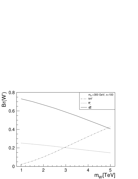
Figure 1: $W^{\prime}$ branching fractions, including the $W^{\prime}\to hH^{+}$ decay.

Several values of $\Gamma(W^{\prime}\to hH^{+})$ calculated using (31) are given in Table 1. We adopted the lower bound $x\geq 100$ derived from recent phenomenological studies [23] of $G(221)$ models. The mass of the light Higgs was set to $m_{h}=126\,\text{GeV}$. Lower limits on the $W^{\prime}$ mass were obtained recently at LHC from the investigation of $W^{\prime}$ decays into leptons [28, 29] and quark-antiquark pairs [30]. The most stringent limit, of 3.8 TeV, is set by the CMS Collaboration [29], by assuming a “sequential” $W^{\prime}$, which has the same couplings to quarks and leptons as the SM $W$ boson. However, when other models and other possible decays of $W^{\prime}$ are considered, the existing limits may be relaxed [27]. Therefore, in our study we considered a larger interval of masses, between 1 and 5 TeV. As for the mass of the charged Higgs boson, limits have been derived recently at LHC [39]. Also, stringent constraints on $m_{H^{+}}$ were derived from $B$ decays in the frame of type II 2HDM by Belle and BABAR [40]. We adopted for $m_{H^{+}}$ two values compatible with these limits.

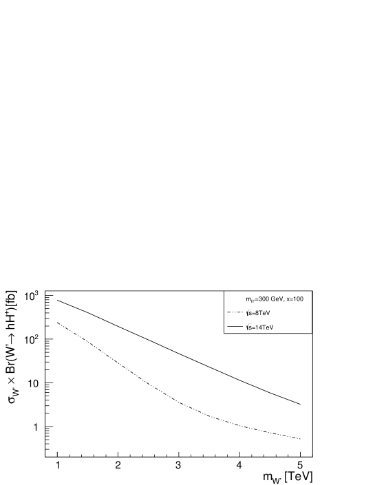
Figure 2: Cross section (in fb) of inclusive production of a $hH^{+}$ pair via the $W^{\prime}\to hH^{+}$ decay in $pp$ collisions at 8 and 14 TeV.

In Fig. 1 we present the branching fractions ${\rm Br}(W^{\prime}\to XY)$, using for the leptonic and quark channels the SSM [18]. The $q\bar{q^{\prime}}$ channel includes $t\bar{b}$. As discussed in the previous section, other decays of $W^{\prime}$ possible in the frame of $G(221)$ models, like $W^{\prime}\to H^{0}H^{+}$, $W^{\prime}\to A^{0}H^{+}$, $W^{\prime}\to WZ$ or $W^{\prime}\to hW$ are suppressed and can be neglected in the approximation of large $u/v$ and small $k^{\prime}$.

We computed also the inclusive cross section for $hH^{+}$ pair production in $pp$ collisions, given by $\sigma_{prod}^{W^{\prime}}\times{\rm Br}(W^{\prime}\to hH^{+})$. The $W^{\prime}$ production cross section in $pp$ collisions was calculated in [41] for various couplings at NLO in QCD. We computed $\sigma_{prod}^{W^{\prime}}$ with PYTHIA LO SSM implementation, with the parton distribution functions for the proton set to CTEQ 5L [42]. The results are presented in Fig. 2, where we show the cross section for the $hH^{+}$ production in $pp$ collisions at $\sqrt{s}=$ 8 and 14 TeV, for $m_{H^{+}}=300\,\text{GeV}$ and $x=100$.

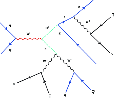
Figure 3: Production of the final state with 2 same-sign leptons, 4 jets and ${\rm E_{T}^{miss}}$ in $pp$ collisions via the $W^{\prime}\to hH^{+}$ decay.

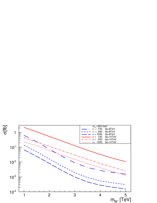
Figure 4: Cross section $\sigma$ (in fb) for the production of 2 electrons, 4 jets and $E_{\rm T}^{\rm miss}$ via the $W^{\prime}\rightarrow hH^{+}$ channel in $pp$ collisions at 8 and 14 TeV.

For illustration, we consider also the production of 2 leptons, 4 jets and ${\rm E_{T}^{miss}}$ in $pp$ collisions via the $W^{\prime}\to hH^{\pm}$ decay (one possible diagram is shown in Fig. 3). In Fig. 4 we present the total cross section for the production of this final state, calculated with the PYTHIA 6.4 in which we implemented the new channel $W^{\prime}\to hH^{\pm}$. Details on the simulations will be given in the next section.

5 Final state comparison study

For several final states, we present a comparison study between the predictions of $G(221)$ models and the experimental upper limits on the visible cross sections determined by ATLAS in SUSY searches. We first describe the simulation procedure and then discuss the specific final state analysis.

5.1 Simulation framework

The simulation and the analysis were based on a framework [43] that chains different software packages together: Monte Carlo generators, programs for the simulation of the events through the detector and programs for data analysis. Using PYTHIA 6.4 as Monte Carlo event generator, we produced data samples for final states which comprise leptons, jets and missing transverse energy. The parton distribution functions set for the proton was CTEQ 5L and the center of mass energy for the $pp$ collisions was set to $8\,\text{TeV}$.

As we mentioned above, PYTHIA 6.4 adopts as default the SSM, where the $W^{\prime}$ boson has the same couplings to fermions as the SM boson $W$. We have implemented in PYTHIA 6.4 the additional $W^{\prime}\to hH^{+}$ channel, with the decay width and the branching ratio set according to the calculations presented in Section 4. We allowed $h$ to decay to $WW$, $ZZ$ and $b\bar{b}$, while the charged Higgs was set to decay as $H^{+}\to t\bar{b}$ in all cases. The top mass was fixed at $172.5$ GeV and the light Higgs mass $m_{h}=126\,\text{GeV}$. All the calculations in this section were performed with $m_{W^{\prime}}=1\,\text{TeV}$, $m_{H^{+}}=300\,\text{GeV}$ and $x=100$.

The default coupling for $H^{+}\to t\bar{b}$ decay in PYTHIA 6.4 is the 2HDM coupling with $\tan\beta=5$, which may underestimate by a large factor the $G(221)$ couplings, as discussed in [37, 38] in the context of the left-right symmetric models. In order to work with a more realistic coupling, we performed the simulations in PYTHIA with the choice $\tan\beta=1$, when the ratio given in (21) is close to 1 for small values of $\xi$. For other decays involved in the production of the final states we assumed SM couplings.

For the comparison with the published results of the ATLAS Collaboration, we used the Delphes framework [44] which provides a realistic fast simulation of the ATLAS detector [45] and delivers reconstructed physics objects, such as leptons, jets, photons and missing energy. The data analysis was performed with ROOT [46].

5.2 Fiducial cross section comparison for various final state topologies

The aim of this section is to compare the predictions of the $G(221)$ models with the recently published results from SUSY searches by the ATLAS Collaboration [31, 32, 33, 34]. Several topologies were investigated in these searches: events containing no leptons, six jets and missing transverse energy $E_{\text{T}}^{\text{miss}}$ [31], one lepton, six jets and $E_{\text{T}}^{\text{miss}}$ [32], two opposite-sign leptons, four jets and $E_{\text{T}}^{\text{miss}}$ [33] and one lepton, four b-jets and $E_{\text{T}}^{\text{miss}}$[34].

In the frame of $G(221)$ models, the same states can be produced in $pp$ collisions via the intermediate $W^{\prime}\to hH^{+}$ decay, with $h\to W^{+}W^{-}$, $ZZ$ or $b\bar{b}$, and $H^{+}\rightarrow t\bar{b}$. The total cross sections for the final states with 0l+ 6j+$E_{\text{T}}^{\text{miss}}$, 1e+6j+$E_{\text{T}}^{\text{miss}}$, 2e+4j+$E_{\text{T}}^{\text{miss}}$ and 1e+4bj+$E_{\text{T}}^{\text{miss}}$, obtained through the production and decay of $W^{\prime}$ with the parameters specified above, are 0.92, 3.96, 0.63 and 10.94 fb, respectively.

Of interest are the cross sections obtained after suitable kinematical cuts, which suppress the background and favor the signal. In the ATLAS studies [31, 32, 33, 34], the kinematical cuts imposed on the final state particles were designed such as to favor SUSY searches. These cuts may be non-optimal for $W^{\prime}$ detection, where all the final states originate from a high-energy particle of large mass. In fact, it turns out that a small number or even no events generated by the simulations based on $G(221)$ models remain after applying the SUSY inspired selections.

In our study, the kinematical cuts on $p_{\text{T}}$, $E_{\text{T}}^{\text{miss}}$ and the pseudorapidity $\eta$ are only a part of the ATLAS SUSY searches set of conditions. No cuts were applied on the transverse mass $m_{\text{T}}$, on the inclusive effective mass $m_{eff}^{inc}$, which is the sum of the transverse momenta of the jets and leptons and the $E_{\text{T}}^{\text{miss}}$, or on the ratio between transverse mass and effective mass ($m_{\text{T}}$/$m_{eff}$). There are also several other variables, like the cotransverse mass $m_{\text{CT}}$ of two $b$-jets, the $p_{\text{T}}$ scalar sum $H_{\text{T}}$ of all jets, the invariant mass of two leptons coming from a $Z$ boson, or the angle between two leptons, which were not constrained in our analysis. Of course, more kinematical cuts applied on the phase space and the consideration of efficiency reconstruction will further reduce the fiducial cross sections.

The zero leptons, six jets and $E_{\text{T}}^{\text{miss}}$ SUSY final state cross-section is set for tight conditions [31]. Thus we require at least six jets with $p_{\rm T}$ greater than 130 GeV for the first one, and greater than 60 GeV for the other five, and $E{\rm{}_{T}^{miss}}$ greater than 160 GeV. The main source of this signature is the pair production of light squarks, each of whom decays through an intermediate chargino to a quark, a $W$ boson and the lightest neutralino, in the MSUGRA/CMSSM model.

The one lepton, six jets and $E_{\text{T}}^{\text{miss}}$ channel is considered for binned hard-single lepton channel [32]. The number of leptons is exactly one, whereas the number of jets at least six. We set $E{\rm{}_{T}^{miss}}>350\,\text{GeV}$, lepton $p_{\text{T}}$ greater than 25 GeV, and the $p_{\rm T}$ of jets greater than 80 and 50 GeV for the first two, respectively greater than 40 GeV for the other jets. This state appears in the gluino inspired MSUGRA model, where a pair of gluinos decay to quarks, a $W$ boson and a neutralino.

For the final state with two opposite-sign leptons, four jets and $E_{\text{T}}^{\text{miss}}$ we require at least two isolated opposite-sign leptons and four jets, with $p_{\text{T}}$ of the leading leptons greater than $25$ GeV and $p_{\text{T}}$ of the leading jets greater than $30$ GeV [33]. This final state was studied in the Gauge Mediated Symmetry Breaking (GMSB), where stop quark is decaying to top and neutralino. Because the neutralino is not considered the lightest SUSY particle (LSP), it could decay into a $Z$ or the SM-like Higgs boson and a gravitino.

The last final state considered consists of one lepton, four $b$-jets and $E{\rm{}_{T}^{miss}}$ [34]. We require exactly one lepton with $p_{\rm T}$ greater than 25 GeV, and at least four jets with $p_{\rm T}$ greater than 80 GeV. The $E{\rm{}_{T}^{miss}}$ has to be greater than 250 GeV. This state is the feature of gluino to quark-antiquark and neutralino decay models. The pseudorapidity regions for the leptons and jets are always $|\eta_{leptons}|<2.47$ and $|\eta_{jets}|<2.7$, according to the ATLAS detector acceptance.

In Table 2 we present the fiducial $G(221)$ model cross-sections, $\sigma_{fid}=\sigma_{prod}\times A$, where $\sigma_{prod}$ is the production cross-section and $A$ is the acceptance of the detector, which includes the kinematical cuts over the phase space. The comparison with the total cross sections given above shows the drastic effect of the kinematical cuts on the final states produced through the decay of $W^{\prime}$. For completeness, the cross sections corresponding to the channel $pp\to W\to hH^{+}$ calculated with PYTHIA 6.4 in the frame of 2HDM are also shown. We indicated separately the contributions of the channels with $WWW$, $ZZW$ and $4bjW$ intermediate states, obtained from $h$ decaying to $WW$, $ZZ$ and $b\bar{b}$, respectively. The fiducial cross sections predicted by the $G(221)$ models are considerably larger than those predicted by 2HDM with the default PYTHIA 6.4 parameters.

In Table 2 we give also the observed 95% CL upper limits on the visible cross section $\sigma_{\rm vis}^{\rm obs}$ of beyond SM processes, determined by ATLAS from experimental measurements with selections for SUSY searches. These are much larger than the fiducial cross sections of the processes involving the production and decay of $W^{\prime}$. However, this result may be due to the use of selections that are not optimal for $W^{\prime}$ detection. Moreover, the observed limits on the visible cross sections offer only a model independent indication on the magnitude of new physics contributions. Detailed studies are necesary to identify proper kinematical cuts for the final states produced by the $W^{\prime}$ decay and to set limits on model parameters from measured data and the SM background in suitable signal regions.

Table 2: Fiducial cross sections (in fb) with selections from SUSY searches, calculated in $G(221)$ for $m_{W^{\prime}}=1000\,\text{GeV},\,m_{H^{+}}=300\,\text{GeV},\,m_{h}=126\,\text{GeV}$ and $x=100$. For comparison, the 2HDM predictions for the same final states are also shown. In the second column we give the observed 95% CL upper limits on new physics cross sections derived by ATLAS in SUSY searches [31, 32, 33, 34].

Final state	ATLAS	$G(221)_{WWW}$	$G(221)_{ZZW}$	$G(221)_{4bjW}$	2HDMWWW	2HDMZZW	2HDM4bjW
$0l,\,6j,\,E_{\text{T}}^{\text{miss}}$	$0.41$	-	$3.11\cdot 10^{-3}$	-	-	$6.05\cdot 10^{-6}$	-
$e,6j,\,E_{\text{T}}^{\text{miss}}$	$0.33$	$3.01\cdot 10^{-4}$	$1.08\cdot 10^{-5}$	-	$3.08\cdot 10^{-7}$	$3.8\cdot 10^{-8}$	-
$\mu,6j,\,E_{\text{T}}^{\text{miss}}$	$0.35$	$1.67\cdot 10^{-4}$	$2.05\cdot 10^{-6}$	-	$3.07\cdot 10^{-7}$	$8\cdot 10^{-9}$	-
$ee,4j,\,E_{\text{T}}^{\text{miss}}$	$0.17$	$2.57\cdot 10^{-2}$	$1.29\cdot 10^{-2}$	-	$2.07\cdot 10^{-4}$	$5.94\cdot 10^{-5}$	-
$e\mu,4j,\,E_{\text{T}}^{\text{miss}}$	-	-	-	-	-	-	-
$\mu\mu,4j,\,E_{\text{T}}^{\text{miss}}$	$0.17$	$1.08\cdot 10^{-2}$	$5.49\cdot 10^{-3}$	-	$8.47\cdot 10^{-5}$	$2.85\cdot 10^{-5}$	-
$e,4bj,\,E_{\text{T}}^{\text{miss}}$	$1.69$	-	-	$7.57\cdot 10^{-3}$	-	-	$1.46\cdot 10^{-5}$
$\mu,4bj,\,E_{\text{T}}^{\text{miss}}$	$1.09$	-	-	$5.56\cdot 10^{-3}$	-	-	$2.14\cdot 10^{-5}$

6 Summary and conclusions

In this paper we studied the $W^{\prime}\to hH^{+}$ decay predicted by some $G(221)$ models [2, 3, 4, 5, 6, 7, 8, 9, 10, 11, 12, 13, 14, 15, 16, 17, 37, 38, 23, 24]. The aim was to compare the predictions of $G(221)$ models for several fiducial cross sections with the model-independent upper limits derived by ATLAS in SUSY searches based on the same final states.

We considered $G(221)$ models with two-stage symmetry breaking, with a scalar sector consisting of a complex doublet in the first stage and of a complex bidoublet in the second. Due to the large number of free parameters, the $G(221)$ models have a great flexibility in the Higgs and Yukawa sectors. Therefore, the properties of the light neutral Higgs boson $h$ can be adjusted to match the properties of the SM Higgs. In the present study we adopted the phenomenological constraint $x\geq 100$ for the parameter defined in (7) and the assumption that the ratio $k^{\prime}/k$ of the vacuum expectation values (5) is small. In this general frame, we calculated the coupling between a heavy charged gauge boson $W^{\prime}$, the light neutral SM-like Higgs boson $h$ and a charged non-standard Higgs boson $H^{\pm}$. We also calculated the partial width $\Gamma(W^{\prime}\to hH^{+})$, the $W^{\prime}$ branching fractions including the $W^{\prime}\to hH^{+}$ channel and the cross section for the inclusive production of the $hH^{+}$ state in $pp$ collisions at 8 and 14 TeV.

We considered also several specific final states produced in $pp$ collisions at the LHC through the $W^{\prime}\to hH^{+}$ decay. We used a simulation framework [43] that chains PYTHIA 6.4 Monte Carlo generator, the Delphes framework for a fast simulation of the ATLAS detector and ROOT for the data analysis. The branching ratios and the total cross-sections for the final states were obtained at LO with PYTHIA 6.4, where we have implemented the new decay channel $W^{\prime}\to hH^{+}$ predicted by $G(221)$ models. The analysis involved specific $p_{\text{T}}$, $\eta$ and $E_{\text{T}}^{\text{miss}}$ selection cuts that were employed by the searches for supersymmetry performed by the ATLAS Collaboration [31, 32, 33, 34, 35]. Our study shows that, assuming specific kinematical cuts that were optimized for SUSY searches by the ATLAS Collaboration, $G(221)$ model fiducial cross sections are larger than those predicted by 2HDM, but considerably below the ATLAS model independent upper limits on new physics cross sections in the corresponding signal regions. Further studies are necessary in order to identify proper kinematical cuts for the final states produced by the decay of $W^{\prime}$ and to set limits on model parameters from measured data and the SM background in suitably defined signal regions.

References

References

- [1] G. Aad et al. (ATLAS Collaboration) 2012 Phys. Lett.B 716 1; S. Chatrchyan et al. (CMS Collaboration) 2012 Phys. Lett.B 716 30
- [2] Mohapatra R N and Pati J C 1975 Phys. Rev.D 11 2558
- [3] Mohapatra R N and Pati J C 1975 Phys. Rev.D 11 566
- [4] Mohapatra R N and Senjanovic G 1981 Phys. Rev.D 23 165
- [5] Pati J C and Salam A 1973 Phys. Rev. Lett.31 661
- [6] Chivukula R S, Coleppa B, Di Chiara S, Simmons E H, He H J, Kurachi M and Tanabashi M D 2006 Phys. Rev.D 74 075011
- [7] Barger V D, Keung W Y and Ma E 1980 Phys. Rev.D 22 727
- [8] Barger V D, Keung W Y and Ma E 1980 Phys. Rev. Lett.44 1169
- [9] Senjanovic G 1979 Nucl. Phys.B 153 334-64
- [10] Li X and Ma E 1981 Phys. Rev. Lett.47 1788
- [11] Cocolicchio D and Fogli G L 1985 Phys. Rev.D 32 3020
- [12] Gunion G F, Grifols J, Mendez A, Kayser B and Olness F 1989 Phys. Rev.D 40 1546
- [13] Georgi H, Jenkins E E and Simmons E H 1990 Nucl. Phys.B 331 541-5
- [14] Cocolicchio D, Fogli G L and Terron J 1991, Phys. Lett.B 255 599
- [15] Malkawi E, Tait T M P and Yuan C P 1996 Phys. Lett.B 385 304
- [16] He X G and Valencia G 2002 Phys. Rev.D 66 013004 [Erratum-ibid. D 66, 079901 ]
- [17] Mohapatra R N et al. 2007 Rept. Prog. Phys. 70 1757 [arXiv:hep-ph/0510213]
- [18] Altarelli G, Mele B and Ruiz-Altaba M 1989 Z. Phys.C 45 109
- [19] J. Beringer et al. (Particle Data Group) 2012 Phys. Rev.D 86 010001
- [20] Branco G C, Ferreira P M, Lavoura L, Rebelo M N, Sher M and Silva J P 2012 Phys. Rept 516 1-102
- [21] Chen C-Y and S. Dawson S 2013 Phys. Rev.D 87 055016
- [22] Gunion J F and Haber H E , 1986 Nucl. Phys.B272 1-76
- [23] Hsieh K, Schmitz K, Yu J-H, Yuan C P 2010 Phys. Rev.D 82 035011 [arXiv:1003.3482]
- [24] Cao Q-H, Li Z, Yu J-H and Yuan C P 2012 Phys. Rev.D 86 095010 [arXiv:1205.3769]
- [25] Schmaltz M and Spethmann C 2011 JHEP 1107:046
- [26] Jezo T, Klasen M and Schienbein I, 2012 Phys. Rev.D 86 035005
- [27] Dobrescu B A and Peterson A D 2013 Fermilab-PUB-13-549-T, arXiv:1312.1999
- [28] G. Aad et al., ATLAS Collaboration 2011 Phys. Lett.B 705 28–46
- [29] CMS Collaboration 2013 Search for leptonic decays of bosons in pp collisions at , report CMS-PAS-EXO-12-060, March 2013
- [30] ATLAS Collaboration 2013, ATLAS-CONF-2013-050
- [31] ATLAS Collaboration 2013, ATLAS-CONF-2013-047
- [32] ATLAS Collaboration 2013, ATLAS-CONF-2013-062
- [33] ATLAS Collaboration 2013, ATLAS-CONF-2013-025
- [34] ATLAS Collaboration 2012, ATLAS-CONF-2012-104
-
[35]
ATLAS SUSY public results:
https://twiki.cern.ch/twiki/bin/view/AtlasPublic/SupersymmetryPublicResults#2012_data_8_TeV - [36] Stancu Fl 1996 Group theory in subnuclear physics (Oxford:Clarendon Press) p 271-2
- [37] Dong-Won Jung and Kang Young Lee 2007 Phys. Rev.D 76 095016
- [38] Dong-Won Jung and Kang Young Lee 2008, Phys. Rev.D 78 015022
- [39] ATLAS Collaboration 2013 ATLAS-CONF-2013-090
- [40] Y. Horii 2013 and at Belle and BABAR, PoS Beauty2013 033
- [41] Sullivan Z 2002, Phys. Rev.D 66 075011
- [42] Sjöstrand T, Mrenna S and Skands P 2006 JHEP 0605:026; http://PYTHIA 6.4.4.hepforge.org/
- [43] Cuciuc M, Ciubancan M, Tudorache V, Tudorache A, Paun R, Stoicea G and Alexa C 2013 Rom. Rep. Phys. 65 122-32
- [44] Ovyn, S, Rouby X, and Lemaitre, V 2009 Delphes, a framework for fast simulation of a generic collider experiment, arXiv:0903.2225 [hep-ph]
- [45] G. Aad et al. (ATLAS Collaboration) 2008 JINST 3 S08003.
- [46] Brun, R and Rademakers, F 1997 ROOT: An object oriented data analysis framework, Nucl. Inst. & Meth. in Phys. Res. A 389 81 - 86