Signatures of the neutrino mass hierarchy in supernova neutrinos

Abstract

The undetermined neutrino mass hierarchy may leave an observable imprint on the neutrino fluxes from a core-collapse supernova (SN). The interpretation of the observables, however, is subject to the uncertain SN models and the flavor conversion mechanism of neutrinos in a SN. We attempt to propose a qualitative interpretation of the expected neutrino events at terrestrial detectors, focusing on the accretion phase of the neutrino burst. The flavor conversions due to neutrino self-interaction, the MSW effect, and the Earth regeneration effect are incorporated in the calculation. It leads to several distinct scenarios that are identified by the neutrino mass hierarchies and the collective flavor transitions. Consequences resulting from the variation of incident angles and SN models are also discussed.

I Introduction

Our knowledge of the neutrino ($\nu$) flavor transition in a core-collapse supernova (SN) has encountered a paradigm shift in the recent years. It was pointed out (for an incomplete list, see, e.g., Refs. Pantaleone:1992eq ; Duan:2010bg ) that in the deep region of the core where neutrino densities are large, neutrino self-interaction could result in significant flavor conversion that is totally distinct in nature from the well-known Mikheyev-Smirnov-Wolfenstein (MSW) effect Wolfenstein:1977ue+Mikheev:1986gs , which instead arises from the interaction of neutrinos with the ordinary stellar medium. The intense study has suggested that coherent $\nu-\nu$ forward scatterings may lead to collective pair conversion $\nu_{e}\bar{\nu}_{e}\leftrightarrow\nu_{x}\bar{\nu}_{x}$ ($x=\mu,\tau$) over the entire energy range even with extremely small mixing angles. It was also pointed out that in a typical supernova, this type of flavor conversion would take place near $r\sim 10^{3}$ km, in contrast to that for the MSW effect at $r\sim 10^{4}-10^{5}$ km. In addition, the development of the collective effects depends crucially on the primary $\nu$ spectra Fogli:2007bk ; Dasgupta:2009mg , as well as on the $\nu$ mass hierarchy. One would thus expect non-trivial modifications to the original SN $\nu$ fluxes as they propagate outward. In general, the self-induced flavor conversion does not alter both $\nu$ and $\bar{\nu}$ spectra under the normal hierarchy (NH). However, it leads to the nearly complete spectra exchange $\bar{\nu}_{e}\leftrightarrow\bar{\nu}_{x}$ and a partial swap of the spectra, $\nu_{e}\leftrightarrow\nu_{x}$, at a critical energy under the inverted hierarchy (IH). The rich physical content, in a sense, leads to further theoretical uncertainties which complicate the interpretation of the observed SN $\nu$ bursts and the unknown properties of $\nu$ that may be revealed by the observation.

With the unique production and detection processes, the neutrino burst from a SN has long been considered as one of the promising tools for the study of neutrino parameters and the SN mechanism. A core-collapse SN emits all three flavors of neutrino with a characteristic energy range and a time scale that are totally distinct from those of the neutrinos emitted from the Sun, the atmosphere, and terrestrial sources. It has been suggested (see, i.e., Ref.Raffelt:2010zza ) that analyzing SN neutrino bursts may provide hints to the unknown elements of the neutrino mass and mixing matrices. With the recent pin-down of the last mixing angle $\theta_{13}$ An:2012eh ; Ahn:2012nd , the determination of the neutrino mass hierarchy may seem the next reachable goal. Recent study based on multi-angle analysis of SN neutrinos Chakraborty:2011nf ; Sarikas:2011am , however, pointed out that the seemingly dominating collective effects may be suppressed by the dense matter during the accretion phase following the core bounce EstebanPretel:2008ni . This time-dependent variation of the neutrino survival probability during the early phase (post-bounce times $t_{pb}\lesssim 0.6$s) would give rise to a new interpretation of the observed neutrino flux and hints to the $\nu$ properties, such as the mass hierarchy.

Focused on this issue, we analyze the expected SN $\nu$ events during the early accretion phase at Earth-bound detectors through two channels of neutrino interactions: $\bar{\nu}_{e}+p$ in the water Cherenkov detector (WC) or the scintillation detector (SC), and $\nu_{e}+Ar$ in the liquid argon chamber (Ar). Given the uncertainties among the SN models, we propose observables that may be useful in the determination of the $\nu$ mass hierarchy. The outcomes with different incident angles at the detectors are also compared.

This work is organized as follows. In Section II, we outline the recent progress on the measured neutrino mixing angles, the squared mass differences, and the general features of the neutrino fluxes emitted by a core-collapse supernova. The known parameters will be adopted as the input for the calculation. Section III is devoted to investigating the modification of the primary neutrino fluxes by the collective effect, the MSW effect, and the Earth regeneration effect. For illustrative purposes, the calculation is based on a two-layer model for the Earth matter. In Section IV, we propose physical observables that may provide hints to identifying the neutrino mass hierarchy and a working scenario for flavor transition due to self-interaction. Expected trends of the event rates at the WC, SC, and Ar detectors are estimated and discussed. Results arising from varied incident angles at the detectors under different SN models are also discussed. We then summarize this work in Section V.

II Neutrino properties and SN parameters

The three mixing angles in the $\nu$ mixing matrix have been determined with convincing precision data : $\sin^{2}2\theta_{12}\simeq 0.857$, $\sin^{2}2\theta_{23}\geq 0.95$, and $\sin^{2}2\theta_{13}\simeq 0.098$. The mass-squared differences also have been measured: $\delta m^{2}_{21}\simeq 7.6\times 10^{-5}$ eV², $|\delta m^{2}_{31}|\simeq 2.4\times 10^{-3}$ eV². The absolute neutrino mass, the CP phase in the neutrino sector, and the neutrino mass hierarchy are yet to be determined.

The primary SN neutrino energy spectrum is typically not pure thermal, and can be modeled as a pinched Fermi-Dirac distribution Totani:1997vj . For each neutrino flavor $\nu_{\alpha}$ ($\alpha=e,\mu,\tau$),

$$F^{0}_{\alpha}=\frac{\phi_{\alpha}}{T^{4}_{\alpha}g(\eta_{\alpha})}\frac{E^{2}_{\alpha}}{\exp[(E_{\nu}/T_{\alpha})-\eta_{\alpha}]+1},$$ (1)

where $\phi_{\alpha}=L_{\alpha}/\langle E_{\nu}\rangle$ is the number flux of $\nu_{\alpha}$, with $L_{\alpha}$ the energy luminosity and $\langle E_{\nu}\rangle$ the mean neutrino energy. $T_{\alpha}$ is the effective temperature of $\nu_{\alpha}$ inside the respective neutrinosphere, $g(\eta_{\alpha})$ is the normalization factor, and $\eta_{\alpha}$ is the pinching parameter. Note that another widely adopted parametrization is given by, see, e.g., Ref.Keil:2002in .

In general, equipartition of the luminosity among the primary neutrino flavors is expected in typical SN simulations, $L^{0}_{\nu_{e}}\approx\bar{L}^{0}_{\nu_{e}}\approx L^{0}_{\nu_{x}}$, which is assumed in our calculation for the neutrino fluxes during the accretion phase. Note, however, that variations from this nearly degenerate scenario are also suggested in the literature, e.g., $L^{0}_{\nu_{e}}/L^{0}_{\nu_{x}}\sim 0.5-2$, $L^{0}_{\nu_{e}}=L^{0}_{\bar{\nu}_{e}}$, $L^{0}_{\nu_{x}}=L^{0}_{\bar{\nu}_{e}}$. As input parameters, the effective temperatures are fixed in this work: $T_{\nu_{e}}=3$ MeV, $T_{\bar{\nu}_{e}}=5$ MeV, and $T_{\nu_{x}}=T_{\bar{\nu}_{e}}=7$ MeV. In addition, the pinching parameters are taken to be $\eta_{\nu_{e}}=3$, $\eta_{\bar{\nu}_{e}}=2$, and $\eta_{\nu_{x}}=\eta_{\bar{\nu}_{x}}=1$.

(a)	$\bar{P}_{\nu}\simeq 1$	$P_{\nu}\simeq 1$	normal
(b)	$\bar{P}_{\nu}\simeq\bar{P}_{\nu}(t)$	$P_{\nu}\simeq P_{s}$	inverted
(c)	$\bar{P}_{\nu}\simeq 0$	$P_{\nu}\simeq P_{s}$	inverted
(d)	$\bar{P}_{\nu}\simeq 1$	$P_{\nu}\simeq P_{s}$	inverted

Table 1: Possible scenarios of the flavor conversion due to the collective effect and the mass hierarchies. Note that the time-dependent $\bar{P}_{\nu}(t)$ of case (b) is given in Fig.1, and the step-like function $P_{s}$ is given in Section III.

III Neutrino flavor conversion in SN and Earth

Despite the variation of SN models, the consensus seems to suggest a partial to complete modification (depending on the mass hierarchy) of the neutrino primary spectra by the collective effect, which occurs near $r\sim 10^{3}$ km as the neutrinos propagate outwards. The MSW effect then takes place at $r\sim 10^{4}-10^{5}$ km. The two effects are considered to be independent because of the wide separation in space. The neutrino fluxes get further modification by the Earth matter before their detection. As far as the $\nu$ properties are concerned, the advantage of analyzing the $\nu$ bursts at an early stage is conspicuous. The complicated shock wave does not play a role in the flavor conversion during this early accretion phase Serpico:2011ir . The phenomenon, however, becomes more complicated during the later cooling phase when the shock wave is taken into consideration. Moreover, while the $\bar{\nu}_{e}$ and $\bar{\nu}_{x}$ spectra are expected to be well separated in the early phase, they tend to become indistinguishable later during the cooling phase, and the flavor conversion effect for the $\bar{\nu}_{e}$ channel becomes difficult to observe.

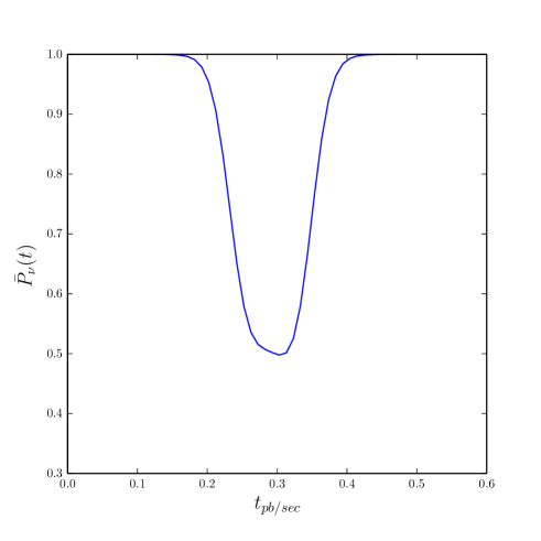
Figure 1: The approximated time-dependent survival probability $\bar{P}_{\nu\nu}(t)$ for case (b).

Recent simulations suggest quite diverse features for the details of the collective effects. In Table I, we summarize the possible scenarios resulting from the collective effects under both the normal (NH) and the inverted (IH) hierarchies, where $P_{\nu}$ and $\bar{P}_{\nu}$ represent the survival probabilities of the original $\nu_{e}$ and $\bar{\nu}_{e}$ fluxes, respectively, after the adjustment of the $\nu\nu$ self-induced collective effects. There are four different scenarios. Under NH, both $\nu_{e}$ and $\bar{\nu}_{e}$ spectra remain unaltered, i.e., $P_{\nu}\simeq 1$ and $\bar{P}_{\nu}\simeq 1$. This corresponds to case (a). The IH leads to cases (b), (c), and (d), in which the conversion probability for the $\nu_{e}$ flux can be approximated by the same step-like function of energy: $P_{s}\simeq 1$ for $E<E_{c}$, and $P_{s}\simeq 0$ for $E>E_{c}$, where $E_{c}\simeq 8$ MeV is the critical energy Fogli:2008pt . The three later cases differ in the expected $\bar{\nu}_{e}$ flux. Case (b) represents partial matter suppression of the collective effect, and the survival probability is time dependent: $\bar{P}_{\nu}=\bar{P}_{\nu}(t)$ Chakraborty:2011gd ; Chakraborty:2011nf ; Sarikas:2011am . Case (c) represents a total swap of the spectra $\bar{\nu}_{e}\leftrightarrow\bar{\nu}_{x}$: $\bar{P}_{\nu}\simeq 0$. In this case, the self-induced effect dominates over the MSW effect, see, e.g., Ref. Duan:2010bg . We add in our analysis the case (d), which indicates a complete matter suppression of the collective effect: $\bar{P}_{\nu}\simeq 1$. This corresponds to the traditional treatment of the SN $\nu$ flux based on the pure MSW effect, see, e.g., Ref. Dighe:1999bi . Note that in our calculation for scenario (b), we adopt an approximate probability function $\bar{P}_{\nu}(t)$ (as shown in Fig.1), which is fitted by the results of Ref. Chakraborty:2011gd .

Formulating the neutrino fluxes at different stages is straightforward. The primary neutrino fluxes are denoted by $F_{e}^{0}$, $F_{x}^{0}$, $\bar{F}_{e}^{0}$, and $\bar{F}_{x}^{0}$. The first modification to the $\nu$ fluxes in the SN comes from the collective effect, and the fluxes become

$$F^{c}_{e}=F^{0}_{e}+(1-P_{\nu})(F^{0}_{x}-F^{0}_{e}),$$ (2)

$$F^{c}_{x}=(1-P_{\nu})F^{0}_{e}+(1+P_{\nu})F^{0}_{x},$$ (3)

$$\bar{F}^{c}_{e}=\bar{F}_{e}^{0}+(1-\bar{P}_{\nu})(\bar{F}^{0}_{x}-\bar{F}^{0}_{e}),$$ (4)

$$\bar{F}^{c}_{x}=(1-\bar{P}_{\nu})\bar{F}^{0}_{e}+(1+\bar{P}_{\nu})\bar{F}^{0}_{x}.$$ (5)

Note that $P_{\nu}$ and $\bar{P}_{\nu}$ are given by Table I for varied scenarios and mass hierarchies.

As the neutrinos continue to propagate outwards, they encounter a further modification by the MSW effect in the SN. If one denotes the survival probability for $\nu_{e}$ ($\bar{\nu}_{e}$) after the MSW effect as $P_{m}$ ($\bar{P}_{m}$), then the fluxes of $\nu_{e}$ and $\bar{\nu}_{e}$ arriving at Earth can be written as

$$F_{e}=P_{m}F^{c}_{e}+(1-P_{m})F^{c}_{x},$$ (6)

$$\bar{F}_{e}=\bar{P}_{m}\bar{F}^{c}_{e}+(1-\bar{P}_{m})\bar{F}^{c}_{x},$$ (7)

with

$$P_{m}=|U_{e1}|^{2}P_{H}P_{L}+|U_{e2}|^{2}(P_{H}-P_{H}P_{L})+|U_{e3}|^{2}(1-P_{H}),$$ (8)

$$\bar{P}_{m}=|U_{e1}|^{2}(1-\bar{P}_{L})+|U_{e2}|^{2}\bar{P}_{L},$$ (9)

for the normal hierarchy, and

$$P_{m}=|U_{e1}|^{2}P_{L}+|U_{e2}|^{2}(1-P_{L}),$$ (10)

$$\bar{P}_{m}=|U_{e1}|^{2}\bar{P}_{H}(1-\bar{P}_{L})+|U_{e2}|^{2}\bar{P}_{H}\bar{P}_{L}+|U_{e3}|^{2}(1-\bar{P}_{H}),$$ (11)

for the inverted hierarchy. Here, $P_{H}$ and $P_{L}$ are the crossing probabilities for the neutrino eigenstates at higher and lower resonances, respectively, and the quantity with a bar represents that for $\bar{\nu}$.

After propagating through the Earth matter, the expected $\nu$ fluxes at the detectors then follow. It should be pointed out that, as compared to the analysis of Ref. Dighe:1999bi , we further consider in this work the collective effect which occurs prior to the MSW effect in the SN. Thus, in deriving the related formulation we may simply replace $F_{e}^{0}$, $F_{\bar{e}}^{0}$, $F_{x}^{0}$, and $F_{\bar{x}}^{0}$ in Ref. Dighe:1999bi by $F_{e}^{c}$, $\bar{F}_{e}^{c}$, $F_{x}^{c}$, and $\bar{F}_{x}^{c}$ of this work, respectively. We list the results here and outline the derivations in Appendix A. For the $\nu_{e}$ flux, we have

$$F^{D}_{e}\simeq F^{0}_{e}[(1-|U_{e3}|^{2})-P_{\nu}(1-2|U_{e3}|^{2})]+F^{0}_{x}[1+P_{\nu}(1-2|U_{e3}|^{2})],$$ (12)

under the normal hierarchy, and

$$F^{D}_{e}\simeq F^{0}_{e}[(1-P_{2e})-P_{\nu}(1-2P_{2e})]+F^{0}_{x}[1+P_{\nu}(1-2P_{2e})],$$ (13)

under the inverted hierarchy. As for the $\bar{\nu}_{e}$ flux, we get

$$\bar{F}^{D}_{e}\simeq\bar{F}^{0}_{e}[(1-\bar{P}_{1e})-\bar{P}_{\nu}(1-2\bar{P}_{1e})]+\bar{F}^{0}_{x}[1+\bar{P}_{\nu}(1-2\bar{P}_{1e})],$$ (14)

for the normal hierarchy, and

$$\bar{F}^{D}_{e}\simeq\bar{F}^{0}_{e}(1-\bar{P}_{\nu})+\bar{F}^{0}_{x}(1+\bar{P}_{\nu}),$$ (15)

for the inverted hierarchy. Here $P_{ie}$ ($\bar{P}_{ie}$) is the probability that a mass eigenstate $\nu_{i}(\bar{\nu}_{i}$) is observed as a $\nu_{e}$ ($\bar{\nu}_{e}$) at the detector. Note that we have used the approximation: $P_{3e}-|U_{e3}|^{2}\leq 10^{-3}$ Dighe:1999bi in writing the detected $\nu$ flux. Furthermore, we have set vanishing crossing probabilities in writing the above expressions: $P_{H}\simeq\bar{P}_{H}\simeq P_{L}\simeq\bar{P}_{L}\simeq 0$. In contrast to the matter density profile with $\rho\sim r^{-3}$ in the traditional treatment, it has been pointed out Chiu:2008sa that a local deviation of the uncertain density profile from $\rho\sim r^{-3}$ may lead to significant change of the MSW crossing probabilities for a certain range of $\theta_{13}$. This factor has been taken into consideration in our analysis. With the recent determination of the relatively large $\theta_{13}$, we conclude that the vanishing crossing probabilities can be adopted even if the local density profiles near the resonance become as steep as $\rho\sim r^{-8}$.

The probability $P_{2e}$ is usually written as $P_{2e}=\sin^{2}\theta_{12}+f_{reg}$ , with $f_{reg}$ the regeneration factor due to the Earth matter effect deHolanda:2004fd :

$$f_{reg}=\frac{2E\sin^{2}2\theta}{\delta m^{2}_{21}}\sin\Phi_{0}\sum_{i=0}^{n-1}\Delta V_{i}\sin\Phi_{i},$$ (16)

where $n$ is the number of layers, $\Delta V_{i}\equiv V_{i+1}-V_{i}$ is the potential difference between adjacent layers of matter, and $\Phi_{i}$ is the phase acquired along the trajectories. For illustrative purposes, we adopt a simple two-layer model Freund:1999vc for the Earth matter, $\rho_{E}=5.0\mbox{g/cm}^{3}$ for $R_{\oplus}/2<r<R_{\oplus}$ (mantle) and $\rho_{E}=12.0\mbox{g/cm}^{3}$ for $r<R_{\oplus}/2$ (core). Note that this two-layer analysis can be easily generalized to the analysis of a multi-layer model. The regeneration factor for two layers takes the form,

$$f_{reg}=\sin^{2}2\theta\sin\Phi_{0}[\epsilon_{m}\sin\Phi_{0}+(\epsilon_{c}-\epsilon_{m})\sin\Phi_{1}],$$ (17)

with $\epsilon_{m}=2EV_{m}/\delta m^{2}_{21}$ for the mantle and $\epsilon_{c}=2EV_{c}/\delta m^{2}_{21}$ for the core, and

$$\Phi_{0}=\frac{\delta m^{2}L}{4E}\sqrt{(\cos 2\theta-\epsilon_{m})^{2}+\sin^{2}2\theta},$$ (18)

$$\Phi_{1}=\frac{\delta m^{2}L_{1}}{4E}\sqrt{(\cos 2\theta-\epsilon_{c})^{2}+\sin^{2}2\theta}.$$ (19)

Here $L$ is the total path length inside Earth and $L_{1}$ is that inside the core.

IV Physical observables in the detectors

During the accretion phase, the detailed time evolution of the neutrino fluxes is, in general, model dependent. In this section we first adopt the ${\nu}$ and $\bar{\nu}$ fluxes during the early phase of a $10.8M_{\odot}$ progenitor SN model, such as in Ref.Chakraborty:2011nf where the flux evolution during the accretion phase was given up to 0.6s after the core bounce. We shall later discuss the possible impacts due to different choices of SN models.

For our purpose of analyzing the time structure of the energy-integrated fluxes,

$$\bar{N}(t) \sim \int\bar{F}^{D}_{e}(E,t)\cdot\bar{\sigma}_{\nu}(E)\cdot\bar{\varepsilon}(E)dE,$$

$$N(t) \sim \int F^{D}_{e}(E,t)\cdot\sigma_{\nu}(E)\cdot\varepsilon(E)dE,$$ (20)

we approximate the time-dependent number flux in Eq.(1) as piecewise functions (with arbitrary scales) based on Fig. 1 of Ref.Chakraborty:2011nf . Note that since only the flux trend around the accretion phase is relevant to our study, we omit the early flux details prior to $t_{pb}\sim 0.06$s. The fitted curves are

$$\phi_{\nu_{e}}=\left\{\begin{array}[]{ll}2.52\exp[\frac{-(t-0.13)^{2}}{0.065}],&(0<t\leq 0.25s)\\ 1.86+\exp[42.95t-13.30],&(0.25s<t\leq 0.30s)\\ 0.35+\exp[-16.65t+5.73],&(0.30s<t\leq 0.60s)\end{array}\right.$$ (21)

$$\phi_{\bar{\nu}_{e}}=\left\{\begin{array}[]{ll}1.99\exp[\frac{-(t-0.15)^{2}}{0.051}],&(0<t\leq 0.25s)\\ 1.54+\exp[35.74t-11.42],&(0.25s<t\leq 0.30s)\\ 0.35+\exp[-16.24t+5.45],&(0.30s<t\leq 0.60s)\end{array}\right.$$

$$\phi_{\nu_{x}}=\phi_{\bar{\nu}_{x}}=0.13+\exp[-3.46t+0.037], (0<t\leq 0.60s).$$ (22)

As a comparison for the qualitative features, we show in Fig.2 both the fitted curves, Eqs.(21-23), and the data points taken from the referential curves.

We assume a unity efficiency function, $\bar{\varepsilon}(E)\sim\varepsilon(E)\sim 1$, and that the limited energy resolution of the detectors is capable of observing the qualitative time evolution of the $\nu$ fluxes. The cross-section functions, $\bar{\sigma}_{\nu}(E)$ and $\sigma_{\nu}(E)$, will be presented later for each of the reaction channels. One may then check the qualitative behavior of the time structures that are the direct consequences of the mass hierarchies and distinct scenarios of the self-induced effects, as will be discussed in the following subsections.

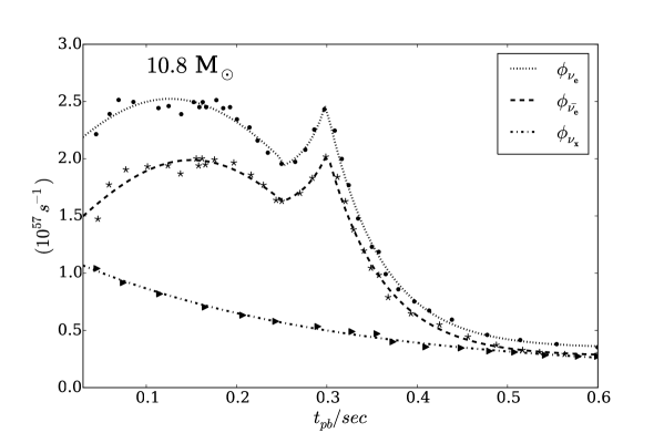
Figure 2: The curves representing Eqs.(21-23) for a $10.8M_{\odot}$ model are compared with the data points taken from the referential curves.

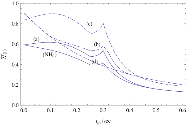
Figure 3: An estimation of $\bar{N}(t)$ (with arbitrary normalization scale) at WC or SC during the accretion phase for a $10.8M_{\odot}$ model. The four scenarios, (a), (b), (c), and (d) are resulted from different mass hierarchies and time structures of the neutrino fluxes, as listed in Table I. We have used $9\pi/10$ as the zenith angle at the detector. Note that a hypothetical scenario labeled by NH₀ is added as a reference. Note also that the outcomes for the normal hierarchy are represented by the solid lines, while that for the inverted hierarchy are represented by the dashed lines.

IV.1 $\bar{\nu}_{e}$ events at WC or SC

The inverse $\beta$ decay, $\bar{\nu}_{e}+p\rightarrow n+e^{+}$, dominates over other reaction channels in the water Cherenkov detectors and the scintillation detectors. We adopt the cross section Cadonati:2000kq : $\sigma(\bar{\nu}_{e}p)\simeq 9.5\times 10^{-44}(E-1.29)^{2}\mbox{cm}^{2}$, and assume that events originating from this channel can be properly identified. The time evolution curves of $\bar{N}(t)$ under the four possible scenarios in Table I and a hypothetical scenario (NH₀) are shown in Fig.3, and summarized as follows.

(i) A unique, monotonically decreasing $\bar{N}(t)$, which represents case (d) in Table I, is easily singled out. Observation of this result not only suggests inverted hierarchy, but also a near total suppression of the collective effect: $\bar{P}_{\nu}\simeq 1$. This result favors the scenario that MSW effect $\gg$ collective effect, which is just the traditional treatment based on the pure MSW effect without the collective effect.

(ii) An early decreasing $\bar{N}(t)$ could also arise from the time-varying survival probability $\bar{P}_{\nu}(t)$ as in case (b), which is due to partial suppression of the collective effect under the inverted hierarchy. However, a significant peak at $t_{pb}\sim 0.3s$ distinguishes this scenario from that of case (d).

(iii)A slight increase of $\bar{N}(t)$ prior to $t_{pb}\sim 0.1s$ could represent two different scenarios: normal hierarchy with $\bar{P}_{\nu}\simeq 1$ (complete suppression of the collective effect, case (a)), or inverted hierarchy with $\bar{P}_{\nu}\simeq 0$ (total spectrum swap, case (c)). Although in general the event rates could differ by roughly 50% according to a quick estimation, a definite separation between these two scenarios may not be easy if one practically considers the model uncertainties and limitations of the experimental resolution. We therefore will not stress the significance of this case here. However, further hints may be available from the observation of the $\nu_{e}$ events.

(iv) Since the overall knowledge of the oscillation effects for SN neutrinos is still insufficient, we add in Fig.3 a hypothetical case NH${}_{0}\equiv$ (NH,$\bar{P}_{\nu}\simeq 0$), even though current models in the literature do not favor this scenario. Note that, as indicated by Table I, the three scenarios (NH,$\bar{P}_{\nu}\simeq 1$), (IH,$\bar{P}_{\nu}\simeq 0$), and (IH,$\bar{P}_{\nu}\simeq 1$) are represented by cases (a), (c), and (d), respectively.

The general properties of Fig.3 can be understood as follows:

• For cases (a), (b), and (c), the peak at $t_{pb}\sim 0.3$s signals the onset of explosion. The sharp drop of $\bar{N}(t)$ and the luminosity afterwards is due to the sudden flip of matter velocities from infall to expansion when the explosion shock passes through a co-moving frame of reference where the observables are measured Chakraborty:2011gd .

• With the vanishing $\bar{P}_{H}$ and $\bar{P}_{L}$, the expected $\bar{\nu}_{e}$ flux at the detector simply inherits the shape of the $\bar{\nu}_{x}$ flux after the modification of the collective effect but before that of the MSW effect: $\bar{F}^{c}_{x}$. Eq. (5) suggests that $\bar{F}^{c}_{x}$ is a combination of $\bar{F}^{0}_{e}$ and $\bar{F}^{0}_{x}$, and the weight of each component is determined by $1-\bar{P}_{\nu}$ and $1+\bar{P}_{\nu}$, respectively. This leads to curve (d) in Fig.3 when $\bar{P}_{\nu}\simeq 1$, which corresponds to the situation when the collective effect is turned off and only the pure MSW effect is in action. In this case, the expected $\bar{F}^{0}_{e}$ simply follows the monotonically decreasing shape of $\bar{F}^{0}_{x}$ that is common in different SN models.

• As $\bar{P}_{\nu}$ decreases from $\bar{P}_{\nu}=1$, it represents the situation when the flavor transition due to the collective effect becomes more important, and the fraction of $\bar{F}^{0}_{e}$ becomes larger. The direct consequence is that the shape of $\bar{F}^{0}_{e}$ becomes more prominent and thus the peak, which is the characteristic feature of $\bar{F}^{0}_{e}$, begins to emerge as in cases (b) and (c) under the inverted hierarchy.

• The shape of case (a) under the normal hierarchy can be understood by the same reasoning. With $\bar{P}_{L}\sim 0$, Eqs.(7) and (9) suggest that $\bar{F}_{e}\simeq|U_{e1}|^{2}\bar{F}^{c}_{e}+(1-|U_{e1}|^{2})\bar{F}^{c}_{x}$, i.e., $\bar{F}_{e}$ is a superposition of $\bar{F}^{c}_{e}$ and $\bar{F}^{c}_{x}$, with the fractions of $|U_{e1}|^{2}$ and $1-|U_{e1}|^{2}$, respectively. This results in the appearance of the characteristic peak at $t_{pb}\sim 0.3$s, but not as prominently as in cases (b) and (c).

• At the early stage, (b) and (d) are indistinguishable since $\bar{P}_{\nu}\simeq 1$ for case (d), while the time-varying probability for case (b) also remains at $\bar{P}_{\nu}\simeq 1$ before it drops to $\sim 1/2$ (when the complete flavor mixture occurs Chakraborty:2011nf ) near $t_{pb}\sim 0.3$s.

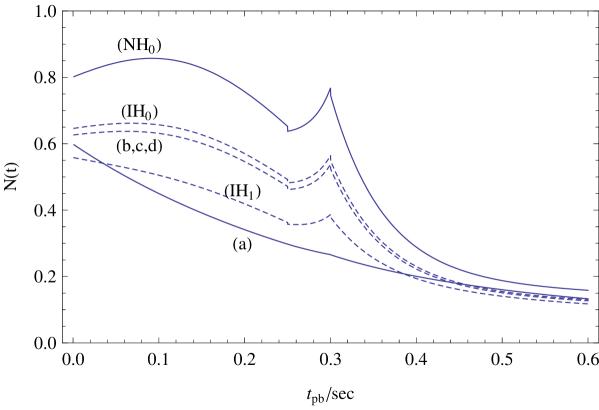
Figure 4: An estimation of $N(t)$ (with arbitrary normalization scale) at the Ar detector during the accretion phase for a $10.8M_{\odot}$. We have used $9\pi/10$ as the zenith angle at the detector. Note that the outcomes for the normal hierarchy are represented by the solid lines, while that for the inverted hierarchy are represented by the dashed lines.

IV.2 $\nu_{e}$ events at liquid Ar detectors

The cross section for the charged-current reaction, $\nu_{e}+^{40}Ar\rightarrow^{40}K^{*}+e^{-}$, is given by Cocco:2004ac $\sigma(\nu_{e}Ar)\simeq 3.38\times 10^{-42}(E_{\nu}/\mbox{MeV})\mbox{cm}^{2}$. We show in Fig.4 the expected time-varying behavior for the dominant $\nu_{e}$-induced events at the Ar detector. It is clearly seen that the case under NH with $P_{\nu}\simeq 1$ (case (a)) leads to monotonically decreasing rates, while a significant bump near $t_{pb}\sim 0.3s$ appears for IH with $P_{\nu}\simeq P_{s}$ for cases (b), (c), and (d). These totally distinct time structures lift the degeneracy of the $\bar{\nu}_{e}$ result between (a) and (c) for case (iii) in the previous subsection, and can act as a supplement to the observation of the $\bar{\nu}_{e}$ flux. Note that one may also reason the properties of the curves in Fig.4 by examining the details of Eq. (6). In addition, three hypothetical scenarios are shown in Fig.4 as a reference, with NH${}_{0}\equiv$ (NH,$P_{\nu}=0$), IH${}_{0}\equiv$ (IH,$P_{\nu}=0$), and IH${}_{1}\equiv$ (IH,$P_{\nu}=1$). So far, these three scenarios are not favored by current models in the literature.

IV.3 Analysis with varying incident angles

The angle of incidence at the detector is arbitrary for the SN $\nu$ fluxes, although preferred detector locations were predicted-see, e.g., Ref.Mirizzi:2006xx . A zenith angle $9\pi/10$ (mantle +core) has been adopted in our calculation. To investigate the possible deviation from our analysis, we also show the results for $3\pi/5$ (mantle) and $0.01\pi$ ($\sim$ no Earth matter) in Fig.5. With the varying depth of the path into the Earth, the Earth effect will in principle, modify the fluxes accordingly, as indicated by the wiggles. The observability of the Earth effect has been discussed elsewhere, see, e.g., Ref.Borriello:2012zc ; Choubey:2010up . Fig.5 suggests that the angle of incidence for the $\nu$ fluxes may modify the details of the observed fluxes, but not the qualitative trend of the spectra. In our analysis, we study the general time evolution of the expected fluxes, regardless of whether or not the detailed Earth effect can be observed.

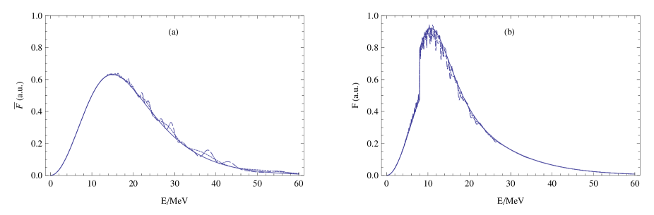
Figure 5: The expected $\bar{\nu}_{e}$ flux at the WC or SC detectors for case (a), and the $\nu_{e}$ flux arriving at the Ar detector for case (b). Three different zenith angles at the detectors are adopted: $0.01\pi$ (solid), $3\pi/5$ (dotted), and $9\pi/10$ (dashed). Despite the slight wiggles due to the Earth effect, the general trend of the curves is unaltered. Note that the curves are plotted with arbitrary scales.

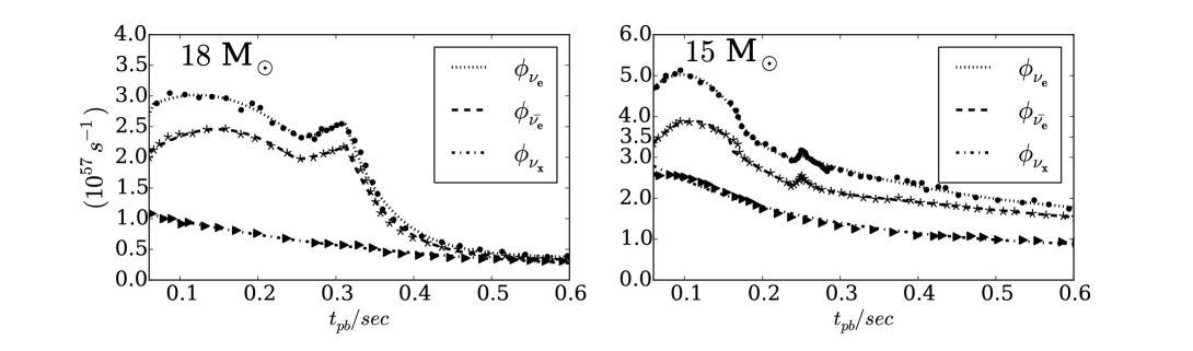
Figure 6: The curves representing Eqs.(21-23) for a $18M_{\odot}$ and a $15M_{\odot}$ models are compared with the data points taken from the referential curves.

IV.4 Analysis with varying models

In the previous analysis, we have adopted a specific, $10.8M_{\odot}$ Fe-core progenitor model. The time structure of the $\nu$ flux, which is model dependent, has been the main focus of the study. To examine the general futures and the trend of the $\nu$ luminosity obtained from other models, we further fit the neutrino number flux for $18M_{\odot}$ Fischer:2009af and $15M_{\odot}$ models Borriello:2012zc Fischer:2009af . For the $18M_{\odot}$ model, we have

$$\phi_{\nu_{e}}=\left\{\begin{array}[]{ll}2.52\exp[\frac{-(t-0.13)^{2}}{0.065}],&(0<t\leq 0.25s)\\ 1.86+\exp[42.95t-13.30],&(0.25s<t\leq 0.30s)\\ 0.35+\exp[-16.65t+5.73],&(0.30s<t\leq 0.60s)\end{array}\right.$$ (23)

$$\phi_{\bar{\nu}_{e}}=\left\{\begin{array}[]{ll}1.99\exp[\frac{-(t-0.15)^{2}}{0.051}],&(0<t\leq 0.25s)\\ 1.54+\exp[35.74t-11.42],&(0.25s<t\leq 0.30s)\\ 0.35+\exp[-16.24t+5.45],&(0.30s<t\leq 0.60s)\end{array}\right.$$

$$\phi_{\nu_{x}}=\phi_{\bar{\nu}_{x}}=0.13+\exp[-3.46t+0.037], (0<t\leq 0.60s),$$ (24)

and the $15M_{\odot}$ model leads to

$$\phi_{\nu_{e}}=\left\{\begin{array}[]{ll}5.025\exp[\frac{-(t-0.098)^{2}}{0.023}],&(0.06s<t\leq 0.16s)\\ 2.78+\exp[-25.19t+4.38],&(0.16s<t\leq 0.227s)\\ 2.91+\exp[39.58t-10.87],&(0.227s<t\leq 0.253s)\\ 1.66+\exp[-3.76t+1.47],&(0.253s<t\leq 0.6s)\end{array}\right.$$

$$\phi_{\bar{\nu}_{e}}=\left\{\begin{array}[]{ll}3.89\exp[\frac{-(t-0.098)^{2}}{0.018}],&(0.06s<t\leq 0.177s)\\ 0.079+\exp[-4.10t+1.79],&(0.177s<t\leq 0.24s)\\ 2.22+\exp[106.76t-27.85],&(0.24s<t\leq 0.25s)\\ 2.12+\exp[-60.33t+14.26],&(0.25s<t\leq 0.30s)\\ -0.78+\exp[-0.74t+1.29],&(0.30s<t\leq 0.6s)\end{array}\right.$$

$$\phi_{\nu_{x}}=\phi_{\bar{\nu}_{x}}=0.71+\exp[-4.62t+1.01], (0.06s<t\leq 0.6s).$$ (25)

In Fig.6, we show the fitted curves and the data points taken from the referential curves for both the $18M_{\odot}$ and $15M_{\odot}$ models.

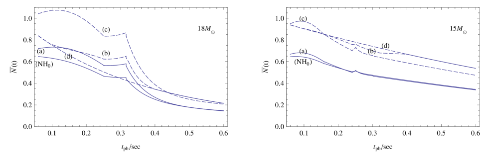
Figure 7: The resultant $\bar{N}(t)$ from a $18M_{\odot}$ and a $15M_{\odot}$ models.

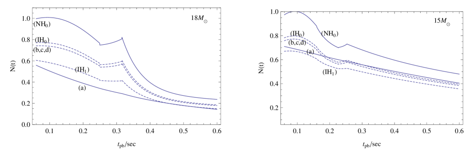
Figure 8: The resultant $N(t)$ from a $18M_{\odot}$ and a $15M_{\odot}$ models.

The resultant $\bar{N}(t)$ and $N(t)$ from Eq.(20) are shown in Figs.7 and 8, respectively. One may compare Fig.3 with Fig.7 for $\bar{N}(t)$, and Fig.4 with Fig.8 for $N(t)$. Note that for the $15M_{\odot}$ model, the peaks of both $\bar{N}(t)$ and $N(t)$ occur near $t_{pb}\sim 0.25$s and are less prominent as compared to other models. It can be seen that the expected neutrino events derived from models of different SN masses do share certain qualitative features that may be applied to the study of neutrino properties, as outlined in the previous subsections. However, one should also keep in mind that for complex physical processes such as SN events, a large portion of our knowledge from various models in the literature still remains uncertain. The characteristic distinctions among models make the analysis of SN neutrinos challenging, and more detailed models and analysis are definitely in high demand. In fact, we should point out that along the line of our analysis, it is difficult, if not impossible, to apply our arguments to the results of, e.g., the $8.8M_{\odot}$ model Fischer:2009af , as shown in Fig.9. Nevertheless, a qualitative analysis based on certain types of models such as the one discussed in this paper might be considered as one of the preliminary and alternative approaches that could pave the way for future study.

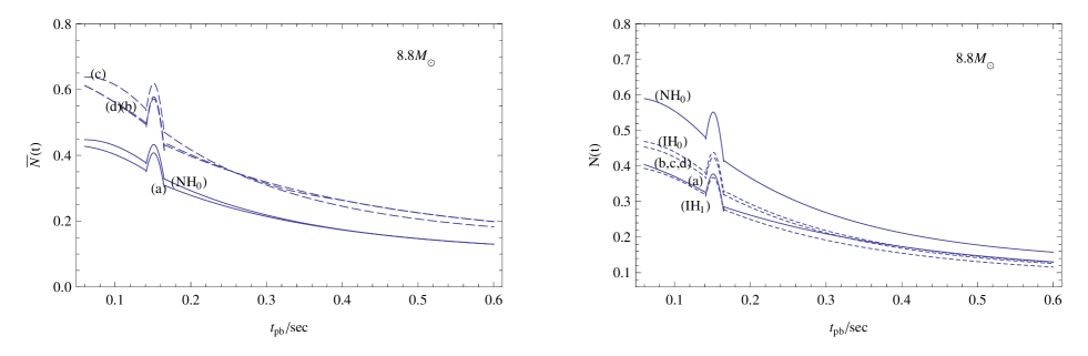
Figure 9: The resultant $\bar{N}(t)$ and $N(t)$ from a $8.8M_{\odot}$ model.

V Conclusion

The multi-angle analysis of SN neutrinos in the collective oscillations suggests that the dense matter during the early, accretion phase may suppress the self-induced flavor conversion and lead to time-dependent transition probabilities. Investigation of the neutrino signals that are modified by the influence of various collective effects, in addition to the usual MSW and the Earth matter effects, may shed light on the undetermined neutrino mass hierarchy. On the other hand, the time structures of the collective flavor conversion resulting from the model uncertainties and the neutrino mass hierarchies during the accretion phase may also leave signatures on the observed $\nu_{e}$ and $\bar{\nu}_{e}$ fluxes.

Intense effort has been devoted to the general study of SN neutrino flavor conversion. Related topics, such as probing the neutrino parameters or analyzing the detectability of varied effects on the SN neutrinos, have also been widely discussed. To better clarify our motivation in this work and to distinguish our work from others, we briefly outline here the aims of similar studies in the literature:

• In Choubey et al. Choubey:2010up , the expected neutrino signals resulting from varied flux models were calculated and the signatures, especially the patterns of spectral split, of the collective effects are examined. The flavor conversion during the accretion phase was also discussed. However, the possibility that very dense ordinary matter may suppress the collective conversion during the accretion phase, a consequence of the multi-angle analysis, was not included. The related discussion thus corresponds to distinguishing case (a) for the NH and case (c) for the IH in our paper.

• The paper by Borriello et al. Borriello:2012zc aimed at the observability of the Earth matter effect for SN neutrinos. The time-integrated spectra during part of the accretion phase and the cooling phase were taken as benchmarks for the calculation. For flavor conversion, the complete matter suppression of the collective effect was considered, and the neutrinos underwent only the dominant MSW conversion in the SN. The related discussions correspond to separating case (a) and case (d) in our analysis.

• In Serpico et al. Serpico:2011ir , the analysis was focused on probing the neutrino mass hierarchy with the neutrino signals at the IceCube Cherenkov detector. Complete matter suppression of the collective effect during the early era of the accretion phase ($t_{pb}<0.2s$) was considered. In this analysis the MSW conversion also plays the dominant role. The related discussion thus corresponds to distinguishing case (a) and case (d) as in part of our analysis ($t_{pb}<0.2s$), but based on the outcome of a different detector.

Our approach differs from the above analyses mainly in that, as far as the influence of the collective effect is considered, we focus on the time-varying collective flavor conversion probability and the resultant time-dependent neutrino fluxes during the accretion phase, up to $t_{pb}\sim 0.6s$. Thus, the possible consequences due to (i) a complete suppression of the collective effect, (ii) a partial suppression of the collective effect, and (iii) a large collective effect are all discussed. Given the current situation that uncertainty still remains in the mechanism of the collective effect, our discussion covers the scope that allows model uncertainties in the time structures of the flavor conversion and the fluxes. Furthermore, our analysis was established based on a conservative assumption that the Earth matter effect is beyond detectable. More precisely, observing a specific effect, such as the collective effect or the Earth matter effect, is not the main issue in our paper and is irrelevant to our aim, although it could be crucial to other analyses. In fact, it was suggested Borriello:2012zc that observing the Earth effect under a general situation may be more challenging than expected, and the optimistic view toward an identification of the neutrino mass hierarchy may need to be re-evaluated. In a sense, this may also suggest that one should try to avoid as many as possible the factors that may complicate the interpretation of the signals in probing the neutrino mass hierarchy. Regardless of the observability of the Earth matter effect, our analysis seems in agreement with this logic by establishing the qualitative properties that are unaffected by whether or not the Earth matter effect can be singled out.

It should be pointed out that the details of the time structure for the primary $\nu$ fluxes and their relative magnitude are, of course, model dependent. However, the general qualitative features do not vary much among the analyzed models, as discussed in Sec. IV. As far as our purposes are concerned, the qualitative study should be able to provide moderate hints as an addition to those of the numerical studies that may suffer from model uncertainties and the experimental details involved. In addition, out of the three independent effects included in our calculation, the time-dependent collective effect plays a key role in our analysis because the variation of the expected outcome is determined almost entirely by the not-so-well understood collective effect. In this regard, we further analyze the time structure of the consequences resulting from different models. The results may also help shed light on identifying the working scenario of the collective effect in supernovae.

We have assumed equipartitioned luminosity for the neutrino flavors, as mentioned in Section II. Note that the relative magnitude of the luminosity may not remain the same during the later cooling phase. Even in the case of a slight deviation from the equipartition during the accretion phase, our qualitative analysis, which focuses on the trend of event rate in time, remains valid since the numerical details involved in the calculation do not alter the general pictures of the physical observables.

Our results suggest that not only the mass hierarchy, but also the SN mechanism related to the collective effect may, in principle, be resolved to certain extent by the observation of both $\nu$ and $\bar{\nu}_{e}$ fluxes. However, this physics potential of observing SN neutrinos relies heavily on the resolution power of a detector and proper numerical analysis. A more detailed numerical study, which takes into consideration the possible consequences due to different models, variation of the luminosity strength, and the experimental details, would certainly be in high demand and shall be discussed elsewhere. In this work, we only estimate the qualitative properties of the observables. Nevertheless, it is still hoped that analysis along this line would provide an alternative approach toward a better understanding of SN neutrinos, especially under the current situation that the model uncertainties exist and a comprehensive knowledge of SN physics is still lacking.

Appendix A Derivation of $\nu$ fluxes at the detector

We briefly summarize the derivations of Eqs.(12-15) here. Note, as mentioned in the text, that we have imposed the approximate conditions $P_{3e}-|U_{e3}|^{2}\leq 10^{-3}$ and $P_{H}\simeq\bar{P}_{H}\simeq P_{L}\simeq\bar{P}_{L}\simeq 0$ in writing Eqs.(12-15) from part of the following derivations.

The original fluxes $F_{e}^{0}$ and $F_{x}^{0}$ in Eq.(69) of Ref.Dighe:1999bi ,

$$F^{D}_{e}\simeq F_{e}+P_{H}(P_{2e}-|U_{e2}|^{2})(1-2P_{L})(F_{e}^{0}-F_{x}^{0}),$$ (26)

should be respectively replaced by our $F_{e}^{c}$ (Eq.(2)) and $F_{x}^{c}$ (Eq.(3)) to account for the collective effect:

$$F^{D}_{e}\simeq F_{e}+P_{H}(P_{2e}-|U_{e2}|^{2})(1-2P_{L})(F_{e}^{c}-F_{x}^{c}),$$ (27)

where $F_{e}$, as given by Eq.(6), is the $\nu_{e}$ flux arriving at Earth. Eq. (27) leads directly to $F_{e}^{D}$ under the normal hierarchy, as given by Eq.(12), if one imposes the approximate conditions.

In addition, since the conversion of $\nu_{e}$ is independent of $P_{H}$ under the inverted hierarchy, we may simply set $P_{H}=1$ in Eq.(71) of Ref.Dighe:1999bi and use their Eq.(69) to obtain the expression for $F_{e}^{D}$ under the inverted hierarchy. This leads to Eq.(13) if one again replaces $F_{e}^{0}-F_{x}^{0}$ by $F_{e}^{c}-F_{x}^{c}$.

As for the $\bar{\nu}_{e}$ flux at the detector under the normal hierarchy, we use Eq.(79) of Ref.Dighe:1999bi and replace $F_{\bar{e}}^{0}$ and $F_{x}^{0}(=F_{\bar{x}}^{0})$ respectively by $\bar{F}_{e}^{c}$ (Eq.(4)) and $\bar{F}_{x}^{c}$ (Eq.(5)). This leads to the expression of $\bar{F}_{e}^{D}$ in Eq.(14). Note that the original flux of $\nu_{x}$ is usually set to be identical to that of $\bar{\nu}_{x}$, $F_{x}^{0}=F_{\bar{x}}^{0}$.

Finally, for the inverted hierarchy, the $\bar{\nu}_{e}$ spectrum is the same as the normal one except for a suppression factor $\bar{P}_{H}$. In this case, $\bar{F}_{e}^{D}$ in Eq.(15) can be derived from Eq.(106) of Ref.Dighe:1999bi by setting $D_{2}$ at the location where the $\nu$ flux enters the Earth so that $F_{\bar{e}}^{D2}=\bar{F}_{e}$ and $\bar{P}_{1e}^{(2)}=|U_{e1}|^{2}$. Explicitly, one may refer to, e.g., Eq.(27) of Ref. Lunardini:2001pb . Following this line, one reaches Eq.(15) if $F_{\bar{e}}^{0}-F_{x}^{0}$ there in Ref.Dighe:1999bi or Lunardini:2001pb is replaced by $\bar{F}_{e}^{c}-\bar{F}_{x}^{c}$.

References

- (1) J. T. Pantaleone, Phys. Lett. B 287, 128 (1992) Y. Z. Qian and G. M. Fuller, Phys. Rev. D 51, 1479 (1995) H. Duan, G. M. Fuller and Y. -Z. Qian, Phys. Rev. D 74, 123004 (2006) H. Duan, G. M. Fuller, J. Carlson and Y. -Z. Qian, Phys. Rev. D 74, 105014 (2006) S. Hannestad, G. G. Raffelt, G. Sigl and Y. Y. Y. Wong, Phys. Rev. D 74, 105010 (2006)
- (2) H. Duan, G. M. Fuller and Y. -Z. Qian, Ann. Rev. Nucl. Part. Sci. 60, 569 (2010)
- (3) L. Wolfenstein, Phys. Rev. D 17, 2369 (1978) S. P. Mikheev and A. Y. .Smirnov, Sov. J. Nucl. Phys. 42, 913 (1985) [Yad. Fiz. 42, 1441 (1985)]
- (4) G. L. Fogli, E. Lisi, A. Marrone and A. Mirizzi, JCAP 0712, 010 (2007)
- (5) B. Dasgupta, A. Dighe, G. G. Raffelt and A. Y. .Smirnov, Phys. Rev. Lett. 103, 051105 (2009)
- (6) G. G. Raffelt, Prog. Part. Nucl. Phys. 64, 393 (2010).
- (7) F. P. An et al. [DAYA-BAY Collaboration], Phys. Rev. Lett. 108, 171803 (2012)
- (8) J. K. Ahn et al. [RENO Collaboration], Phys. Rev. Lett. 108, 191802 (2012)
- (9) A. Esteban-Pretel, A. Mirizzi, S. Pastor, R. Tomas, G. G. Raffelt, P. D. Serpico and G. Sigl, Phys. Rev. D 78, 085012 (2008)
- (10) S. Chakraborty, T. Fischer, A. Mirizzi, N. Saviano and R. Tomas, Phys. Rev. D 84, 025002 (2011)
- (11) S. Chakraborty, T. Fischer, A. Mirizzi, N. Saviano and R. Tomas, Phys. Rev. Lett. 107, 151101 (2011)
- (12) S. Sarikas, G. G. Raffelt, L. Hudepohl and H. -T. Janka, Phys. Rev. Lett. 108, 061101 (2012)
- (13) J. Beringer et al. (Particle Data Group), Phys. Rev. D 86, 010001 (2012)
- (14) T. Totani, K. Sato, H. E. Dalhed and J. R. Wilson, Astrophys. J. 496, 216 (1998)
- (15) M. T. .Keil, G. G. Raffelt and H. -T. Janka, Astrophys. J. 590, 971 (2003)
- (16) P. D. Serpico, S. Chakraborty, T. Fischer, L. Hudepohl, H. -T. Janka and A. Mirizzi, Phys. Rev. D 85, 085031 (2012)
- (17) G. L. Fogli, E. Lisi, A. Marrone, A. Mirizzi and I. Tamborra, Phys. Rev. D 78, 097301 (2008)
- (18) A. S. Dighe and A. Y. Smirnov, Phys. Rev. D 62, 033007 (2000)
- (19) S. -H. Chiu and T. -K. Kuo, Phys. Rev. D 73, 033007 (2006) S. -H. Chiu, Phys. Rev. D 76, 045004 (2007) S. -H. Chiu, Mod. Phys. Lett. A 24, 2741 (2009)
- (20) P. C. de Holanda, W. Liao and A. Y. Smirnov, Nucl. Phys. B 702, 307 (2004)
- (21) M. Freund and T. Ohlsson, Mod. Phys. Lett. A 15, 867 (2000)
- (22) L. Cadonati, F. P. Calaprice and M. C. Chen, Astropart. Phys. 16, 361 (2002)
- (23) A. G. Cocco, A. Ereditato, G. Fiorillo, G. Mangano and V. Pettorino, JCAP 0412, 002 (2004)
- (24) A. Mirizzi, G. G. Raffelt and P. D. Serpico, JCAP 0605, 012 (2006)
- (25) E. Borriello, S. Chakraborty, A. Mirizzi, P. D. Serpico, and I. Tamborra, Phys. Rev. D 86, 083004 (2012)
- (26) S. Choubey, B. Dasgupta, A. Dighe and A. Mirizzi, arXiv:1008.0308 [hep-ph]
- (27) T. Fischer, S. C. Whitehouse, A. Mezzacappa, F. -K. Thielemann and M. Liebendorfer, Astron. Astrophys. 517, A80 (2010)
- (28) C. Lunardini and A. Y. Smirnov, Nucl. Phys. B 616, 307 (2001) [hep-ph/0106149].