Hyperbolicity of renormalization of circle maps with a break-type singularity

Abstract.

We study the renormalization operator of circle homeomorphisms with a break point and show that it possesses a hyperbolic horseshoe attractor.

1. Preliminaries

Renormalization of homeomorphisms of the circle with a break singularity.

This work concerns renormalization of homeomorphisms of the circle ${\mathbb{T}}={\mathbb{R}}/{\mathbb{Z}}$ with a break singularity. Specifically, these are mappings

$$f:{\mathbb{T}}\to{\mathbb{T}}$$

with the following properties:

• $f\in C^{2+\epsilon}({\mathbb{T}}\setminus\{0\})$ for some $\epsilon>0$, and $f\in C^{0}({\mathbb{T}})$;

• $f^{\prime}(x)>0$ for all $x\neq 0$;

• $f$ has one-sided derivatives $f^{\prime}(0+)>0$ and $f^{\prime}(0-)>0$ and

  $$f^{\prime}(0-)/f^{\prime}(0+)=c^{2}\neq 1.$$

Renormalizations of such maps were extensively studied by the first author and others (see e.g. [VK, KK, KT2]). We recall the definition of renormalization of a circle homeomorphism $f$ at a point $x_{0}\in{\mathbb{T}}$ (to fix the ideas we will set $x_{0}=0$) very briefly, the reader will find a detailed account in any of the above references. Firstly, let us denote $\rho(f)$ the rotation number of $f$. Denote $\bar{f}:{\mathbb{R}}\to{\mathbb{R}}$ the lift of $f$ to the real line via the projection $x\mapsto x\operatorname{mod}{\mathbb{Z}}$ with the property $\bar{f}(0)\in[0,1)$. Assume that $\rho(f)\neq 0$, and consider the smallest $r_{0}\in{\mathbb{N}}$ for which

$$1\in[\bar{f}^{r_{0}}(0),\bar{f}^{r_{0}+1}(0)).$$

Denote $I_{0}=[0,\bar{f}(0)]$, $I_{1}=[\bar{f}^{r_{0}}(0)-1,0]$ and let $\zeta_{1}:I_{0}\cup I_{1}\to I_{0}\cup I_{1}$ be the pair of interval homeomorphisms

$$\zeta_{1}=(({\bar{f}}^{r_{0}}-1)|_{I_{0}},\bar{f}|_{I_{1}}).$$

The first renormalization ${\cal R}(f)=(\eta_{1},\xi_{1})$ is the rescaled pair $\alpha_{1}\circ\zeta_{1}\circ\alpha_{1}^{-1}$ where $\alpha_{1}$ is the orientation-reversing rescaling $x\mapsto-x/\bar{f}(0).$ Thus,

$$\eta_{1}:[-1,0]\to[-b_{1},a_{1}]\text{ and }\xi_{1}:[0,a_{1}]\to[-1,-b_{1}],$$

where $-b_{1}=\alpha_{1}(\bar{f}^{r_{0}+1}(0)-1)\in[-1,0]$ and $a_{1}=\alpha_{1}(\bar{f}^{r_{0}}(0)-1)>0.$

We can now proceed to inductively define a finite or infinite sequence of renormalizations ${\cal R}^{n}(f)=(\eta_{n},\xi_{n})$ as follows. Consider the smallest $r_{n}\in{\mathbb{N}}$ such that

$$0\in[\eta_{n}^{r_{n}}(\xi(0)),\eta^{r_{n}+1}(\xi(0))).$$

We refer to $r_{n}$ as the height of $\zeta_{n}=(\eta_{n},\xi_{n})$. If such a number does not exist, then $f$ is renormalizable only $n$ times; set $r_{n}=\infty$ and terminate the sequence. Otherwise, set $\alpha_{n+1}(x)=-x/\xi_{n}(0)$ and let ${\cal R}^{n}f=(\eta_{n+1},\xi_{n+1}),$ where

$$\eta_{n+1}=\alpha_{n+1}\circ\eta_{n}^{r_{n}}\circ\xi_{n}\circ\alpha_{n+1}^{-1}:[-1,0]\to[-b_{n+1},a_{n+1}]\text{ and }$$

$$\xi_{n+1}=\alpha_{n+1}\circ\eta_{n}\circ\alpha_{n+1}^{-1}:[0,a_{n+1}]\to[-1,b_{n+1}].$$

It will also be convenient for us to introduce the $n$-th pre-renormalization

(1.1) $$p{\cal R}^{n}f\equiv(\gamma_{n}^{-1}\circ\eta_{n}\circ\gamma_{n},\gamma_{n}^{-1}\circ\xi_{n}\circ\gamma_{n}),$$

where

$$\gamma_{n}\equiv\alpha_{n}\circ\alpha_{n-1}\circ\cdots\circ\alpha_{1}.$$

Thus, $p{\cal R}^{n}f$ is a composition of iterates of the original pair $\zeta_{1}$, and ${\cal R}^{n}f$ is its suitable rescaling.

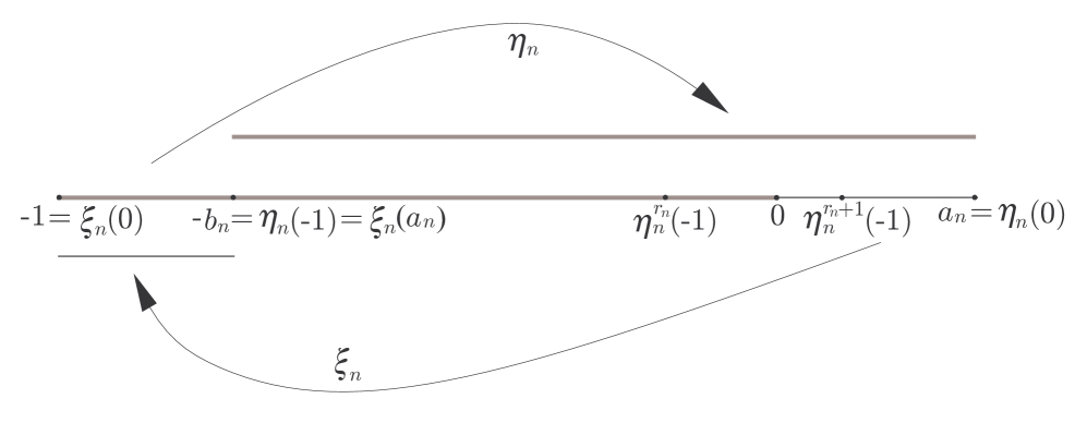
Figure 1. The dynamics of the pair $(\eta_{n},\xi_{n})$.

Using the convention $1/\infty=0$, we recover $\rho(f)$ as the finite or infinite continued fraction

$$\rho(f)=[r_{0},r_{1},r_{2},\ldots].$$

Note that one advantage of defining the continued fraction via the dynamics of $f$ as above is that we obtain a canonical expansion for all rational rotation numbers $\rho(f)$.

The invariant family of Möbius transformations.

Fix a value of $c\neq 1$, and define two families of Möbius transofrmations

$$F_{a,v,c}(z)=\frac{a+cz}{1-vz},\text{ and }G_{a,v,c}(z)=\frac{a(z-c)}{ac+z(1+v-c)}.$$

Set

$$\zeta_{a,v,c}\equiv(F_{a,v,c},G_{a,v,c}):[-1,a]\to[-1,a].$$

The parameter $c$ can be read off from

(1.2) $$c^{2}=\frac{F_{a,v,c}^{\prime}(0)G^{\prime}_{a,v,c}(F_{a,v,c}(0))}{G_{a,v,c}^{\prime}(0)F^{\prime}_{a,v,c}(-1)}.$$

Observe that

(1.3) $$-b\equiv F_{a,v,c}(-1)=G_{a,v,c}(a)=\frac{a-c}{1+v},\;F(0)=a,\;G(0)=-1.$$

We set the following additional constraints:

• $c\geq a>0$;

• $b=(c-a)/(v+1)\in[0,1)$.

Together with equalities (1.3), the above conditions imply (see Lemma 4. in [KK]):

Proposition 1.1.

The maps

$$F_{a,v,c}:[-1,0]\to[-b,a]\text{ and }G_{a,v,c}:[0,a]\to[-1,-b]$$

are orientation preserving homeomorphisms. Further,

$$F^{\prime}_{a,v,c}(z)>0\text{ for }z\in[-1,0],\text{ and }G^{\prime}_{a,v,c}(z)>0\text{ when }z\in[0,a].$$

Denote

$$\pi:{\mathbb{R}}\to{\mathbb{R}}/{\mathbb{Z}}\text{ the projection }x\mapsto x\operatorname{mod}{\mathbb{Z}},$$

and set

$$z\equiv-\frac{a}{c}=(F_{a,v,c})^{-1}(0)\in[-1,0].$$

Identifying the circle ${\mathbb{R}}/{\mathbb{Z}}$ with $[-1,0]$ via the projection $\pi$, we can view the pair of maps

$$\tau_{a,v,c}\equiv(F_{a,v,c}|_{[-1,z]},G_{a,v,c}\circ F_{a,v,c}|_{[z,0]}):[-1,0]\mapsto[-1,0]$$

as a circle homeomorphism

(1.4) $$f_{a,v,c}(z)=\pi\circ\tau_{a,v,c}\circ\pi^{-1}.$$

We will denote its rotation number

$$\rho(f_{a,v,c})\equiv\rho(\zeta_{a,v,c})=[r_{0},r_{1},\ldots].$$

In the case when $r_{0}\neq\infty$, we define the pre-renormalization

$$p{\cal R}\zeta_{a,v,c}\equiv(F_{a,v,c}^{r_{0}}\circ G_{a,v,c}|_{[0,a]},F_{a,v,c}|_{[F_{a,v,c}^{r_{0}}\circ G_{a,v,c}(0),0]}).$$

The following invariance property of the family $(F_{a,v,c},G_{a,v,c})$ is of a key importance:

Proposition 1.2.

Suppose $\rho(\zeta_{a,v,c})\neq 0$. Then the renormalization of a pair $\zeta_{a,v,c}=(F_{a,v,c}(z),G_{a,v,c}(z))$ is of the form $\zeta_{a^{\prime},v^{\prime},1/c}$ for some $a^{\prime}$, $v^{\prime}$.

Further, the following holds (see [VK, KV]):

Theorem 1.3.

Let $f$ be a circle mapping with a break singularity of class $C^{2+\epsilon}$, with break size $c$. Let $\zeta_{n}=(\eta_{n},\xi_{n})={\cal R}^{n}(f)$, and $a_{n}=\eta_{n}(0)$, $-b_{n}=\xi_{n}(0)$ as above. Set $c_{n}=c$ for $n$ even and $c_{n}=1/c$ for $n$ odd, and $v_{n}=(c_{n}-a_{n}-b_{n})/b_{n}$. Then there exist constants $C>0$ and $0<\lambda<1$ such that

$$||\eta_{n}-F_{a_{n},v_{n},c_{n}}||_{C^{2}([-1,0])}\leq C\lambda^{n}\text{ and }||\xi_{n}-G_{a_{n},v_{n},c_{n}}||_{C^{2}([0,a_{n}])}\leq C\lambda^{n}/a_{n}\text{.}$$

At this point it is instructive to draw parallels with the theory of renormalization of critical circle maps (see [Ya1, Ya2, Ya3] and references therein). The ${\cal R}$-invariant two-dimensional parameter space $(a,v)$ of pairs of Möbius maps is an analogue of the Epstein class ${\cal E}$ of critical circle maps. Similarly to Proposition 1.3, renormalizations of smooth critical circle maps converge to ${\cal E}$ geometrically fast. The maps in ${\cal E}$ are analytic and possess rigid global structure, yet the Epstein class does not embed into a finite-dimensional space. In fact, as shown in [Ya2] by the second author, suitably defined conformal conjugacy classes of maps in ${\cal E}$ form a Banach manifold. This has required developing an extensive analytic machinery to tackle renormalization convergence and hyperbolicity in ${\cal E}$ (see [Ya3], which is the culmination of this work, and references therein). In contrast, the finite dimensionality of the space $(a,v)$ allows for a direct approach to proving hyperbolicity of ${\cal R}$ restricted to this invariant space.

Note that since maps with a break singularity are only $C^{0}$ at the origin, it does not make sense to speak of renormalization of commuting pairs, the way one does for critical circle maps. We note, however, that maps $F_{a,v,c}$ and $G_{a,v,c}$ satisfy the following commutation condition:

(1.5) $$G(F(z))=F(G(c^{2}z)).$$

While one can readily check this algebraically, Theorem 1.3 leads to the same conclusion. Indeed, compare the value of the iterate $f^{q_{n}+q_{n+1}}$ to the left and to the right of zero. Since $f^{\prime}(0-)/f^{\prime}(0+)=c^{2}$, we have (in a self-explanatory notation),

$$f^{q_{n}+{q_{n+1}}}(0-)=f^{q_{n}+{q_{n+1}}}(c^{2}\cdot 0+).$$

Since the compositions $\eta_{n}\circ\xi_{n}$ and $\xi_{n}\circ\eta_{n}$ are both obtained by linearly rescaling the above iterate (on different sides of $0$), the equality (1.5) holds for limits of renormalizations.

Renormalization on the space of Möbius pairs.

Let us denote

$${\cal D}_{c}=\{(a,v)\;|\;0<a\leq c\text{ and }a+v>c-1\}.$$

The set ${\cal O}^{n}_{c}\subset{\cal D}_{c}$ consists of pairs $(a,v)$ for which the pair $\zeta_{a,v,c}=(F_{a,v,c},G_{a,v,c})$ is $n$-times renormalizable. The infinite intersection

$${\cal O}^{\infty}_{c}=\cap_{n\in{\mathbb{N}}}{\cal O}^{n}_{c}$$

is the set of infinitely renormalizable pairs. It can be equivalently characterized as the set of pairs $\zeta_{a,v,c}$ with an irrational rotation number. The set of renormalizable pairs ${\cal O}^{1}_{c}$ is naturally stratified into a collection of subsets

$$\Pi_{k,c}=\{(a,v)\text{ such that }\zeta_{a,v,c}\text{ has height }r=k\in{\mathbb{N}}\}.$$

In particular, for $(a,v)\in\Pi_{k,c}$ the rotation number $\rho(\zeta_{a,v,c})$ can be expanded into a continued fraction of the form $[k,\ldots]$.

We define the renormalization operator

$${\cal R}_{c}:{\cal O}^{1}_{c}\to{\cal D}_{1/c},$$

as $(a,v)\to(a^{\prime},v^{\prime})$ where $\zeta_{a^{\prime},v^{\prime},1/c}={\cal R}_{c}(\zeta_{a,v,c})$. The operator ${\cal R}_{c}$ is analytic on the interior of each of the sets $\Pi_{k,c}$. It is also convenient for us to define an operator

$${\cal T}_{c}\equiv{\cal R}_{1/c}\circ{\cal R}_{c},$$

so that

$${\cal T}_{c}:{\cal O}^{2}_{c}\to{\cal D}_{c}.$$

We will use notations $A_{k,c}(a,v)$ and $V_{k,c}(a,v)$ for

(1.6) $$(A_{k,c}(a,v),V_{k,c}(a,v))={\cal T}^{k}_{c}(a,v).$$

As in (1.1), we will define the pre-renormalizations $p{\cal R}_{c}(a,v)$ and $p{\cal T}_{c}(a,v)$ as the non-rescaled iterates of the pair $\zeta_{a,v,c}$ corresponding to the appropriate renormalization.

As shown in [KK] (Lemma 5),

Proposition 1.4.

If $c<1$ then the set of non-renormalizable parameters ${\cal D}_{c}\setminus{\cal O}^{1}_{c}$ is empty. If $c>1$ then

$${\cal D}_{c}\setminus{\cal O}^{1}_{c}=\left\{(a,v)|\;\max\{0,c-v-1\}<a\leq\frac{(c-1)^{2}}{4v},\;v>\frac{c-1}{2}\right\}.$$

As an example, in Figure 2 we picture some of the above described sets for $c=3$. The set

$${\cal D}_{3}=\{(a,v)\subset{\mathbb{R}}^{2}|\;0<a\leq 3,\;v>2-a\}$$

is pictured together with the first few $\Pi_{k,3}$. The complement of the region ${\cal O}^{1}_{3}$ is also indicated. The curved portion of the boundary of ${\cal O}^{1}_{3}$ consists of parameters for which $F$ has a fixed point $w\in(-1,0)$ with $F^{\prime}(w)=1$; its equation is $v=1/a$ for $a\in(0,1)$.

Figure 2. The set ${\cal D}_{3}$ and $\Pi_{k,3}$ for $k=1,2,3,4$.

As shown in [KK], orbits of renormalization eventually fall into a compact subset of ${\cal D}_{c}$. Namely, for $c>1$ we define

$$\Delta_{c}=\{(a,v)\in{\cal D}_{c}|\;0\leq v\leq c-1\},$$

and for $c<1$ we set

$$\Delta_{c}=\{(a,v)\in{\cal D}_{c}|\;c-1\leq v\leq 0\}.$$

Then we have:

Proposition 1.5.

The image

$${\cal T}_{c}(\Delta_{c}\cap{\cal O}^{2}_{c})\subset\Delta_{c}.$$

Further, for every $(a,v)\in{\cal O}^{\infty}_{c}$ there exists $k\geq 0$ such that

$${\cal T}_{c}^{k}(a,v)\in\Delta_{c}.$$

The following discovery of [KT2] is going to be key for our study. Denote

$${\cal I}_{c}(a,v)=\left(\frac{c-1-v}{av},-\frac{v}{c}\right),\;\text{Jac}(I_{c})=\frac{c-1-v}{a^{2}cv}>0\text{ for }(a,v)\in{\cal D}_{c}.$$

It is easy to verify that

$${\cal I}_{c}:{\cal D}_{c}\to{\cal D}_{1/c}.$$

This map is an involution in the following sense:

$${\cal I}_{1/c}\circ{\cal I}_{c}=\text{Id}.$$

Then the following is true:

Duality Theorem.

[KT2] The renormalization operator

$${\cal R}_{c}:{\cal O}^{1}_{c}\to{\cal D}_{1/c}$$

is injective, and

$${\cal R}_{c}^{-1}={\cal I}_{1/c}\circ{\cal R}_{c}\circ{\cal I}_{1/c},$$

where the left-hand side is defined. Furthermore, set $(a^{\prime},v^{\prime})={\cal I}_{c}(a,v)$. Then the pairs $\zeta_{a,v,c}$ and ${\cal R}_{c}^{-1}\zeta_{a^{\prime},v^{\prime},1/c}$ have the same height.

As a consequence, we have

(1.7) $${\cal T}_{c}^{-1}={\cal I}_{1/c}\circ{\cal T}_{1/c}\circ{\cal I}_{c}=({\cal I}_{c})^{-1}\circ{\cal T}_{1/c}\circ{\cal I}_{c}.$$

2. Previous results and the statement of the main theorem

Denote $\Sigma_{\mathbb{N}}$ the set of bi-infinite sequences $(r_{i})$, $r_{i}\in{\mathbb{N}}$, $i\in{\mathbb{Z}}$, endowed with the distance

$$d((r_{i}),(t_{i}))=\sum_{n\in{\mathbb{Z}}}\left|\frac{1}{r_{i}}-\frac{1}{t_{i}}\right|\cdot 2^{-|n|}.$$

Set

$$\sigma(r_{i})_{i\in{\mathbb{Z}}}=(r_{i+1})_{i\in{\mathbb{Z}}}.$$

The following result was shown by the first author and Teplinski in [KT2]:

Theorem 2.1.

Let $c>1$. There exists a set ${\cal A}_{c}\subset\Delta_{c}$ and $\lambda>1$ such that the following properties hold:

• for any pair of values $(a_{i},v_{i})\in{\cal O}^{\infty}_{c}$, $i=1,2$ with $\rho(\zeta_{a_{1},v_{1},c})=\rho(\zeta_{a_{2},v_{2},c})$ there exists $K_{1}>0$ such that

  $$||{\cal T}_{c}^{n}(a_{1},v_{1})-{\cal T}_{c}^{n}(a_{2},v_{2})||<K_{1}\lambda^{-n};$$

• for any $(a,v)\in{\cal O}^{\infty}_{c}$ there exists $K_{2}>0$ such that

  $$\operatorname{dist}_{{\mathbb{R}}^{2}}({\cal T}_{c}^{n}(a,v),{\cal A}_{c})<K_{2}\lambda^{-n};$$

• finally, there exists a homeomorphism $\iota:\Sigma_{\mathbb{N}}\to{\cal A}_{c}$ such that

  $$\rho(\zeta_{\iota(r_{i}),c})=[r_{0},r_{1},\ldots]\text{ and }\iota\circ{\cal T}_{c}\circ\iota^{-1}=\sigma^{2}.$$

In the present work we will use a different approach to prove the above result for $c\in(0.5,2)$. We will further show that the attractor ${\cal A}_{c}$ is hyperbolic:

Theorem 2.2.

Let $c\in(0.5,2)\setminus\{1\}$. There exists a $D{\cal T}_{c}$-invariant splitting $E^{u}_{z}\oplus E^{s}_{z}$ of the tangent bundle $T_{z}\Delta_{c}$ over ${\cal A}_{c}$ and $k_{0}\in{\mathbb{N}}$ such that

$$||D{\cal T}^{k_{0}}_{c}v||>\lambda||v||\text{ for }v\in E^{u}_{z}\text{ and }||D{\cal T}^{k_{0}}_{c}v||<\lambda^{-1}||v||\text{ for }v\in E^{s}_{z}.$$

The reasons for the restriction $c\in(0.5,2)$ are purely technical, as described in Remark 3.1. We conjecture that the statement of Theorem 2.2 holds for all positive values of $c\neq 1$.

Stable manifolds of points in ${\cal A}_{c}$ are sets $L_{c,\rho}$ consisting of the pairs $(a,v)$ with

$$\rho(\zeta_{a,v,c})=\rho\notin{\mathbb{Q}}.$$

One of the corollaries of Theorem 2.2 is that $L_{c,\rho}$ are $C^{\omega}$-smooth curves (Proposition 4.9). This is an improvement on [KT2], where it was shown that for $\rho\notin{\mathbb{Q}}$ the set $L_{c,\rho}$ is a $C^{0}$-curve.

Let us recall that an irrational number $\rho=[r_{0},r_{1},r_{2},\ldots]$ is of type bounded by $B$ if $\sup r_{i}\leq B<\infty$. Let us denote ${\cal A}_{c}^{B}$ the compact subset of ${\cal A}_{c}$ consisting of maps of type bounded by $B$.

Remark 2.1.

For every $B\in{\mathbb{N}}$ we obtain Theorems 2.1 and 2.2 for ${\cal A}_{c}^{B}$ independently of [KT2]. The proofs for the whole of ${\cal A}_{c}$ use a result of [KT2] on the geometry of the curves $L_{c,\rho}$.

3. Expansion of renormalization

In this section we will describe the expansion properties of renormalization. We begin by defining a subset ${\cal C}$ in the tangent bundle $T\Delta_{c}$ as follows. As before, for a pair $(F_{a,v,c},G_{a,v,c}):[-1,a]\to[-1,a]$ let us define

$$\tau_{a,v,c}\equiv(\widetilde{F}_{a,v,c},\widetilde{G}_{a,v,c})$$

to be the first return map of the interval $[-1,0]$:

$$\widetilde{F}_{a,v,c}\equiv F_{a,v,c}|_{[-1,F_{a,v,c}^{-1}(0)]},\;\widetilde{G}_{a,v,c}\equiv G_{a,v,c}\circ F_{a,v,c}|_{[F_{a,v,c}^{-1}(0),0]}.$$

We set

$${\cal C}_{a,v}=\{\bar{v}=(\alpha,\nu)\;|\;\min(\inf_{x\in[-1,F_{a,v,c}^{-1}(0)]}\nabla_{\bar{v}}\widetilde{F}_{a,v,c},\inf_{x\in[F_{a,v,c}^{-1}(0),0]}\nabla_{\bar{v}}\widetilde{G}_{a,v,c})>0\}\subset T_{a,v}\Delta_{c}.$$

It is obvious from the definition, that:

Proposition 3.1.

For every $(a,v)\in\Delta_{c}$ the set ${\cal C}_{a,v}$ is an open cone in $T_{a,v}\Delta_{c}$.

We next prove:

Proposition 3.2.

Let $\bar{\gamma}(t)=(a(t),v(t)):(0,1)\to\Delta_{c}$ be a smooth curve with the property

$$\frac{d}{dt}\bar{\gamma}(t)\in{\cal C}_{\bar{\gamma}(t)}\text{ for all }t.$$

Then the function

$$\rho(t)\equiv\rho(\zeta_{a(t),v(t),c})$$

is non-decreasing. Furthermore, if $\rho(t_{0})\notin{\mathbb{Q}}$ then $\rho(t)$ is strictly increasing at $t_{0}$.

Proof.

For $(a(t),v(t))\in\bar{\gamma}(t)$ set $\zeta_{t}\equiv\zeta_{a(t),v(t),c}$. Fix $t_{0}\in(0,1)$ and let $\zeta_{t_{0}}^{k}(0)\neq 0$ be a closest return of $0$ under the dynamics of the pair $\zeta_{t_{0}}$. An easy induction shows that $\frac{d}{dt}\zeta_{t}^{k}(0)|_{t=t_{0}}$ is positive. Thus, the heights $r_{2i}$ of renormalizations ${\cal R}^{2i}\zeta_{t}$ decrease, and the heights $r_{2i+1}$ of renormalizations ${\cal R}^{2i+1}\zeta_{t}$ increase with $t$. Hence, the value of the rotation number $\rho=[r_{0},r_{1},\ldots]$ is a non-decreasing function of $t$. The last assertion is similarly evident and is left to the reader. ∎

The cone ${\cal C}_{a,v}$ is not empty.

Let us show that for every $c\in(0.5,2)$ and for every $(a,v)\in\overset{\circ}{\Delta_{c}}$ there is a non-zero tangent vector inside ${\cal C}_{a,v}$. We identify such directions explicitly in the statements below.

Proposition 3.3.

Fix $c>1$. For every pair $(a,v)\in\overset{\circ}{\Delta_{c}}$ set $\bar{v}=\frac{\partial}{\partial a}\in T_{a,v}\Delta_{c}$. Then

$$\inf_{z\in[-1,0]}\nabla_{\bar{v}}{F_{a,v,c}(z)}>\frac{1}{c}>0,\text{ and }\nabla_{\bar{v}}G_{a,v,c}(z)>0\text{ for all }z\in(0,a].$$

Proof.

The computations are easy:

$$\frac{\partial F_{a,v,c}(z)}{\partial a}=\frac{1}{1-vz}.$$

Noting that $c-1>v>0$, and $z\in[-1,0]$ we get

$$\inf_{z\in[-1,0]}\frac{\partial F_{a,v,c}(z)}{\partial a}>\frac{1}{c}.$$

Further,

$$\frac{\partial G_{a,v,c}}{\partial a}=\frac{(z-c)z(1+v-c)}{(ac+z(1+v-c))^{2}}.$$

To estimate the numerator, note that $z\leq a<c$, so $z-c<0$ and $v<c-1$, so $1+v-c<0$. Hence,

$$\frac{\partial G_{a,v,c}}{\partial a}>0\text{ for }z\in(0,a].$$

∎

Figure 3 illustrates the above monotonicity property for $c>1$.

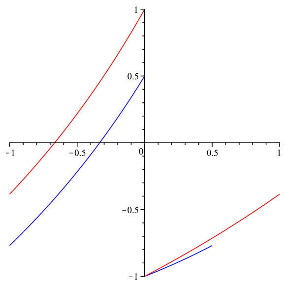
Figure 3. The graphs of $F_{a,v,c},G_{a,v,c}$ for $c=1.5$, $v=0.3$, and $a=1$ (above) and $a=0.5$ (below).

Proposition 3.4.

Suppose $c\in(0.5,1)$. For every pair $(a,v)\in\overset{\circ}{\Delta_{c}}$ set $\bar{v}=a\frac{\partial}{\partial a}+c\frac{\partial}{\partial v}$. Then

$$\inf_{z\in[-1,0]}\nabla_{\bar{v}}{F_{a,v,c}(z)}>0,\text{ and }\nabla_{\bar{v}}G_{a,v,c}(z)>0\text{ for all }z\in(0,a].$$

The similarly explicit computation is left to the reader. As a corollary of the Chain Rule, we have:

Proposition 3.5.

Suppose $(a,v)\in\overset{\circ}{\Delta}_{c}$ and $\bar{v}\in T_{a,v}\Delta_{c}$ with the properties

$$\inf_{z\in[-1,0]}\nabla_{\bar{v}}{F_{a,v,c}(z)}>0,\text{ and }\nabla_{\bar{v}}G_{a,v,c}(z)>0\text{ for all }z\in(0,a].$$

Then $\bar{v}\in{\cal C}_{a,v}$.

We remark:

Remark 3.1.

We do not know if the cone field ${\cal C}$ is non-empty when the restriction $c>0.5$ is removed. This is the only place in the proofs where this restriction is needed.

Moreover, it would be sufficient for our purposes to find tangent vectors which “lift” first return maps of renormalization intervals of a deeper level, instead of the first return map of $[-1,0]$. However, if $\tilde{F}$ and $\tilde{G}$ are replaced by a composition corresponding to such a return map, an explicit calculation of the directional derivative similar to the ones above becomes quite involved, and a brute force approach to finding a non-zero tangent vector with the desired property may become impractical.

The expansion properties of the cone field ${\cal C}$.

We begin by recalling how the composition operator acts on vector fields. For a pair of smooth functions $f$ and $g$, denote

$$\text{ Comp}(f,g)=f\circ g,$$

viewed as an operator $C^{\infty}\times C^{\infty}\to C^{\infty}$ and let $D\text{Comp}$ denote its differential. An elementary calculation shows that

(3.1) $$D\text{Comp}|_{(f,g)}:(\phi,\gamma)\to f^{\prime}\circ g\cdot\gamma+\phi\circ g.$$

The significance of the formula (3.1) for us lies in the following trivial observation: if $f$ and $g$ are both increasing functions, and the vector fields $\phi$ and $\gamma$ are non-negative, then

(3.2) $$\inf_{x}D\text{Comp}|_{(f,g)}(\phi,\gamma)\geq\inf_{x}\phi.$$

For a pair $\zeta_{a,v,c}$ with $(a,v)\in{\cal O}^{2}_{c}$ let us set

$$\lambda_{a,v,c}=F_{a,v,c}^{r_{0}}(-1)<0,$$

where, as before, $r_{i}$ denotes the height of ${\cal R}^{i}\zeta_{a,v,c}$. Note that

(3.3) $$\begin{split}{\cal T}\zeta_{a,v,c}=\Bigg{(}&-\frac{1}{\lambda_{a,v,c}}(F_{a,v,c}^{r_{0}}\circ G_{a,v,c})^{r_{1}}\circ F_{a,v,c}(-\lambda_{a,v,c}x),\\ &-\frac{1}{\lambda_{a,v,c}}F_{a,v,c}^{r_{0}}\circ G_{a,v,c}(-\lambda_{a,v,c}x)\Bigg{)}.\end{split}$$

We will require the following standard real a priori bound (see [KT1]):

Proposition 3.6.

There exists $\delta>0$ such that for every $(a,v)\in{\cal O}^{2}_{c}$,

$$\lambda_{a,v,c}>-\frac{1}{1+\delta}.$$

A key point for us is the following statement:

Proposition 3.7.

There exist $k\in{\mathbb{N}}$ and $\delta>0$ such that the following holds. Let $(a,v)\in{\cal O}_{c}^{2k}$ and let $\bar{v}\in{\cal C}_{a,v}$. Then

$$\nabla_{\bar{v}}A_{k,c}(a,v)>C(1+\delta)^{k},$$

where the constant $C>0$ depends only on $\bar{v}$.

Proof.

Let $\bar{v}=(\alpha,\nu)\in{\cal C}_{a,v}$. Consider a smooth deformation

(3.4) $$\zeta_{t}^{\bar{v}}=(F_{a+\alpha t,v+\nu t,c},G_{a+\alpha t,v+\nu t,c})\equiv(F_{t},G_{t}).$$

For $m\in{\mathbb{N}}$ let us denote

$${\cal T}^{m}\zeta_{t}^{\bar{v}}\equiv(F^{t}_{m},G^{t}_{m})\text{, and }p{\cal T}^{m}\zeta_{t}^{\bar{v}}\equiv(H^{t}_{m},K^{t}_{m}).$$

Let

$$\lambda_{m}^{t}\equiv|K^{t}_{m}(0)|.$$

An easy induction shows that

• $F^{t}_{k}(x)=\frac{1}{\lambda_{k}^{t}}H^{t}_{k}\circ(\lambda_{k}^{t}x);$

• $H_{k}^{t}(0)>0$.

A repeated application of (3.1) implies that

• $\frac{\partial}{\partial t}H^{t}_{k}(x)>\epsilon$ where $\epsilon=\inf_{x\in[0,a]}\nabla_{\bar{v}}F(x)$;

• $\frac{d}{dt}\lambda_{k}^{t}<0$.

We calculate:

$$\frac{\partial}{\partial t}\left(\frac{1}{\lambda_{k}^{t}}H_{k}^{t}(\lambda_{k}^{t}x)\right)=-\frac{\frac{d}{dt}\lambda_{k}^{t}}{(\lambda_{k}^{t})^{2}}H^{t}_{k}(\lambda_{k}^{t}x)+\frac{1}{\lambda_{k}^{t}}\left(\frac{\partial H_{k}^{t}(\lambda_{k}^{t}x)}{\partial t}+\frac{\partial H_{k}^{t}(x)}{\partial x}\frac{d\lambda_{k}^{t}}{dt}x\right).$$

Substituting $x=0$ and using $(a)-(d)$ we see that

$$\left.\frac{\partial}{\partial t}\right|_{t=0}\left.\left(\frac{1}{\lambda_{k}^{t}}H_{k}^{t}(\lambda_{k}^{t}x)\right)\right|_{x=0}=\nabla_{\bar{v}}A_{k,c}(a,v)\geq\frac{1}{\lambda_{k}^{0}}\epsilon.$$

Using the real a priori bound from Proposition 3.6 completes the proof. ∎

4. Constructing the renormalization horseshoe

Let us begin by making the following definition. For a finite sequence of natural numbers $r_{-2k},\ldots,r_{-1},r_{0},r_{1},\ldots,r_{2m}$ we set

$${\cal S}_{c,(r_{-2k},\ldots,r_{-1},r_{0},r_{1},\ldots,r_{2m})}\subset\Delta_{c}$$

to be the set of parameters $(a,v)\in{\cal O}^{2m}_{c}\cap{\cal T}^{2k}({\cal O}^{2k})$ where

$$(a,v)={\cal T}^{2k}(a_{-2k},v_{-2k})\text{ such that }\rho(\zeta_{a_{-2k},v_{-2k},c})=[r_{-2k},\ldots,r_{0},\ldots,r_{2m},\ldots].$$

For every inifnite sequence of natural numbers $(r_{0},r_{1},\ldots)$ let us denote

$$L_{c,(r_{0},r_{1},\ldots)}=\cap_{k\to\infty}{\cal S}_{c,(r_{0},r_{1},\ldots,r_{2k})}\subset\Delta_{c},\text{ so that }$$

$$L_{c,(r_{0},r_{1},\ldots)}=\{(a,v)\in\Delta_{c}\text{ such that }\rho(\zeta_{a,v,c})=[r_{0},r_{1},r_{2},\ldots]\in{\mathbb{R}}\setminus{\mathbb{Q}}\}.$$

We naturally identify the tangent space $T_{a,v}\Delta_{c}$ with ${\mathbb{R}}^{2}$ by

$$\iota:x\frac{\partial}{\partial a}+y\frac{\partial}{\partial v}\mapsto(x,y).$$

Proposition 4.1.

Let $c\in(0.5,2)\setminus\{1\}$. Then every set $L_{c,(r_{0},r_{1},\ldots)}$ is a continuous curve. Furthermore, for every point $(a,v)\in L_{c,(r_{0},r_{1},\ldots)}$ and every vector $\bar{v}\in{\cal C}_{a,v}$, the curve is locally disjoint from the line segment $\iota(\bar{v})\setminus\{(a,v)\}$.

Proof.

Let us start with the second assertion. Assume that for some $(a,v)\in L_{c,(r_{0},r_{1},\ldots)}$ there exists a point $(a^{\prime},v^{\prime})\in L_{c,(r_{0},r_{1},\ldots)}\cap\iota({\cal C}_{a,v})$. Denote $L$ the line segment connecting $(a,v)$ and $(a^{\prime},v^{\prime})$. Consider a linear map $\gamma:[0,1]\to L$ with $\gamma(0)=(a,v)$ and $\gamma(1)=(a^{\prime},v^{\prime})$. Assuming that $(a^{\prime},v^{\prime})$ is sufficiently close to $(a,v)$, we have

$$\frac{d}{dt}\bar{\gamma}(t)\in{\cal C}_{a(t),v(t)}\text{ for every }t\in[0,1]$$

by considerations of continuity. Hence, by Proposition 3.2 we have

$$\rho(\zeta_{a,v,c})<\rho(\zeta_{a^{\prime},v^{\prime},c}),$$

which contradicts our assumption.

Let us show that the set $L_{c,(r_{0},r_{1},\ldots)}$ is a continuous curve. We first present the argument for $c>1$. Note that for every $(a_{0},v_{0})\in\Delta_{c}$ the vertical line

$$\{v=v_{0}\}\subset\iota({\cal C}_{a_{0},v_{0}}).$$

Thus, the intersection

$$\alpha(v_{0})\equiv L_{c,(r_{0},r_{1},\ldots)}\cap\{v=v_{0}\}$$

contains at most one point.

Furthermore, consider the domain ${\cal D}_{c}\setminus{\cal O}^{1}_{c}$. On the upper boundary, $\{a=c\}$ we have $F_{a,v,c}(-1)=G_{a,v,c}(a)=0$. Hence, the rotation number $\rho(\zeta_{a,v,c})=[1,\infty]=1.$ On the other hand, on the lower boundary curve every $\zeta_{a,v,c}$ has a fixed point in $[-1,0]$, which is either the boundary point $-1$, or a point $w\in(-1,0)$ with $F_{a,v,c}^{\prime}(w)=1$. Thus the rotation number $\rho(\zeta_{a,v,c})=[\infty]=0$. Hence, by Intermediate Value Theorem, for $v>-1$ we have

$$\alpha(v)\neq\emptyset.$$

Finally, by continuity in the dependence of the rotation number on parameters, the parametrization

$$v\mapsto\alpha(v)\in L_{c,(r_{0},r_{1},\ldots)}$$

is continuous.

The proof for $c\in(0.5,1)$ is completely analogous , with the vertical lines $\{v=v_{0}\}$ replaced by $\{a=a_{0}\exp(v/c)\}$. We leave the details to the reader. ∎

We now use the Duality Theorem. For every backward-inifnite sequence of natural numbers $(\ldots,r_{-k},\ldots,r_{-2},r_{-1})$ let us denote

$$L_{c,(\ldots,r_{-2},r_{-1})}=\cap_{k\to\infty}{\cal S}_{c,(r_{-2k-1},\ldots,r_{-1})}\subset\Delta_{c}.$$

As a corollary of the Duality Theorem, we have:

Proposition 4.2.

Every

$$L_{1/c,(\ldots,r_{-2},r_{-1})}={\cal I}_{c}(L_{c,(r_{-1},r_{-2},\ldots)}).$$

In particular, every $L_{1/c,(\ldots,r_{-2},r_{-1})}$ is a continuous curve.

We are now ready to show:

Theorem 4.3.

Let $c\in(0.5,2)\setminus\{1\}$, and let $(r_{i})_{i\in{\mathbb{Z}}}$ be a periodic sequence of positive integers with period $2p,\;p\in{\mathbb{N}}$. Then there exists a unique $p$-periodic point $(a_{*},v_{*})$ of ${\cal T}_{c}$ with the property

$$\rho(\zeta_{a_{*},v_{*},c})=[r_{0},r_{1},\ldots,r_{2p-1},\ldots]\equiv\rho.$$

Furthermore, the orbit $(a_{*},v_{*})$ is hyperbolic with one stable and one unstable directions.

Finally, the curves

$$L_{c,(r_{0},r_{1},\ldots)}=W^{s}(a_{*},v_{*}),\text{ and }L_{c,(...,r_{-k},\ldots,r_{-1})}=W^{u}(a_{*},v_{*}).$$

Proof.

Elementary considerations of compactness and convergence imply that there exists a non-empty compact set

$$\Omega\subset L_{c,(r_{0},r_{1},\ldots)}$$

such that $({\cal T}_{c})^{p}(\Omega)=\Omega$, and moreover, for every $\zeta_{a,v,c}$ with $\rho(\zeta_{a,v,c})=\rho$ we have

$$({\cal T}^{c})^{pk}(\zeta_{a,v,c})\underset{k\to\infty}{\longrightarrow}\Omega.$$

Since a continuous mapping of a closed interval always has a fixed point, there exists at least one $p$-periodic point in $\Omega$, let us denote it $(a_{*},v_{*})$.

By Proposition 3.7, the matrix $D{\cal T}_{c}^{p}|_{(a_{*},v_{*})}$ has one expanding eigenvalue. By the Duality Theorem, it has a contracting eigenvalue. Hence, $(a_{*},v_{*})$ is a hyperbolic periodic orbit.

Let us prove that $L_{c,(r_{0},r_{1},\ldots)}=W^{s}(a_{*},v_{*})$ for $c\in(1,2)$. By continuity of the dependence of the rotation number on parameter,

$$W^{s}_{\text{loc}}(a_{*},v_{*})\subset L_{c,(r_{0},r_{1},\ldots)}.$$

Furthermore, both sets are continuous curves and hence locally coincide.

By construction of the renormalization operator, the global stable manifold $W^{s}(a_{*},v_{*})$ is a smooth sub-arc of $L_{c,(r_{0},r_{1},\ldots)}.$ Suppose that $W^{s}(a_{*},v_{*})$ is not the whole curve $L_{c,(r_{0},r_{1},\ldots)}$, and thus $W^{s}(a_{*},v_{*})$ has an endpoint $(x,y)\notin W^{s}(a_{*},v_{*})$. By invariance of $W^{s}(a_{*},v_{*})$ under ${\cal T}^{p}$, the point $(x,y)$ is also a $p$-periodic point of ${\cal T}$. The same argument as above implies that it is hyperbolic and that $W^{s}_{\text{loc}}(x,y)$ is a smooth sub-arc in $L_{c,(r_{0},r_{1},\ldots)}$. Hence

$$W^{s}_{\text{loc}}(x,y)\cap W^{s}(a_{*},v_{*})\neq\emptyset,$$

and we have arrived at a contradiction.

The argument for $c\in(0.5,1)$ is again completely analogous, with the lines $\{v=v_{0}\}$ replaced by curves $\{a=a_{0}\exp(v/c)\}$.

As a consequence,

$$\Omega=\{(a_{*},v_{*})\}.$$

Finally, the statement $L_{c,(...,r_{-k},\ldots,r_{-1})}=W^{u}(a_{*},v_{*})$ follows by the Duality Theorem.

∎

Let us formulate a few corollaries:

Proposition 4.4.

For every periodic sequence $(r_{i})_{i\in{\mathbb{Z}}}$, the curves $L_{c,(r_{0},r_{1},\ldots)}$ and $L_{c,(...,r_{-k},\ldots,r_{-1})}$ are $C^{\omega}$-smooth.

The following statement follows from the results of [KT2]:

Proposition 4.5.

For every periodic sequence $(r_{i})_{i\in{\mathbb{Z}}}$, the curves $L_{c,(r_{0},r_{1},\ldots)}$ and $L_{c,(...,r_{-k},\ldots,r_{-1})}$ intersect uniformly transversely.

Note (see Remark 2.1) that for orbits of bounded type the uniformity of transversality of intersection follows by considerations of compactness, without appealing to [KT2].

Proposition 4.6.

For every $c\in(0.5,2)\setminus\{1\}$ and every bi-infinite sequence of natural numbers $(r_{i})_{i\in{\mathbb{Z}}}$ there exists a unique point $(a,v)=(a,v)_{(r_{i})_{i\in{\mathbb{Z}}}}\in\Delta_{c}$ such that:

• $\rho(\zeta_{a,v,c})=[r_{0},r_{1},\ldots]$;

• for every $m\in{\mathbb{N}}$ the rotation number

  $$\rho({\cal T}_{c}^{-m}(\zeta_{a,v,c}))=[r_{-2m},\ldots,r_{0},r_{1},\ldots].$$

Proof.

Let us show that the intersection of the curves

$$\Omega\equiv L_{c,(\ldots,r_{-2},r_{-1})}\cap L_{c,(r_{0},r_{-1},\ldots})$$

is non-empty. For every even $n\in{\mathbb{N}}$ let

$$\rho_{n}\equiv[r_{-n},\ldots,r_{n-1},r_{-n},\ldots,r_{n-1},\ldots],$$

and let $(a_{n},v_{n})$ be the unique ${\cal T}_{c}$-periodic point with period $n$ and

$$\rho(\zeta_{a_{n},v_{n},c})=\rho_{n}.$$

Then, by continuity of the rotation number, every limit point of the sequence $\{({\cal T}_{c})^{n/2}(a_{n},v_{n})\}$ lies in $\Omega$. Thus, $\Omega\neq\emptyset.$

Furthermore, let us show that for each bi-infinite sequence $(r_{i})_{i\in{\mathbb{Z}}}$ the intersection $L_{c,(\ldots,r_{-2},r_{-1})}\cap L_{c,(r_{0},r_{-1},\ldots})$ consists of a single point. We first note that in the case when $(r_{i})_{i\in{\mathbb{Z}}}$ is a periodic sequence, the curves $L_{c,(\ldots,r_{-2},r_{-1})}$ and $L_{c,(r_{0},r_{-1},\ldots})$ are the unstable and stable manifolds of the unique periodic orbit with rotation number $[r_{0},r_{1},\ldots]$. If these manifolds have a homoclinic intersection point, then neither one of them could be a smooth curve, which would contradict Theorem 4.3.

The general case now follows by Proposition 4.5 and considerations of continuity.

∎

Let us denote ${\cal A}_{c}$ the collection of all pairs $(a,v)_{(r_{i})_{i\in{\mathbb{Z}}}}\in\Delta_{c}$. By construction, we have:

Proposition 4.7.

The map $\iota:\Sigma_{\mathbb{N}}\to{\cal A}_{c}$ given by $\iota:(r_{i})_{i\in{\mathbb{Z}}}\mapsto(a,v)_{(r_{i})_{i\in{\mathbb{Z}}}}\in\Delta_{c}$ is a homeomorphism.

By Proposition 4.6,

(4.1) $$\rho(\zeta_{\iota(r_{i}),c})=[r_{0},r_{1},\ldots]\text{ and }\iota^{-1}\circ{\cal T}_{c}\circ\iota=\sigma^{2}.$$

Denote ${\cal P}_{c}$ the dense subset of ${\cal A}_{c}$ consisting of periodic orbits. For every periodic sequence $(r_{i})_{i\in{\mathbb{Z}}}$, consider the tangent vector field $T^{s}$ of the curves $L_{c,(r_{0},r_{1},\ldots)}$, and the tangent vector field $T^{u}$ of $L_{c,(...,r_{-k},\ldots,r_{0})}$. By a simple diagonal convergence process, $T^{s}$ and $T^{u}$ can be extended to all of ${\cal A}_{c}$ as a $D{\cal T}_{c}$-invariant splitting of the tangent bundle. Furthermore, Proposition 3.7 implies that $D{\cal T}$ uniformly expands $T^{u}$, and by Duality Theorem, $D{\cal T}$ uniformly contracts $T^{s}$. Hence:

Proposition 4.8.

For $c\in(0.5,2)\setminus\{1\}$ the set ${\cal A}_{c}$ is uniformly hyperbolic, with one stable and one unstable direction. The curves $L_{c,(r_{0},r_{1},\ldots)}$ and $L_{c,(...,r_{-k},\ldots,r_{0})}$ are the stable and the unstable foliation of ${\cal A}_{c}$ respectively.

Thus,

Proposition 4.9.

The curves $L_{c,(r_{0},r_{1},\ldots)}$ and $L_{c,(...,r_{-k},\ldots,r_{0})}$ are $C^{\omega}$-smooth.

References

- [KK] K. Khanin and D. Khmelev, ”Renormalizations and rigidity theory for circle homeomorphisms with singularities of the break type”, Comm. Math. Phys., 235 (2003), 69-124.
- [KT1] K. Khanin, A. Teplinsky, “Robust rigidity for circle diffeomorphisms with singularities”, Invent. Math., 169(2007), 193-218
- [KT2] K. Khanin, A. Teplinsky, “Renormalization horseshoe and rigidity theory for circle diffeomorphisms with breaks”, Commun. Math. Phys. 320(2013), 347-377
- [KV] K. M. Khanin, E. B. Vul, “Circle homeomorphisms with weak discontinuities”. In proc. of Dynamical systems and statistical mechanics (Moscow, 1991), 57-98. Amer. Math. Soc, Providence, RI, 1991.
- [VK] E. B. Vul and K. M. Khanin, ”Homeomorphisms of the circle with singularities of break type”, Uspekhi Mat. Nauk, 45:3 (1990), 189 190; English transl. Russian Math. Surveys, 45:3 (1990), 229-230
- [Ya1] M. Yampolsky, “The attractor of renormalization and rigidity of towers of critical circle maps”, Commun. Math. Physics, 218(2001), 537-568.
- [Ya2] M. Yampolsky, “Hyperbolicity of renormalization of critical circle maps”, Publ. Math. Inst. Hautes Etudes Sci. No. 96 (2002), 1-41
- [Ya3] M. Yampolsky, “Global renormalization horseshoe for critical circle maps”, Commun. Math. Physics, 240(2003), 75–96.