Bayesian naturalness of the CMSSM and CNMSSM

Abstract

The recent discovery of the $125.5$ GeV Higgs boson at the LHC has fuelled interest in the Next-to-Minimal Supersymmetric Standard Model (NMSSM) as it may require less fine-tuning than the minimal model to accommodate such a heavy Higgs. To this end we present Bayesian naturalness priors to quantify fine-tuning in the (N)MSSM. These priors arise automatically as Occam razors in Bayesian model comparison and generalize the conventional Barbieri-Giudice measure. In this paper we show that the naturalness priors capture features of both the Barbieri-Giudice fine-tuning measure and a simple ratio measure that has been used in the literature. We also show that according to the naturalness prior the constrained version of the NMSSM is less tuned than the CMSSM.

I Introduction

Naturalness is a guiding principle in search of new physics beyond the Standard Model (SM) Giudice:2013yca . A naturalness problem arises in the SM since the Higgs mass is sensitive to new physics above the electroweak scale and only delicate fine-tuning amongst the fundamental parameters can stabilize it. Supersymmetry cancels the quadratic divergence in the Higgs mass improving naturalness. In the Minimal Supersymmetric Standard Model (MSSM), however, the large radiative corrections that lift the Higgs mass reintroduce some fine-tuning Giudice:2013yca .

The recent Higgs discovery makes the little hierarchy problem more acute Aad:2012tfa ; Chatrchyan:2012ufa . This triggered interest in supersymmetric models that can naturally accommodate a 125.5 GeV Higgs, such as the Next-to-Minimal Supersymmetric Standard Model (NMSSM). A new $F$-term in the NMSSM, proportional to the Higgs-singlet coupling $\lambda$, boosts the tree level Higgs mass. Natural NMSSM scenarios have been presented where $\lambda$ remains perturbative up to the GUT scale King:2012tr , and in $\lambda$-SUSY scenarios where $\lambda$ is only required to remain perturbative up to a scale just above TeV Gherghetta:2012gb .

To show that the NMSSM is less fine-tuned than the MSSM one has to quantify naturalness. Conventional fine-tuning measures rely on the sensitivity of the weak scale to changes in the fundamental parameters of the model. In Bayesian model comparison such measure arises automatically as a Jacobian of the variable transformation from the Higgs vacuum expectation values (VEVs) to the fundamental parameters Allanach:2007qk ; Cabrera:2008tj ; Cabrera:2009dm ; Ghilencea:2012gz ; Ghilencea:2012qk ; Fichet:2012sn .

In this paper we present the NMSSM fine-tuning prior. We examine how the prior varies with the parameter of the constrained NMSSM and compare it to the Barbieri-Giudice measure Ellis:1986yg ; Barbieri:1987fn and the simple ratio measure Baer:2012up ; Baer:2012cf ; Baer:2013bba ; Baer:2013gva . In a longer companion paper we will provide the full details of the derivation of the presented Jacobian and carry out a detailed numerical analysis for the unconstrained NMSSM.

II Measuring fine-tuning

Naturalness of supersymmetric models is quantified in various different ways in the literature today. One of the simplest fine-tuning measures is Baer:2012up ; Baer:2012cf ; Baer:2013bba ; Baer:2013gva

$$\Delta_{EW}=\max\{|C_{i}|/(m_{Z}^{2}/2)\},$$ (1)

which is based on the electroweak symmetry breaking (EWSB) condition of the MSSM

$$\frac{m_{Z}^{2}}{2}=\frac{(m_{H_{d}}^{2}+\delta m_{H_{d}}^{2})-(m_{H_{u}}^{2}+\delta m_{H_{u}}^{2})\tan^{2}\beta}{\tan^{2}\beta-1}-\mu^{2},$$ (2)

where $\delta m_{H_{u}}^{2}$ and $\delta m_{H_{d}}^{2}$ are the one loop tadpole corrections to the tree level minimisation conditions. The $C_{i}$ ($i$ = $m_{H_{u}}^{2}$, $m_{H_{d}}^{2}$, $\delta m_{H_{u}}^{2}$, $\delta m_{H_{d}}^{2}$, $\mu^{2}$) in Eq. (1) are the additive terms appearing in Eq. (2), specified by the index.

An alternative and widely used measure of naturalness, the Barbieri-Giudice measure Ellis:1986yg ; Barbieri:1987fn , accounts for correlations between the terms in Eq. (2),

$$\Delta_{BG}(p_{i})=\left|\frac{\partial\ln m_{Z}^{2}}{\partial\ln p_{i}^{2}}\right|,\;\;\;\Delta_{BG}=\max\{\Delta_{BG}(p_{i})\}.$$ (3)

where $p_{i}$ are the input parameters of the model, for some chosen parametrisation. Alternatively some authors combine the $\Delta_{BG}(p_{i})$ by summation in quadrature: $\tilde{\Delta}_{BG}^{2}=\sum_{i}{\Delta^{2}_{BG}(p_{i})}$. The Barbieri-Giudice measure quantifies the sensitivity of the observable $m_{Z}^{2}$ to the parameters $\{p_{i}\}$, e.g. $\Delta_{BG}(p_{i})=10$, means a 1 percent change in $p_{i}$ leads to 10 percent change in $m_{Z}^{2}$.

Alternative measures have also been proposed Anderson:1994tr ; Anderson:1994dz ; Athron:2007ry but these are not considered here.

In Bayesian model comparison the Barbieri-Giudice measure arises automatically as the special case of a more general fine-tuning measure Allanach:2007qk ; Cabrera:2008tj ; Cabrera:2009dm ; Ghilencea:2012gz ; Ghilencea:2012qk ; Fichet:2012sn . In this framework the odds ratio between competing models is defined in terms of the ratio of marginal likelihoods, or evidences

$$\mathcal{E}(\mathcal{D},\mathcal{M})=\int_{\Omega}\mathcal{L}_{\mathcal{D}}(p_{i};\mathcal{M})\pi(p_{i}|\mathcal{M})\,d^{N}\!p_{i}.$$ (4)

Here $\mathcal{L}_{\mathcal{D}}$ is the likelihood function for the data $\mathcal{D}$, quantifying the goodness of fit of the model $\mathcal{M}$ to the data at each point in the model’s $N$ dimensional parameter space $\{p_{i}\}$. The distribution $\pi$ assigns a probability density to each parameter space point as assessed prior to the data $\mathcal{D}$ being learned, and $\Omega$ is the domain over which this pdf is non-zero.

However, for computing likelihoods, and for scanning, the parameter set $\{p_{i}\}$ on which $\pi$ is most sensibly defined is often less convenient to work with than a set of derived parameters or “observables” $\mathcal{O}_{i}$, some of which, such as $m_{Z}$, may be precisely measured. Switching to these new variables distorts the prior density, as quantified by the Jacobian of the transformation,

$$d^{N}\!p_{i}=\left|\frac{\partial p_{i}}{\partial\mathcal{O}_{j}}\right|d^{N}\mathcal{O}_{j}.$$ (5)

In the new coordinates the sharply known observables can be easily marginalised out, reducing the dimension of the parameter space. Choosing logarithmic priors on $\{p_{i}\}$ and neglecting constants which divide out of evidence ratios gives

$$\mathcal{E}(\mathcal{D},\mathcal{M})=\frac{1}{V_{\log}}\int_{\Omega^{\prime}}\mathcal{L}_{\mathcal{D}^{\prime}}\left.\frac{1}{\Delta_{J}}\right|_{\hat{\mathcal{O}}=\hat{\mathcal{D}}}\frac{d^{N-r}\mathcal{O}^{\prime}_{j}}{\mathcal{O}^{\prime}_{j}}$$ (6)

where $\hat{\mathcal{O}}$ and $\hat{\mathcal{D}}$ are the $r$ observables and data used in the dimensional reduction, $\mathcal{D^{\prime}}$ and $\mathcal{O^{\prime}}$ are the data and observables remaining, $V_{\log}=\int_{\Omega}d^{N}\!p_{i}/p_{i}$ is the “logarithmic” volume of the parameter space in the original coordinates, $\Omega^{\prime}$ is the part of $\Omega$ orthogonal to the removed dimensions and

$$\Delta_{J}=\left|\frac{\partial\ln\mathcal{O}_{j}}{\partial\ln p_{i}}\right|.$$ (7)

If log priors are not used extra terms will also appear. $\Delta_{J}^{-1}$ appears in the evidence through the transformation of the prior density to new coordinates, $\pi(\mathcal{O}_{j})=\Delta_{J}^{-1}(p_{i}/\mathcal{O}_{j})\pi(p_{i})=\Delta_{J}^{-1}(1/\mathcal{O}_{j})$. The last equality follows from initially choosing log priors (neglecting normalisation constants). One can then scan the derived parameters using log priors with $\Delta_{J}^{-1}$ as an “effective” prior weighting of the likelihood, and obtain a posterior weighting of points compatible with the original prior.

Clearly all parameters do not have to be exchanged for observables. When a single parameter $p^{2}$ is exchanged for $\mathcal{O}_{i}=m_{Z}^{2}$, $\Delta_{J}$ is the Barbieri-Giudice sensitivity, $\Delta_{BG}(p_{i})$, in Eq. (3). In general more than one low energy observable is involved in the transformation, so the relevant Jacobian contains more structure than the Barbieri-Giudice measure.

For example most MSSM spectrum generators take $(m_{Z},\tan\beta,m_{t})$ as input instead of $(\mu,B,y_{t})$; the transformation $(\mu,B,y_{t})\to(m_{Z},\tan\beta,m_{t})$ thus emerges as sensible choice which can quantify unnatural cancellations required to keep $m_{Z}\ll M_{SUSY}$. The resulting Jacobian

$$\Delta_{J}^{\textrm{CMSSM}}= \left|\frac{\partial\ln(m_{Z}^{2},\tan\beta,m_{t}^{2})}{\partial\ln(\mu_{0}^{2},B_{0},y_{0}^{2})}\right|$$ (8)

$$= \left(\frac{M_{Z}^{2}}{2\mu^{2}}\frac{B}{B_{0}}\frac{\tan^{2}\beta-1}{\tan^{2}\beta+1}\frac{\partial\ln y_{t}^{2}}{\partial\ln y_{0}^{2}}\right)^{-1},$$

automatically includes $\Delta_{BG}(\mu_{0},B_{0},y_{0})$ as a single column (where the subscript $0$ denotes the GUT scale parameter value). The extra columns of $\Delta_{J}$ account correctly for correlations between the $m_{Z}$ related tunings and those coming from the Higgs VEVs and top mass. The Yukawa RGE factor $\frac{\partial\ln y_{t}^{2}}{\partial\ln y_{0}^{2}}$ is constant over the CMSSM parameter space at the 1-loop level and so we neglect it. It is close to one anyway so the constant shift this induces in the logarithms of tunings reported in our numerical analysis is very small.

Importantly, we see that Eq. (6) captures much of the intuition behind the fine-tuning problem. We see that to be preferred in a Bayesian test, a model needs to have overlapping regions of both high likelihood and low fine-tuning (and that this region should not be too small relative to the prior volume $V_{\log}$, which is itself a naturalness-style requirement).

The extension of $\Delta_{J}$ to the NMSSM goes as follows. As indicated above, $\Delta_{J}$ in practice depends on the particular spectrum generator of choice as well as the definition of the model. For concreteness we consider a constrained version of the NMSSM (CNMSSM), defined at the GUT scale to have a universal gaugino mass, $M_{1/2}$; a universal soft trilinear mass, $A_{0}$ and all MSSM-like soft scalar masses equal to $m_{0}$, but the new soft singlet mass, $m_{S}$ is left unconstrained at the GUT scale. Thus the model has the parameter set $(M_{0},M_{1/2},A_{0},\lambda_{0},\kappa_{0},m_{S})$ which can be compared to the CMSSM set of $(M_{0},M_{1/2},A_{0},\mu_{0},B_{0})$.

The effective prior weighting we present is chosen to be suitable for Bayesian studies with numerical implementation in both the spectrum generator NMSPEC in the NMSSMTools 4.1.2 package and the newly developed spectrum generator Next-to-Minimal SOFTSUSY Allanach:NMSOFTSUSY distributed with SOFTSUSY 3.4.0. For a constrained model as defined above the spectrum generators trade $(\lambda_{0},\kappa_{0},m_{S}^{2})$ for $(\lambda,m_{Z},\tan\beta)$ giving the user the input parameters of $(M_{0},M_{1/2},m_{Z},\tan\beta,A_{0},\lambda)$, i.e. just $\lambda$ in addition to the usual CMSSM inputs used in spectrum generators.

This transformation gives rise to a Jacobian,

$$d\lambda_{0}d\kappa_{0}dm_{S_{0}}^{2}=J_{\mathcal{T}_{0}}d\lambda dM_{z}^{2}d\tan\beta$$ (9)

which may be written as,

$$J_{\mathcal{T}_{0}} =J_{\mathcal{T}_{\kappa m_{S}}^{\lambda}}J_{RG}$$ (10)

$$=\begin{vmatrix}&\frac{\partial\kappa}{\partial m_{Z}^{2}}&\frac{\partial m_{S}^{2}}{\partial m_{Z}^{2}}&\\ &\frac{\partial\kappa}{\partial\tan\beta}&\frac{\partial m_{S}^{2}}{\partial\tan\beta}&\end{vmatrix}_{\lambda}\begin{vmatrix}&\frac{\partial\lambda_{0}}{\partial\lambda}&\frac{\partial\kappa_{0}}{\partial\lambda}&\\ &\frac{\partial\lambda_{0}}{\partial\kappa}&\frac{\partial\kappa_{0}}{\partial\kappa}&\end{vmatrix}\left|\frac{\partial m_{S_{0}}^{2}}{\partial m_{S}^{2}}\right|$$

The Jacobian $J_{\mathcal{T}_{\kappa m_{S}}^{\lambda}}$ can be rewritten in terms of simpler coefficients embedded in the determinant of a three by three matrix,

$$J_{\mathcal{T}_{\kappa m_{S}}^{\lambda}} =\frac{1}{b_{1}}\begin{vmatrix}&b_{1}&e_{1}&a_{1}&\\ &b_{2}&e_{2}&a_{2}&\\ &b_{3}&e_{3}&a_{3}&\end{vmatrix}.$$ (11)

The coefficients appearing in this expression are given in the appendix. $J_{RG}$ transforms the input parameters from the GUT scale to the electroweak scale, and factorises as shown due to the supersymmetric non-renormalization theorem. The subscript $\lambda$ indicates that this parameter is kept constant in the derivatives.

As happens in going from Eq. 5 to Eq. 6 we can choose to work with the logarithms of parameters (as is natural if we choose logarithmic priors) so that we obtain a new factor in the denominator, which is the inverse of the Jacobian with logarithms inserted inside the derivatives. This gives us

$$\Delta_{J}^{\textrm{CNMSSM}} =\left|\frac{\partial\ln(m_{Z}^{2},\tan\beta,\lambda)}{\partial\ln(\kappa_{0},m_{S_{0}}^{2},\lambda_{0})}\right|$$ (12)

$$=\frac{\kappa_{0}m_{S_{0}}^{2}\lambda_{0}}{m_{Z}^{2}\tan\beta\lambda}J_{\mathcal{T}_{0}}^{-1}$$

It is well known that the top quark Yukawa coupling can play a significant role in fine-tuning so we also considered this by extending the transformation to include the top quark mass and (unified) Yukawa coupling, $(\kappa_{0},m_{S_{0}}^{2},\lambda_{0},y_{0})\rightarrow(m_{Z}^{2},\tan\beta,\lambda,m_{t})$. Nonetheless as was already observed in the MSSM case Cabrera:2008tj ; Cabrera:2009dm , we found that all the derivatives, other than $\frac{\partial m_{t}}{\partial y_{t}}$, that involve $m_{t}$ and $y_{t}$ cancel, so this only changes the Jacobian by a single multiplicative factor of $\frac{\partial m_{t}}{\partial y_{t}}$. Finally when logarithmic priors are chosen this factor will disappear entirely because $\frac{\partial\ln m_{t}}{\partial\ln y_{t}}=1$, and the Yukawa RGE factor $\frac{\partial\ln y_{t}}{\partial\ln y_{0}}$ is the same order one constant (at 1-loop) as in the CMSSM case so we neglect it.

Therefore we write our NMSSM Jacobian based tuning measure as,

$$\Delta_{J}^{\textrm{CNMSSM}}=\left|\frac{\partial\ln(m_{Z}^{2},\tan\beta,\lambda,m_{t}^{2})}{\partial\ln(\kappa_{0},m_{S_{0}}^{2},\lambda_{0},y_{0}^{2})}\right|,$$ (13)

with the additional transformation between $m_{t}$ and $y_{0}$ included to emphasise that we have also considered these, since the cancellation will prove to be rather important (in both the MSSM and NMSSM) when we compare against the Barbieri-Giudice tuning measure in the focus point (FP) region. There we will show that due to this cancellation we do not see a large tuning penalty in the much discussed FP regionFeng:2011aa ; Feng:2012jfa ; Feng:1999zg ; Feng:1999mn , which appears in the Barbieri-Giudice measure when one includes $y_{t}$ as a parameter.

The expression given here is formally the Jacobian which should be used in the Bayesian analysis of any NMSSM model when $(\lambda_{0},\kappa_{0},m_{S_{0}}^{2},y_{0}^{2})$ are traded for $(m_{Z}^{2},\tan\beta,\lambda,m_{t}^{2})$. At the same time $\Delta_{J}^{\textrm{CNMSSM}}$ can be interpreted as a measure of the naturalness of the NMSSM, which may be applied to the CNMSSM, the general NMSSM and $\lambda$-SUSY scenarios.

Interestingly, as it was argued in the recent literature Ghilencea1311.6144 , the above Jacobians can also be considered to measure fine-tuning from a purely frequentist perspective. In this context the same Jacobians appear as part of the likelihood function after one includes observables in $\chi^{2}$ which are related to the scale of electroweak symmetry breaking, such as the mass of the $Z$ boson. Just as above, the variable transformation from these observables to fundamental parameters induces the Jacobian, which can be interpreted as a part of the likelihood that measures the sensitivity of the predicted electroweak scale to the fundamental parameters of the model. Steep derivatives of the relevant observables with respect to the chosen fundamental parameters signal a strongly peaked likelihood function, indicating that $\chi^{2}$ drops off rapidly from the best fit value as those parameters are changed, which is of course indicative of high fine-tuning. The Bayesian perspective offers additional insight into the reasons we might dislike such behaviour in our likelihood functions, since in the frequentist case the actual best-fit $\chi^{2}$ does not suffer a penalty for any tuning observed in its vicinity, while in the Bayesian case there is a clear and direct penalty originating from the small prior–likelihood overlap that such behaviour implies.

III Numerical analysis

For our numerical analysis we use SOFTSUSY 3.3.5 for the MSSM Allanach:2001kg , and NMSPEC Ellwanger:2006rn in NMSSMTools 4.1.2 for the NMSSM. Next-to-Minimal SOFTSUSY Allanach:NMSOFTSUSY was still in development during this analysis but was used to cross check the spectrum for certain points. MultiNest 3.3 was used for scanning Feroz:2008xx ; Feroz:2007kg . Both spectrum generators used here provide $\Delta_{BG}$ with renormalization group flow improvement. For $\Delta_{BG}$ in the CMSSM we include individual sensitivities, $\Delta_{BG}(p_{i})$, for the set of parameters $M_{0},M_{1/2},A_{0},\mu,B,y_{t}$. For the CNMSSM we use the set $M_{0},M_{1/2},A_{0},\lambda,\kappa,y_{t}$.

First we examine how the tuning measures vary with $M_{0}$ and $M_{1/2}$, without requiring a $125$ GeV Higgs. We fix $\tan\beta=10$, where the extra NMSSM F-term contribution is small, but there is interesting focus point (FP) behavior Feng:2011aa ; Feng:2012jfa ; Feng:1999zg ; Feng:1999mn . Previous studies Kowalska:2012gs show that large and negative $A_{0}$ is favoured, so to simplify the analysis here and throughout we choose $A_{0}=-2.5$ TeV.

The results for the CMSSM are shown in FIG. 1. The value of $\Delta_{EW}$ is governed by the $m_{H_{u}}^{2}$ and $\mu^{2}$ contributions since $m_{Z}^{2}/2\approx-\overline{m}_{H_{u}}^{2}-\mu^{2}$, where $\overline{m}_{H_{u}}^{2}$ includes the radiative corrections. In general $\Delta_{EW}$ is dominated by $\mu^{2}$, while the crossover to the $m_{H_{u}}^{2}$ dominance occurs in the vicinity of the EWSB boundary.

For this measure there is low fine-tuning even at large $M_{0}$. This may seem counterintuitive, but for $\tan\beta=10$ at large $M_{0}$ we are close to a FP region. In this region the dependence on $M_{0}$ which appears from RG evolution of $m_{H_{u}}$ vanishes. For example in the CMSSM semi-analytical solution to the renormalisation group equations (RGEs),

$$m_{H_{u}}^{2} = c_{1}M_{0}^{2}+c_{2}M_{1/2}^{2}+c_{3}A_{0}^{2}+c_{4}M_{1/2}A_{0},$$ (14)

the coefficients $c_{i}$ are functions of Yukawa and gauge couplings, and $\tan\beta$ and $c_{1}$ can be close to zero. Such regions then appear to have low fine-tuning even with large $M_{0}$ since the small size of $c_{1}$ means there is no need to cancel the large $M_{0}$ in Eq. (2) to obtain the correct $m_{Z}^{2}$.

In $\Delta_{BG}$, however, the sensitivity to the top quark Yukawa coupling is included. Since the RG coefficients depend on this Yukawa coupling, the large stop corrections from the RGEs that feed into $m_{H_{u}}^{2}$ lead to a large $\Delta_{BG}(y_{t})$ even in the focus point region. $\Delta_{EW}$ is not sensitive to this effect since it does not take into account such RG effects.

Figure 1: Fine tuning measures $\Delta_{BG}$ (top), $\Delta_{J}$ (middle), $\Delta_{EW}$ (bottom) in the $M_{0}$ vs. $M_{1/2}$ plane for $A_{0}=-2.5$ TeV, $\tan\beta=10$ and sgn($\mu$)=1 in the CMSSM. The color code quantifies the value of $\Delta_{EW}$ and $\Delta_{J}$. Since $\Delta_{BG}$ is dominated by the $\mu$ derivative it is low in the small $M_{0}$ and $M_{1/2}$ region. Although $\Delta_{BG}$, by definition, is formally part of $\Delta_{J}$ the numerical behaviour of the latter is similar to that of $\Delta_{EW}$. All massive parameters are in GeV unit. No experimental constraints applied except that the lightest supersymmetric particle is electrically neutral and the EWSB condition is satisfied.

Figure 2: Same as FIG. 1 except for the constrained NMSSM. $A_{0,\kappa,\lambda}=-2.5$ TeV and $\tan\beta=10$ are assumed. $\lambda$ is sampled from the range [0,0.8].

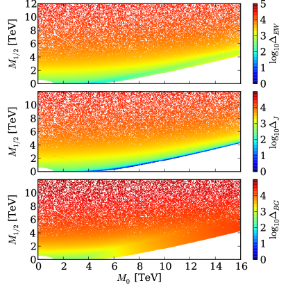
Interestingly $\Delta_{J}^{\textrm{CMSSM}}$ exhibits similar behavior to $\Delta_{EW}$ despite containing derivatives from $\Delta_{BG}$. This is because $\Delta_{J}^{\textrm{CMSSM}}$ does not contain the derivative of $m_{Z}$ with respect $y_{t}$. When one computes the Jacobian for Eq. (8) the derivative of $y_{t}$ with respect to $m_{Z}$ cancels out, leaving only the derivatives $\frac{\partial\mu}{\partial M_{z}}\frac{\partial B\mu}{\partial t}\frac{\partial y_{t}}{\partial m_{t}}$ in the Jacobian. As a result $\Delta_{J}$ in the MSSM can remain small in the focus point region.

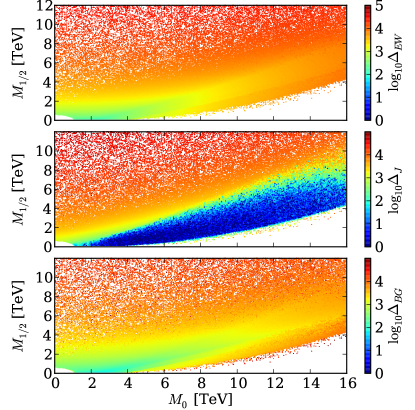
Fine tuning measures for the CNMSSM are shown in FIG. 2. Here $\Delta_{J}^{\textrm{CNMSSM}}$ is defined by Eq. (13) and $\Delta_{BG}$ is defined by Eq. (3), while $\Delta_{EW}$ is defined the same as for the MSSM. The parameter $\mu$ dominates electroweak tuning, $\Delta_{EW}$, throughout the $M_{0}$ vs. $M_{1/2}$ plane. Since $\mu$ values and related derivatives are similar in the CMSSM and CNMSSM the fine-tuning measures are qualitatively similar for the two models.

As in the CMSSM the Jacobian derived tuning $\Delta_{J}$ increases with $M_{1/2}$, as anticipated since for large $M_{1/2}$ large cancellation is required to keep $m_{Z}$ light. Again though at large $M_{0}$ $\Delta_{J}$ can still be low seeming to favour this FP region, which is a result of the same cancellation as happened in the MSSM case occurring in our new NMSSM Jacobian.

Interestingly the region where the tuning can be very low extends further in the NMSSM. Note this is not a result of raising the Higgs mass with $\lambda$ since we impose no Higgs constraint yet and have large $\tan\beta$. However $\lambda$ is varied across the plane and affects the EWSB condition and the renormalization group evolution. However since the number of parameters are different in the CNMSSM and CMSSM, to determine whether the CNMSSM is preferred over the CMSSM, we have to compare Bayesian evidences.

Figure 3: Fine tuning with respect to $m_{h^{0}}$ for the CMSSM (upper) and CNMSSM (lower). $A_{0}=-2.5$ TeV and $\tan\beta=10$ for both models.

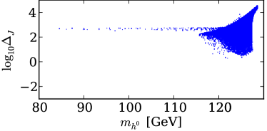
Since the focus point region allows small $\Delta_{EW}$ and $\Delta_{J}$ in the large $M_{0}$ region it is possible to have a relatively heavy lightest Higgs and small $\Delta_{J}$. This is illustrated in FIG. 3. Note also that in the NMSSM case there is no tuning preference for large $\lambda$ since the new F-term contribution goes like $\lambda^{2}v^{2}\sin^{2}2\beta$ and is therefore suppressed at large $\tan\beta$. Nonetheless in the focus region in both the CMSSM and CNMSSM one can have a $125$ GeV without an enormous penalty from effective prior weighting $\Delta_{J}$.

However the lowest tuning is when $M_{1/2}$ is smallest and this region is strongly constrained by squark and gluino searches. The important message, nonetheless, is that the Higgs mass measurement has a low impact on naturalness in the focus point region. Therefore the effect of the Higgs mass measurement may not be as severe on our degree of belief as we would expect from $\Delta_{BG}$, even in the MSSM. A caveat to this optimistic statement is that from looking at $\Delta_{J}$ alone one cannot know if the focus point scenarios will be suppressed by other factors in the full Bayesian analysis. This can only be determined by carrying out that analysis.

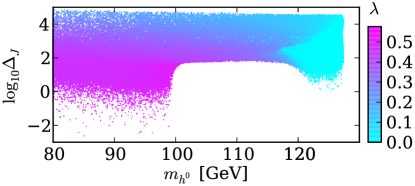
Away from this special FP region the Higgs mass measurement has a large impact and the extra $F$-term of the NMSSM can play a vital role. In Fig. 4 we compare the Higgs mass against fine-tuning for $\tan\beta=3$ in both the CMSSM and the CNMSSM. Here the extra NMSSM F-term can give a larger contribution to the SM-like Higgs mass and it is precisely this effect which leads to expectations of increased naturalness in the NMSSM.

In the MSSM the tree level upper bound reduces rapidly at small $\tan\beta$. Therefore we do not find any CMSSM solutions with a lightest Higgs mass above $120$ GeV in FIG. 4. The maximum achievable mass of the lightest Higgs has $\Delta_{J}\approx 10^{5}$. By comparison the same mass for the lightest Higgs in the CNMSSM can be achieved with $\Delta_{J}$ between $10^{2}-10^{3}$. So according to the naturalness prior measure $\Delta_{J}$ the tuning is reduced compared to the CMSSM for heavier Higgs masses.

Nonetheless for $m_{h^{0}}>m_{Z}$ on contours of fixed $\lambda$, $\Delta_{J}$ increases with the lightest Higgs mass and the minimum $\Delta_{J}$ starts increasing significantly when the lightest Higgs mass is pushed above $115$ GeV. As expected the largest Higgs masses are found for sizable $\lambda$. This demonstrates that for the new Jacobian naturalness measure for the NMSSM the additional F-term contribution in the NMSSM really does decreasing fine-tuning of the model as one increases $\lambda$, strongly supporting previous that this mechanism can reduce fine-tuning in the low $\tan\beta$ region of the NMSSM.

However for the $\tan\beta=3$ slice it is still hard to achieve a $125$ GeV lightest Higgs mass in such strongly constrained scenarios. $\lambda$ does not reach the perturbative limit, with $\lambda\leq 0.6$. Unlike the MSSM, $A$ terms play an important role in the EWSB condition. Since $B=A_{\lambda}+\kappa s$, $A_{\lambda}$ restricts the parameter space by the tachyonic CP-odd mass constraint. Further, $A_{\kappa}$ also affects the EWSB condition through the validity of the global minimum. While a $125$ GeV Higgs in constrained versions is difficult to achieve, it is easier in the unconstrained NMSSMKing:2012tr ; King:2012is . Therefore a detailed analysis of the multidimensional unconstrained NMSSM is required, and this will be presented in our companion paper Monash_Adelaide where we consider both the perturbative NMSSM and $\lambda$-SUSY scenarios.

Figure 4: Fine tuning with respect to $m_{h^{0}}$ for the CMSSM (upper) and CNMSSM (lower). $A_{0}=-2.5$ TeV and $\tan\beta=3$ for both models.

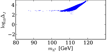
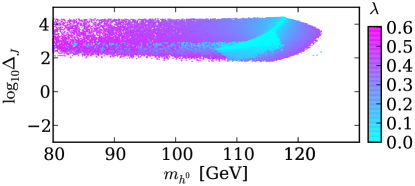
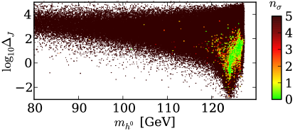
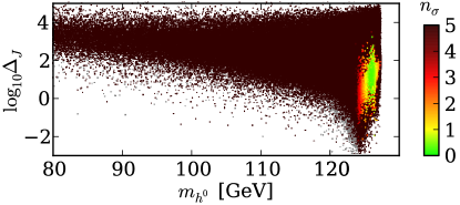
FIG. 5 shows fits to various observables in the framework of the slightly relaxed CNMSSM for fixed values of $A_{0}=-2.5$ TeV and $\tan\beta=10$. For these scans $A_{\lambda}$ and $A_{\kappa}$ are allowed to vary independently from $A_{0}$. We decouple $A_{\lambda}$ and $A_{\kappa}$ from $A_{0}$ to easily obtain a neutralino relic density and a lightest Higgs mass which simultaneously satisfy the experimental constraints. TABLE 1 shows the experimental values of the observables that were used in the fit shown in FIG. 5. The neutralino relic density is required to match the dark matter relic density as measured by Planck Ade:2013ktc . For the lightest Higgs mass we use the PDG combined value PDG:2013 . PDG combined limits are used to constain the sparticle masses, except for the squark and gluino masses; in this case we take the strongest currently listed PDG limits, even though these do not directly apply to the model under consideration, in order to be conservative. The constraints on rare B decays are taken from LHCbAaij:2013aka and HFAGAmhis:2012bh . All constraints are implemented as Gaussian likelihoods except where a limit is indicated, in which case a hard cut is applied.

Table 1: Experimental values of the observables that were used in the fit shown in FIG. 5.

Observable	Experimental value
$\Omega_{DM}h^{2}$	$0.1187\pm 0.0017$ Ade:2013ktc
$m_{h}$	$125.9\pm 0.4$ GeV PDG:2013
$\mathrm{BR}\left(B_{s}\rightarrow\mu^{+}\mu^{-}\right)$	$(2.9\pm 1.1)\times 10^{-9}$ Aaij:2013aka
$\mathrm{BR}\left(b\rightarrow s\gamma\right)$	$(343\pm 21\pm 7)\times 10^{-6}$ Amhis:2012bh
$\mathrm{BR}\left(B\rightarrow\tau\nu\right)$	$(114\pm 22)\times 10^{-6}$ Amhis:2012bh
$m_{\tilde{\chi}^{0}_{1}}$	$>46$ GeV PDG:2013
$m_{\tilde{\chi}^{\pm}_{1}}$	$>94$ GeV if $m_{\tilde{\chi}^{\pm}_{1}}-m_{\tilde{\chi}^{0}_{1}}>3$ GeVPDG:2013
$m_{\tilde{q}}$	$>1.43$ TeV PDG:2013
$m_{\tilde{g}}$	$>1.36$ TeV PDG:2013

The top frame of FIG. 5 is the fit to the relic density alone while the bottom is the two observable combined fit. The statistical significance with which each model point can be rejected is given in units of $\sigma s$. These significances correspond to local p-values, computed assuming the observables’ best fit values are normally distributed with the specified standard deviation. To be conservative, no additional theoretical uncertainty is included in the fit. As the figure shows on the $A_{0}=-2.5$ TeV and $\tan\beta=10$ hypersurface a good fit to both observables can be obtained for the low Jacobian tuning of $\Delta_{J}\sim 1$.

Figure 5: Fits to various observables in the framework of the slightly relaxed CNMSSM for fixed values of $A_{0}=-2.5$ TeV and $\tan\beta=10$. $A_{\lambda}$ and $A_{\kappa}$ are allowed to vary independently from $A_{0}$. TABLE 1 shows the experimental values of the observables that were used in this fit. The top frame is the fit to the relic density alone while the bottom is the two observable combined fit. The statistical significance with which each model point can be rejected is given in units of $\sigma s$. As the figure shows on the $A_{0}=-2.5$ TeV and $\tan\beta=10$ hypersurface a good fit to both observables can be obtained for the low Jacobian tuning of $\Delta_{J}\sim 1$.

IV Conclusions

In this work we presented Bayesian naturalness priors to quantify fine-tuning in the (N)MSSM. These priors emerge automatically during model comparison within the Bayesian evidence.

We compared the Bayesian measure of fine-tuning ($\Delta_{J}$) to the Barbieri-Giudice ($\Delta_{BG}$) and ratio ($\Delta_{EW}$) measures. Even though the Bayesian prior is closely related to the Barbieri-Giudice measure, the numerical value of the Bayesian measure reproduces important features of $\Delta_{EW}$. Both $\Delta_{EW}$ and $\Delta_{J}$ are low in FP scenarios.

Our numerical analysis is limited to fixed ($A_{0},\tan\beta$) slices of the constrained parameter space. For these slices we show that, according to the naturalness prior, the constrained version of the NMSSM is less tuned than the CMSSM. This statement, however, has to be confirmed by comparing Bayesian evidences of the models. The complete parameter space scan and the full Bayesian analysis for the NMSSM is deferred to a later work Monash_Adelaide .

V Acknowledgements

This research was funded in part by the ARC Centre of Excellence for Particle Physics at the Tera-scale, and in part by the Project of Knowledge Innovation Program (PKIP) of Chinese Academy of Sciences Grant No. KJCX2.YW.W10. The use of Monash Sun Grid (MSG) and the Multi-modal Australian ScienceS Imaging and Visualisation Environment (www.MASSIVE.org.au) is also gratefully acknowledged. DK is grateful to Xerxes Tata for the useful discussion. PA thanks Roman Nevzorov and A. G. Williams for helpful comments and discussions during the preparation of this manuscript.

Appendix A Appendix: Jacobian entries

The entries appearing in the Jacobian $J_{\mathcal{T}_{\kappa m_{S}}}$ in Eq. 10 are given in this appendix.

$$a_{1} = -\kappa A_{\kappa}-4\kappa^{2}s-\frac{\lambda A_{\lambda}v^{2}s_{2\beta}}{2s^{2}}\hskip 11.38109pt$$ (15)

$$a_{2} = \lambda\kappa v^{2}\frac{\partial s_{2\beta}}{\partial t_{\beta}}+\frac{\lambda A_{\lambda}v^{2}}{2s}\frac{\partial s_{2\beta}}{\partial t_{\beta}}\hskip 11.38109pt$$ (16)

$$a_{3} = -\frac{\lambda^{2}v^{2}}{M_{Z}^{2}}+\lambda\kappa s_{2\beta}\frac{v^{2}}{M_{Z}^{2}}+\frac{\lambda A_{\lambda}v^{2}s_{2\beta}}{2sM_{Z}^{2}}$$ (17)

$$b_{1} = -\frac{\lambda}{s}\hskip 28.45274ptb_{2}=\frac{1}{2\lambda s^{2}}\frac{2t_{\beta}}{(t_{\beta}^{2}-1)^{2}}(m_{H_{u}}^{2}-m_{H_{d}}^{2})\hskip 28.45274pt$$ (18)

$$b_{3} = -\frac{1}{4\lambda s^{2}}$$ (19)

$$e_{1} = -\frac{2\lambda s\sin{2\beta}-(A_{\lambda}+2\kappa s)}{s^{2}}\hskip 28.45274pt$$ (20)

$$e_{2} = -\frac{1-t_{\beta}^{2}}{t_{\beta}(1+t_{\beta}^{2})}\frac{A_{\lambda}+\kappa s}{s}\hskip 105.2751pt$$ (21)

$$e_{3} = -\frac{\lambda\sin{2\beta}}{\bar{g}^{2}s^{2}}$$ (22)

References

- (1) G. F. Giudice, [arXiv:1307.7879 [hep-ph].
- (2) G. Aad et al. [ATLAS Collaboration], Phys. Lett. B 716, 1 (2012) [arXiv:1207.7214 [hep-ex]].
- (3) S. Chatrchyan et al. [CMS Collaboration], Phys. Lett. B 716, 30 (2012) [arXiv:1207.7235 [hep-ex]].
- (4) S. F. King, M. Mühlleitner, R. Nevzorov and K. Walz, Nucl. Phys. B 870, 323 (2013) [arXiv:1211.5074 [hep-ph]].
- (5) T. Gherghetta, B. von Harling, A. D. Medina and M. A. Schmidt, JHEP 02, 032 (2013) [arXiv:1212.5243 [hep-ph]].
- (6) H. Baer, V. Barger, P. Huang, A. Mustafayev and X. Tata, Phys. Rev. Lett. 109, 161802 (2012) [arXiv:1207.3343 [hep-ph]].
- (7) H. Baer, V. Barger, P. Huang, D. Mickelson, A. Mustafayev and X. Tata, Phys. Rev. D 87, 115028 (2013) [arXiv:1212.2655 [hep-ph]].
- (8) H. Baer, V. Barger and M. Padaffke Kirkland, Phys. Rev. D 88, 055026 (2013) [arXiv:1304.6732 [hep-ph]].
- (9) H. Baer, V. Barger and D. Mickelson, Phys. Rev. D 88, 095013 (2013) [arXiv:1309.2984 [hep-ph]].
- (10) J. R. Ellis, K. Enqvist, D. V. Nanopoulos and F. Zwirner, Mod. Phys. Lett. A 1, 57 (1986).
- (11) R. Barbieri and G. F. Giudice, Nucl. Phys. B 306, 63 (1988)
- (12) G. W. Anderson and D. J. Castano, Phys. Rev. D 52, 1693 (1995) [hep-ph/9412322].
- (13) G. W. Anderson and D. J. Castano, Phys. Lett. B 347, 300 (1995) [hep-ph/9409419].
- (14) P. Athron and D. J. Miller, Phys. Rev. D 76, 075010 (2007) [arXiv:0705.2241 [hep-ph]].
- (15) F. Feroz, M. P. Hobson and M. Bridges, Mon. Not. Roy. Astron. Soc. 398, 1601 (2009) [arXiv:0809.3437 [astro-ph]].
- (16) F. Feroz and M. P. Hobson, Mon. Not. Roy. Astron. Soc. 384, 449 (2008) [arXiv:0704.3704 [astro-ph]].
- (17) B. C. Allanach, K. Cranmer, C. G. Lester and A. M. Weber, JHEP 0708, 023 (2007) [arXiv:0705.0487 [hep-ph]].
- (18) M. E. Cabrera, J. A. Casas and R. Ruiz de Austri JHEP 0903, 075 (2009) [arXiv:0812.0536 [hep-ph]].
- (19) M. E. Cabrera, J. A. Casas and R. Ruiz de Austri JHEP 1005, 043 (2010) [arXiv:0911.4686 [hep-ph]].
- (20) D. M. Ghilencea, H. M. Lee and M. Park, JHEP 1207, 046 (2012) [arXiv:1203.0569 [hep-ph]].
- (21) D. M. Ghilencea and G. G. Ross, Nucl. Phys. B 868, 65 (2013) [arXiv:1208.0837 [hep-ph]].
- (22) D. M. Ghilencea, [arXiv:1311.6144 [hep-ph]].
- (23) S. Fichet, Phys. Rev. D 86, 125029 (2012) [arXiv:1204.4940 [hep-ph]].
- (24) K. Kowalska, S. Munir, L. Roszkowski, E. M. Sessolo, S. Trojanowski and Y. -L. S. Tsai, Phys. Rev. D 87, 115010 (2013) [arXiv:1211.1693 [hep-ph]].
- (25) J. F. Gunion, D. E. Lopez-Fogliani, L. Roszkowski, R. Ruiz de Austri and T. A. Varley, Phys. Rev. D 84 (2011) 055026 [arXiv:1105.1195 [hep-ph]].
- (26) C. Balazs and D. Carter, JHEP 1003 (2010) 016 [AIP Conf. Proc. 1178 (2009) 23] [arXiv:0906.5012 [hep-ph]].
- (27) R. Trotta, F. Feroz, M. P. Hobson, L. Roszkowski and R. Ruiz de Austri, JHEP 0812, 024 (2008) [arXiv:0809.3792 [hep-ph]].
- (28) B. C. Allanach, Comput. Phys. Commun. 143, 305 (2002) [hep-ph/0104145].
- (29) U. Ellwanger and C. Hugonie, Comput. Phys. Commun. 177, 399 (2007) [hep-ph/0612134].
- (30) B.C. Allanach, P. Athron, L. Tunstall, A. Voigt, A. G. Williams, [arXiv:1311.7659 [hep-ph]].
- (31) P. Fayet, Nucl. Phys. B 90, 104 (1975)
- (32) M. Dine, W. Fischler and M. Srednicki, Phys. Lett. B 104, 199 (1981)
- (33) M. Maniatis, Int. J. Mod. Phys. A 25, 3505 (2010) [arXiv:0906.0777 [hep-ph]].
- (34) U. Ellwanger and C. Hugonie and A. M. Teixeira, Phys. Rept. 496, 1 (2010)
- (35) P. Athron, C. Balazs, B. Farmer, E. Hutchison, D. Kim, In preparation.
- (36) J. L. Feng, K. T. Matchev and T. Moroi, Phys. Rev. Lett. 84, 2322 (2000) [hep-ph/9908309].
- (37) J. L. Feng, K. T. Matchev and T. Moroi, Phys. Rev. D 61, 075005 (2000) [hep-ph/9909334].
- (38) J. L. Feng and D. Sanford, Phys. Rev. D 86, 055015 (2012) [arXiv:1205.2372 [hep-ph]].
- (39) J. L. Feng, K. T. Matchev and D. Sanford, Phys. Rev. D 85, 075007 (2012) [arXiv:1112.3021 [hep-ph]].
- (40) A. Djouadi, J. -L. Kneur and G. Moultaka, Comput. Phys. Commun. 176, 426 (2007) [hep-ph/0211331].
- (41) S. F. King, M. Muhlleitner and R. Nevzorov, Nucl. Phys. B 860, 207 (2012) [arXiv:1201.2671 [hep-ph]].
- (42) Planck Collaboration, Astron. & Astrophys. (2014) [arXiv:1303.5062 [astro-ph.CO]].
- (43) Particle Data Group, Phys. Rev. D 86, 010001 (2012) [partial update for 2014 ed.]
- (44) R. Aaij et al. [LHCb Collaboration], Phys. Rev. Lett. 111 (2013) 101805 [arXiv:1307.5024 [hep-ex]].
- (45) Y. Amhis et al. [Heavy Flavor Averaging Group Collaboration], arXiv:1207.1158 [hep-ex]. [online update]