The surface nitrogen abundance of a massive star in relation to its oscillations, rotation, and magnetic field

Abstract

We have composed a sample of 68 massive stars in our galaxy whose projected rotational velocity, effective temperature and gravity are available from high-precision spectroscopic measurements. The additional seven observed variables considered here are their surface nitrogen abundance, rotational frequency, magnetic field strength, and the amplitude and frequency of their dominant acoustic and gravity mode of oscillation. Multiple linear regression to estimate the nitrogen abundance combined with principal components analysis, after addressing the incomplete and truncated nature of the data, reveals that the effective temperature and the frequency of the dominant acoustic oscillation mode are the only two significant predictors for the nitrogen abundance, while the projected rotational velocity and the rotational frequency have no predictive power. The dominant gravity mode and the magnetic field strength are correlated with the effective temperature but have no predictive power for the nitrogen abundance. Our findings are completely based on observations and their proper statistical treatment and call for a new strategy in evaluating the outcome of stellar evolution computations.

1 Introduction

Mixing of chemical species inside stars is poorly understood. Yet, its effect on stellar evolution and supernova explosions, and by implication on the chemical enrichment of galaxies is of prime importance. It was realised already quite some time ago that stellar rotation and the mixing it induces must play a major role in stellar evolution theory (e.g., Herrero et al., 1992) but its inclusion in models is far from trivial, see e.g., Langer (1992); Talon et al. (1997) for early attempts and discussions, while Maeder (2009) is a recent extensive monograph in this topic.

Ways to test the theoretical descriptions used to represent rotational mixing are scarce and are mainly limited to studies of the chemical composition and projected rotational velocity of stellar atmospheres (e.g., Venn & Lambert, 2005; Hunter et al., 2008; Przybilla et al., 2010, among many others). A particularly strong observational diagnostic for mixing is the surface nitrogen abundance of stars that are undergoing hydrogen fusion through the carbon-nitrogen-oxygen cycle in their interior. It turns out that the current theoretical concepts of rotational mixing seemingly fail to explain observations of various massive stars in the Milky Way and in the Magellanic Clouds (Hunter et al., 2008; Brott et al., 2011; Rivero González et al., 2012; Bouret et al., 2012, 2013), leading to intense debates on yet unknown causes of the discrepancies and on the way to identify other physical ingredients lacking in the theoretical models (e.g., Meynet et al., 2011; Potter et al., 2012; Mathis et al., 2013).

Here, we shed new light on the matter by considering a variety of observational data and by subjecting them to careful statistical analysis. In particular, we investigate the relationship between observed stellar oscillations, rotational frequency, magnetic field strength and surface nitrogen abundance in a sample of galactic massive stars for which this multitude of data has recently become available. A direct comparison between observed rotational properties with evolutionary models would ideally be based on a value for the equatorial rotation velocity. This would require having either precise measurements of both the rotational frequency and the stellar radius, or else of the inclination angle $i$ between the rotational axis of the star and the line-of-sight of the observer, in addition to $v\sin\,i$. While the combination $(v\sin\,i,i)$ is available for some pulsating stars from an analysis of time-series spectroscopy and for a few magnetic stars from spectro-polarimetry, this concerns very few stars. Similarly, direct measurements of the radii are in general not available for massive stars. Hence, a specific point of attention in this work is whether the use of the rotational frequency, rather than the projected rotational velocity, leads to an improved diagnostic.

2 Sample Selection

Figure 1: A ($\log\,T_{\rm eff},\log\,g$) diagram of the measured stars (squares for single stars, triangles for spectroscopic binaries) and of evolutionary tracks (full lines, see text) for masses of 3, 4, 5, 7, 10, 15, 20, 30, 40 M_⊙, from right to left. A typical error box is indicated in the upper left corner.

Sample selection was restricted to stars whose effective temperature, gravity and projected rotational velocity are available from high signal-to-noise high-resolution spectroscopy. From this sample, we kept the stars for which at most one of the following four additional properties has missing data: nitrogen abundance, rotational frequency, magnetic field strength, and oscillations. This rather strict criterion of missingness was adopted to achieve a good starting point for the statistical analysis outlined in the following section and implied that only Galactic OB stars were retained in the sample.

Regarding the oscillations detected, we considered the frequency and the amplitude of the dominant acoustic mode and of the dominant gravity mode of the star (see Aerts et al., 2010, for a definition and extensive description of such heat-driven oscillations in massive stars) whenever available in the literature. We downloaded the Hipparcos data from Perryman (1997) and derived upper limits for the oscillation amplitudes as four times the standard deviation of these data. These upper limits were adopted in the case of stars for which one or both types of oscillations have not yet been detected.

The magnetic field strength under the assumption of an oblique dipole configuration is either available as a measured value (in case a time series of spectro-polarimetry was observed) or as a lower limit (because the projection factor between the line-of-sight and the magnetic axis at the time of measurement is unknown). We adopted the most recent published results derived from high-resolution polarimeters such as ESPaDOnS, NARVAL or HARPSpol (data sources are listed along with the data in Table 3). In absence of those, we took results based on the lower-resolution spectrographs such as, e.g., FORS1/2. For a comparison between the interpretations based on these two types of measurements, we refer to Shultz et al. (2012). We added to those data all unpublished null detections obtained by the MiMeS (Magnetism in Massive Stars) collaboration.

The rotational frequency was deduced from time series of spectro-polarimetric data or from rotational splitting of oscillation frequencies. It is noteworthy that, whenever values from these two independent methods are available for a star, they are in excellent agreement (see Briquet et al., 2013, for a recent example). Whenever available, we took the $v\sin\,i$-values deduced from time-series spectroscopy analysed in such a way that line-broadening due to the oscillations was carefully taken into account (e.g., Aerts & De Cat, 2003; Aerts et al., 2010, Chapter 6). In the absence of time-series spectroscopy or spectro-polarimetry, we relied on the $v\sin\,i$-values derived from high-resolution single snapshot spectra.

For the values of $\log\,T_{\rm eff}$, $\log\,g$, and the nitrogen abundance, various sources are available in the literature, based on different methods and analysis codes. We relied on recent NLTE analyses of high-resolution high signal-to-noise spectroscopy, mostly done by Nieva & Przybilla (2012); Martins et al. (2012a, b); Morel et al. (2008), as well as on detailed asteroseismic or spectro-polarimetric studies of individual targets which also included NLTE line-fitting of the high-precision spectroscopy. For stars not covered in this way, we took the most recent high-precision spectroscopic data source available.

Table 1 gives a summary of the observed properties of the 68 sample stars, with an indication of the level of completeness of the sampling for each of the ten variables $X_{1},\ldots,X_{10}$, while Table 3 contains the actual data of all stars we used in our analyses along with all the data sources. All stars are plotted in a $(\log\,T_{\rm eff},\log\,g)$ diagram in Fig. 1, together with some evolutionary tracks starting from the zero-age main-sequence. These were computed with the MESA stellar evolution code (Paxton et al., 2011, 2013), taking the solar composition given by Asplund et al. (2009) and ignoring rotational mixing. We adopted the mixing-length theory of convection with a mixing-length value of 1.8 local pressure scale heights. The Schwarzschild criterion for convection was used, along with a fully-mixed core overshoot region extending over 0.15 local pressure scale heights, which is a good average of all seismically determined values for OB pulsators (Aerts, 2014). Among the 68 stars are 17 unevolved spectroscopic binaries whose orbits are known and for which the binarity has appropriately been taken into account in the primary’s parameters listed in Table 3. These are indicated with triangles in Fig. 1.

Some comments on Fig. 1 are warranted. Hubrig et al. (2006) already pointed out the high $\log\,g$ value with large uncertainty for the star HD 46005, placing it below the ZAMS. On the other side of low $\log\,g$ values, we see that only one star in the sample is evolved beyond core-hydrogen burning. This is the rotational variable B5II star HD 46769 studied from time-resolved CoRoT space photometry and high-precision spectroscopy (Aerts et al., 2013a). The additional seemingly evolved object is the double-lined spectroscopic eclipsing binary V380 Cyg, for which a core overshoot value of 0.6 local pressure scale heights was reported to bring the model-independent measured dynamical mass deduced for the primary in agreement with single-star evolutionary models (Guinan et al., 2000). This binary is the brightest star observed by the Kepler spacecraft and these high-precision photometric space data along with an extensive new set of time-resolved high-resolution spectroscopy led to dynamical masses with a relative precision near 1% and revealed the primary to be a low-amplitude rotational variable with mild silicon spots and additional stochastic low-frequency photometric variability. These latest data confirmed the earlier findings that a high core-overshoot parameter is necessary to bring the primary’s mass into agreement with single-star models and that the secondary does not fit the isochrones for the measured equatorial rotational velocity and metallicity of both stars (Tkachenko et al., 2013). This binary indicates that the current stellar models have too limited near-core mixing. As can further be seen in Fig. 1, all other stars in our sample cover the main-sequence phase of evolution.

Finally, the missing data due to lack of measurements were assumed to be missing at random (Rubin, 1976; Molenberghs & Kenward, 2007), in line with common statistical practice. As is often done in astronomy, we consider logarithmic quantities for the variables $X_{4}$, $X_{6}$, $X_{7}$, $X_{8}$, $X_{9}$, and $X_{10}$, given their wide ranges of possible values among OB stars, where $X_{7}$ was transformed in such a way that a null detection for the magnetic field translates into zero value.

Table 1: Characteristics of the observed data set.

Variable	Quantity	Physical meaning	Unit	Observed range	Tr?	% obs.
$X_{1}$	$v\sin i$	projected rotational velocity	km/s	[0,310]	no	100%
$X_{2}$	$f_{\rm rot}$	rotational frequency	per day	[0,2.505]	no	94%
$X_{3}$	$f_{g}$	gravity mode frequency	per day	[0.039,1.157]	no	32%
$X_{4}$	$A_{g}$	amplitude of $f_{g}$	mmag	[0.11,24.90]	yes	96%
$X_{5}$	$f_{p}$	acoustic mode frequency	per day	[3.258,10.935]	no	32%
$X_{6}$	$A_{p}$	amplitude of $f_{p}$	mmag	[0.05,38.10]	yes	96%
$X_{7}$	$\log(1+B_{\rm pol})$	magnetic field strength	Gauss	[0.00,4.20]	yes	96%
$X_{8}$	$\log T_{\rm eff}$	effective temperature	Kelvin	[4.061,4.633]	no	100%
$X_{9}$	$\log g$	gravity	cm/s2	[2.70,4.43]	no	100%
$X_{10}$	$12+\log[N/H]$	nitrogen abundance	dex	[7.42,8.95]	yes	59%

3 Statistical Methodology and Analysis

Handling the incomplete and truncated data was done by multiple imputation combined with acceptance-rejection sampling (Rubin, 1987; Schafer, 1997; Little & Rubin, 2002; Carpenter & Kenward, 2013). These are established techniques in medical statistics but less so in astrophysics. We thus explain first why we used that methodology and how we tuned it to our application before outlining the various steps involved in the analysis.

The great strength of multiple imputation is that it is a principled statistical method that takes proper account of the loss of information in the incomplete data. As with any statistical technique it does of course rest on assumptions. The role of these assumptions becomes more critical with increasing amounts of missing information. However, the connection between missing information and the amount of missing data is far from straightforward. For example, missing information also depends on the type of outcome variables, the patterns of missingness, and the dependence structure between what is observed and what is missing, and the model fitted. For these reasons, we have limited the data set to the variables listed in Table 1, where the poorest level of completeness occurs for the oscillation frequencies ($X_{3}$ and $X_{5}$, which each have a coverage of 32%) but we have well-determined upper limits for their amplitudes from the Hipparcos data ($X_{4}$ and $X_{6}$).

Because data come from various sources, there is heterogeneity in the error with which they are measured. Moreover, it is well known that good error propagation for spectroscopic quantities ($X_{1}$, $X_{7}$, $X_{8}$, $X_{9}$, $X_{10}$) is a difficult problem due to the possible dominance of systematic uncertainties over statistical errors. These systematic uncertainties result from a combination of instrument calibrations, varying atmospheric conditions, spectrum normalization uncertainties, and limitations in the theory of spectral line predictions. Given that our analysis is based on multiple regression, in which one works conditionally on the values observed for the explanatory variables, such heterogeneity is not explicitly accommodated. The implication of this is that estimated relationships may be somewhat attenuated (Carroll et al., 2010), but the logic of the analysis is not undermined. In particular, ignorance of the measurement errors will not create artefacts such as non-existing relationships.

3.1 Incomplete Data: Missingness and Truncation

Let $\mbox{\boldmath$X$}_{i}=(X_{i1},\dots,X_{ip})^{T}$ be the column vector of $p$ measurements for star $i=1,\dots,n$. The data are commonly organized in a dataset $\mbox{\boldmath$X$}=(\mbox{\boldmath$X$}_{1}^{T},\dots,\mbox{\boldmath$X$}_{n}^{T})^{T}$ that takes the form of a rectangular matrix of dimension $n\times p$. When the data are complete, a wide variety of statistical models can be fitted to them. As an example, consider a regression model

$$X_{i1}=\beta_{1}+\beta_{2}X_{i2}+\cdots+\beta_{p}X_{ip}+\varepsilon_{i},$$ (1)

where $\mbox{\boldmath$\beta$}=(\beta_{1},\dots,\beta_{p})^{T}$ is a vector of unknown regression coefficients and the error term $\varepsilon_{i}$ is assumed to follow a distribution with mean zero and variance $\sigma^{2}$. Using conventional methodology and standard statistical software, the parameters $\beta$ and $\sigma^{2}$ can then be estimated, along with measures of precision, i.e., confidence intervals.

In the current problem, we are faced with two types of incompleteness. First, some values $X_{ij}$ are entirely missing. Second, for some values $X_{ij}$ bounds are available per individual star, but not the actual value, i.e., the information is restricted to $\ell_{ij}\leq X_{ij}\leq u_{ij}$, with $\ell_{ij}$ ($u_{ij}$) a star-specific lower bound (upper bound). Note that, if only one bound is available for all stars simultaneously, then we use an additional superscript $r$ to indicate that, i.e., either $\ell_{ij}=\ell^{r}_{ij}$ for one lower bound only or $u_{ij}=u^{r}_{ij}$ for one upper bound only, where $[\ell^{r}_{ij},u^{r}_{ij}]$ is then the total range of the random variable $X_{ij}$. This occurs, e.g., due to the requirement for positive frequency values, leading to zero as lower bound for all stars for variables $X_{2}$, $X_{3}$, and $X_{5}$. Similarly, we required the values for $X_{10}$ to be bound by physically meaningful values as explained in the following section. In summary, it is possible to unify missingness and truncation by simultaneously setting both bounds to their range limits. Even a properly observed value can be placed within this setting: $\ell_{ij}=X_{ij}=u_{ij}$. Thus, the vectors $\mbox{\boldmath$\ell$}_{i}$, and $\mbox{\boldmath$u$}_{i}$ fully describe the data available on star $i$.

Modeling such data has received a large amount of attention. Here, we opted for so-called multiple imputation (Rubin, 1987; Schafer, 1997; Little & Rubin, 2002; Carpenter & Kenward, 2013) combined with acceptance-rejection sampling. Multiple imputation consists of three steps. In the first or imputation step, the principle is to replace each missing values with $M$ copies or so-called imputations. These are drawn from the predictive distribution of what is missing, given what is observed. Because values are drawn multiple times, rather than filled in once, the phenomenon that incomplete data lead to reduced statistical information is maintained, in contrast to single imputation. Let us write the model to be fitted symbolically as

$$f(\mbox{\boldmath$x$}_{i}|\mbox{\boldmath$\theta$}),$$ (2)

where $\mbox{\boldmath$x$}_{i}$ is the realized value of $\mbox{\boldmath$X$}_{i}$ and $\theta$ groups all model parameters. The modeler thus obtains $M$ completed datasets. In the second or modeling step, each of these is analyzed separately, as if the data were complete. Thus, $M$ estimates of $\theta$, are obtained. We denote these by $\widehat{\mbox{\boldmath$\theta$}}_{m}$, with $m=1,\dots,M$. The same is true for the corresponding measures of precision. Let the estimated variance-covariance matrix for $\widehat{\mbox{\boldmath$\theta$}}_{m}$ be $\widehat{U}_{m}$. In the third or analysis step, these $M$ estimates are combined into a single set of parameter and precision estimates, using Rubin’s rules (Rubin, 1987; Schafer, 1997; Little & Rubin, 2002; Carpenter & Kenward, 2013):

$$\widehat{\mbox{\boldmath$\theta$}} = \frac{1}{M}\sum_{m=1}^{M}\widehat{\mbox{\boldmath$\theta$}}_{m},$$ (3)

$$\widehat{U} = \frac{1}{M}\sum_{m=1}^{M}U_{m}+\frac{M+1}{M(M-1)}\sum_{m=1}^{M}(\widehat{\mbox{\boldmath$\theta$}}_{m}-\widehat{\mbox{\boldmath$\theta$}})(\widehat{\mbox{\boldmath$\theta$}}_{m}-\widehat{\mbox{\boldmath$\theta$}})^{T}.$$ (4)

Step 2 requires fitting a model to a complete set of data, and to repeat this exercise $M$ times; in step 3, Rubin’s rules (3)–(4) are applied. The most involved step is the first one. We turn to it next.

For our purposes in particular, the constraints make the use of multiple imputation non standard, in contrast to when the only complication is missingness. Consider for our purposes the general setting where $\mbox{\boldmath$X$}_{i}$ is a vector with three sub-vectors $\mbox{\boldmath$X$}_{i}=(\mbox{\boldmath$X$}_{i1}^{T},\mbox{\boldmath$X$}_{i2}^{T},\mbox{\boldmath$X$}_{i3}^{T})^{T}$, where the notation implies that we first transpose the individual sub-vectors from column to row, place them all next to each other, and then turn it into a column once again, in such a way that $\mbox{\boldmath$X$}_{i1}$ is observed, $\mbox{\boldmath$X$}_{i2}$ is truncated with conditions $\mbox{\boldmath$C$}_{i2}=\mbox{\boldmath$\ell$}_{i2}\leq\mbox{\boldmath$X$}_{i2}\leq\mbox{\boldmath$u$}_{i2}$, and $\mbox{\boldmath$X$}_{i3}$ is fully missing. Sampling is then needed from

$$f(\mbox{\boldmath$x$}_{i2},\mbox{\boldmath$x$}_{i3}|\mbox{\boldmath$x$}_{i1},\mbox{\boldmath$c$}_{i2},\mbox{\boldmath$\theta$})=f(\mbox{\boldmath$x$}_{i2},\mbox{\boldmath$x$}_{i3}|\mbox{\boldmath$x$}_{i1},\mbox{\boldmath$\theta$})\cdot\frac{1}{f(\mbox{\boldmath$c$}_{i2}|\mbox{\boldmath$x$}_{i1},\mbox{\boldmath$\theta$})}.$$ (5)

By contrast, should $\mbox{\boldmath$X$}_{i2}$ as well as $\mbox{\boldmath$X$}_{i3}$ be fully unobserved, then it would be sufficient to sample from $f(\mbox{\boldmath$x$}_{i2},\mbox{\boldmath$x$}_{i3}|\mbox{\boldmath$x$}_{i1},\mbox{\boldmath$\theta$})$, the first factor of Eq. (5).

Assuming a multivariate normal distribution for the variables in the imputation model implies that every conditional distribution of one subset given another is still multivariate normal (Johnson & Wichern, 2000; Carpenter & Kenward, 2013, Appendix B). Hence, relying on this convenient property, the conditional density is also multivariate normal and takes the following form:

$$f(\mbox{\boldmath$x$}_{i2},\mbox{\boldmath$x$}_{i3}|\mbox{\boldmath$x$}_{i1},\mbox{\boldmath$\theta$})=\phi_{p_{2}+p_{3}}\left(\mbox{\boldmath$x$}_{i,23}\left|\mbox{\boldmath$\mu$}_{23}+\Sigma_{23,1}\Sigma_{1,1}^{-1}(\mbox{\boldmath$x$}_{i1}-\mbox{\boldmath$\mu$}_{1});\Sigma_{23,23}-\Sigma_{23,1}\Sigma_{1,1}^{-1}\Sigma_{1,23}\right.\right),$$ (6)

where $\phi_{p_{2}+p_{3}}(\cdot;\cdot)$ is the multivariate normal density with dimension $p_{2}+p_{3}$. In this notation, an index ‘23’ indicates selection of the appropriate components of the full vector or matrix pertaining to the second and third sub-vector combined. Not only is this predictive distribution much simpler than Eq. (5), expressions of this form are part of standard implementations of multiple imputation (Carpenter & Kenward, 2013).

The above considerations suggest combining multiple imputation with so-called acceptance-rejection sampling (von Neumann, 1951; Gilks et al., 1996; Robert & Casella, 2004). Generally, when sampling from $h(\mbox{\boldmath$x$})$ is required, but sampling from $g(\mbox{\boldmath$x$})$ is much easier, then one can proceed by sampling from the latter density, provided that there is a value $M>1$ such that $h(\mbox{\boldmath$x$})/g(\mbox{\boldmath$x$})\leq M$. In our case, $h(\mbox{\boldmath$x$}_{i})=f(\mbox{\boldmath$x$}_{i2},\mbox{\boldmath$x$}_{i3}|\mbox{\boldmath$x$}_{i1},\mbox{\boldmath$c$}_{i2},\mbox{\boldmath$\theta$})$ while $g(\mbox{\boldmath$x$}_{i})=f(\mbox{\boldmath$x$}_{i2},\mbox{\boldmath$x$}_{i3}|\mbox{\boldmath$x$}_{i1},\mbox{\boldmath$\theta$})$, and the ratio between both is $M=f(\mbox{\boldmath$c$}_{i2}|\mbox{\boldmath$x$}_{i1},\mbox{\boldmath$\theta$})^{-1}\geq 1$.

Acceptance-rejection sampling operates in the following way. Draw $X$ from $g(\mbox{\boldmath$x$})$ and $U\sim U(0,1)$, a uniform variable on the unit interval. Then, accept the draw if $U\leq h(\mbox{\boldmath$x$})/[Mg(\mbox{\boldmath$x$})]$ and reject it otherwise. Given the form of Eq. (5), $h(\mbox{\boldmath$x$})/[Mg(\mbox{\boldmath$x$})]=1$ when $\mbox{\boldmath$C$}_{i2}$ is satisfied and 0 otherwise. Hence, thanks to the special situation posed by truncation, every draw that satisfies the constraint is always accepted, otherwise, it is always rejected.

Thus, in practice, multiple imputations are drawn from a multivariate distribution assuming that the missing values and the truncated values are all missing, but draws are accepted only if they satisfy the constraints $\mbox{\boldmath$C$}_{i2}$. The draws that are accepted then form the appropriate predictive distribution. Acceptance-rejection sampling can be very inefficient when $g(\cdot)$ and $h(\cdot)$ are very different, resulting in small proportions of acceptable draws. To improve the efficiency of our imputation procedure, we have additionally used transformations that automatically respect range restrictions whenever such restrictions are applicable to a variable for all stars simultaneously, rather than to values for some particular stars only. For example, an additional square root transformation was adopted to ensure non-negativity.

3.2 Principal Components

Principal component analysis (Krzanowski, 1988; Johnson & Wichern, 2000), abbreviated as PCA, is a classical exploratory method, based on rotating outcome vectors $\mbox{\boldmath$Y$}_{i}=L\mbox{\boldmath$X$}_{i}$ with the requirement that the components of the transformed vectors are uncorrelated, that the first one has maximal variance, the second one maximal variance given the first, etc. Ordinarily, PCA is conducted on standardized, hence unitless, input variables $\mbox{\boldmath$X$}_{i}$. Technically, the transformation matrix $L$ is the set of eigenvectors of the correlation matrix of the input variables $\mbox{\boldmath$X$}_{i}$. The variances of the transformed variables are found as the eigenvalues of the said correlation matrix. For example, the first principal component

$$Y_{i1}=\ell_{11}X_{i1}+\dots+\ell_{1p}X_{ip}$$ (7)

is determined by the first eigenvector $\mbox{\boldmath$\ell$}_{1}=(\ell_{11},\dots,\ell_{1p})^{T}$ and its variance is $\lambda_{1}$, the leading eigenvalue. The coefficients of $\mbox{\boldmath$\ell$}_{1}$ indicate the importance with which the observed variables $X_{ij}$ contribute to the first principal component, with the same logic applying to the other principal components. Further, $\lambda_{1}/p$ is the fraction of the total variance in the original, standardized variables that is captured by the first principal components.

3.3 Application to the Selected Sample

For our application, variables $X_{1}$, $X_{8}$, and $X_{9}$ ($v\sin\,i$, $\log\,T_{\rm eff}$, and $\log\,g$) are observed for all 68 stars, while all others have missing values (see Table 1). By definition, all variables must be positive and are thus truncated at zero as their lower limit, but we use the measured lower limits for $X_{7}$ (the magnetic field strength) when available. Furthermore, there is truncation as an upper limit on variables $X_{4}$, $X_{6}$, and $X_{10}$ (the oscillation mode amplitudes and the nitrogen abundance). For $X_{10}$, we required physically meaningful results in that imputed values must be contained in $[6.8,9.0]$ following results achieved for the Milky Way and the Magellanic Clouds (Trundle et al., 2007; Rivero González et al., 2012).

We fit a linear regression model to the nitrogen abundance ($X_{10}$), with $X_{1}$, $X_{2}$, $X_{3}$, $X_{4}$, $X_{5}$, $X_{6}$, $X_{7}$, $X_{8}$, and $X_{9}$ as potential predictors. Although obviously from a physical perspective a linear model does not necessarily reflect the underlying theory, it does have specific advantages that are appropriate in this setting. First, a linear regression does not rest on a priori theory and hence is neutral with respect to the specific relationships uncovered. Second, it is not the aim to establish an entire physical theory for the processes being modelled, but rather to bring to light important relationships that would be hard to unravel when considering only one variate at a time and that can then be explored further.

Twenty imputations were drawn, using the Monte Carlo Markov Chain method (Neter et al., 1996). The advantage of this method is that it can easily handle missingness of a non-monotone type, i.e., where arbitrary patterns of missingness occur among the stars. It is well-known that small numbers of imputations typically produce valid results, and Little & Rubin (2002) even quote five as sufficient choice. This is relevant for very large data bases, where drawing imputations is computationally costly, while here the number of imputations is not really of concern, given that there are only 68 stars. On the other hand, acceptance-rejection sampling with bounds applying to the variables, necessitates drawing large numbers of imputations. For some stars, 5,000 imputations were needed to obtain the requested number of 20 non-rejected imputations. Even then, for 4 of the 68 stars, no valid draws could be found. These stars are indicated in Table 3. A sensitivity analysis was conducted to address this issue (see Section 3.4), as is common practice in statistical modeling.

A regression model was then fitted to the data by first fitting it to all 20 imputations and then combining the results using the rules outlined in Section 3.1. To select a well-fitting, parsimonious model, two routes were followed. In the first, backward selection (Neter et al., 1996), all nine predictor variables were included. Then, the least significant one was deleted, the model re-fitted, and the process repeated until only significant predictors remained. Significance is defined at the conventional five percent level (indicated as $p<0.05$). It turns out that only two predictors ($X_{5}$ and $X_{8}$, i.e., $f_{p}$ and $\log\,T_{\rm eff}$) are significant (top part of Table 2). In the second, forward selection starts from including only the most significant predictor at first, which is $X_{8}$ as can be seen from the top left-hand columns in Table 2. Thereafter, the model is re-fitted with $X_{8}$ included by default, paired with each one of the remaining predictors in turn. The most significant of these is again $X_{5}$. The process was iterated but no further significant predictors could be added. While generally backward and forward selection can lead to very different models, here the same two predictors for the nitrogen abundance ($X_{10}$) are selected with both approaches, i.e., the effective temperature ($X_{8}$) and the frequency of the dominant acoustic oscillation mode ($X_{5}$). The top part of Table 2 describes the results of the model selection processes.

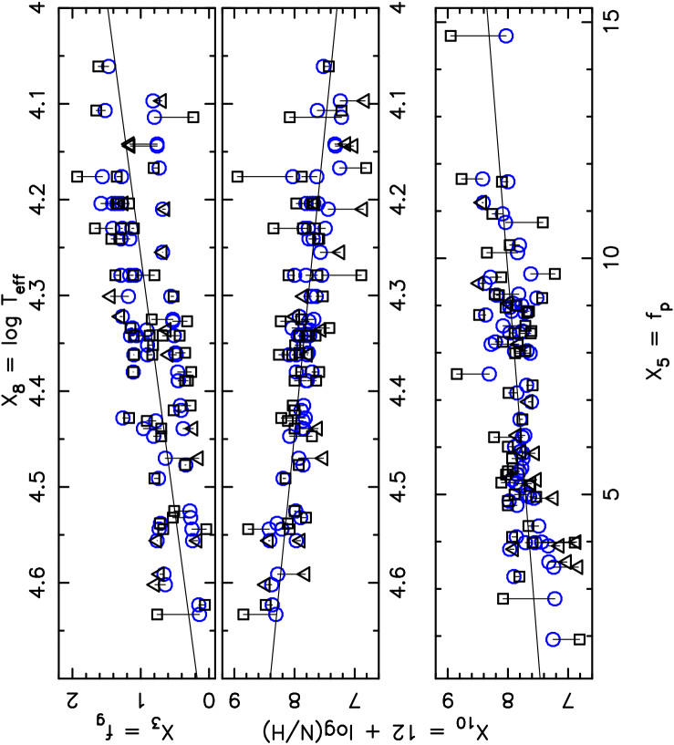
Figure 2: Observed or averaged imputed values (squares for single stars, triangles for spectroscopic binaries) connected by lines to the values predicted by the joint models described in Table 2 (circles, blue in the online version of the paper) for the gravity-mode frequency ($X_{3}$, upper panel) and for the nitrogen abundance ($X_{10}$, lower two panels). The full lines represent the univariate model fits listed in the left part of Table 2.

Figure 3: Observed or averaged imputed values (squares for single stars, triangles for spectroscopic binaries) for the nitrogen abundance ($X_{10}$) as a function of $v\sin\,i$ and the rotation frequency ($X_{1}$ and $X_{2}$).

Returning to the left-hand side of Table 2, these are the coefficients (with standard errors in brackets), and significance levels when the two predictors are considered one at a time. Qualitatively, $X_{5}$, i.e., the frequency of the dominant acoustic mode, is a significant predictor on its own for the nitrogen abundance ($X_{10}$). The fraction of the variance explained by the model (denoted as $R^{2}$) for this single predictor ranges up to 36% for the nitrogen abundance. The effective temperature ($X_{8}$) explains up to 37% of the variance of $X_{10}$ and is also a significant predictor on its own.

The lower two panels of Figure 2 present an illustration of the quality of the joint model. The observed or averaged imputed values of $X_{10}$ (squares for single stars, triangles for spectroscopic binaries) are connected with those predicted by the joint model for $X_{10}$ given in the upper part of Table 2 (circles), as a function of $X_{8}$ (middle panel) and of $X_{5}$ (lower panel). Although the joint model is satisfactory, the corresponding fraction of the variance explained by the model across the 20 imputations is at best 54%.

The results of our statistical modeling lead to the following hypotheses. The acoustic mode frequencies are a measure of the mean density of the star (e.g., Aerts et al., 2010). Following the mass-radius relation that holds during core-hydrogen burning, the acoustic frequencies decrease as the mass of the star increases. On the other hand, the effective temperature increases as the mass increases. From the coefficients of the joint model for the nitrogen abundance in Table 2 and the range of values for $X_{5}$ and $X_{8}$ as given in Table 1, we find that the effect of the temperature is dominant over the one of the acoustic mode. Thus, among the sample of OB stars considered here, the higher-mass O stars have more nitrogen enrichment than the lower-mass B stars, as also found in the study by Rivero González et al. (2012), but the presence of acoustic modes further seems to increase the nitrogen abundance and this increase due to the oscillations gets larger as we move from the early O stars to the late B stars.

To investigate inter-relationships among the variables as well as the variance in the data set as a whole, without focusing solely on the nitrogen abundance, we performed a principal component analysis (Krzanowski, 1988; Johnson & Wichern, 2000), as discussed in Section 3.2. This revealed evidence of two relationships: a first one between the dominant gravity-mode frequency ($X_{3}$), the magnetic field strength ($X_{7}$), the effective temperature ($X_{8}$), and the rotational variables ($X_{1}$ and $X_{2}$) explaining 29% of the variance in the data set and a second one between the nitrogen abundance ($X_{10}$), some of the mode properties ($X_{4}$, $X_{5}$) and the effective temperature ($X_{8}$) explaining 19% of the variance. It is reassuring that the joint model for the nitrogen abundance is recovered in this way from the second principal component. Following the first principal component, a joint model analysis was repeated for variable $X_{3}$ ($f_{g}$) and led to the results in bottom part of Table 2: the lower the effective temperature and the stronger the magnetic field, the higher the gravity-mode frequency, while the rotational frequency and projected rotational velocity were found to be insignificant as predictors for $X_{3}$.

The upper panel of Figure 2 is an illustration of the quality of this joint model for $X_{3}$. Again, the observed or averaged imputed values of $X_{3}$ are connected to those predicted by the joint model given in the lower part of Table 2 (circles), as a function of $X_{8}$. In this case, the joint model across the 20 imputations explains up to 65% of the variance in the frequency of the dominant gravity mode. The increase of the gravity-mode frequencies with decrease of the effective temperature was already reported by De Cat & Aerts (2002, their Fig. 18) from their much smaller sample of slowly pulsating B stars, which covers only a very narrow range in effective temperature compared to the sample we composed here. In addition, we find a correlation between the gravity-mode frequency and the magnetic field strength. As far as we are aware, such a connection has not been reported before from observational diagnostics, although tight relationships between low-frequency gravity modes and the magnetic field strength have been presented in theoretical work (e.g., Hermans et al., 1990). Of course, we must keep in mind that the spectro-polarimetric measurements upon which we relied in this work reveal only the topology and strength of the magnetic field in the outer layers of the star while the internal properties may be quite different. Moreover, the relationship we find results directly from the imputed values of the magnetic field strength and gravity-mode frequency. Indeed, it cannot be revealed without imputation, because very few stars with both gravity-mode oscillations and a positive magnetic field strength have been detected. In our sample, e.g., 20 stars have both magnetic field measurements and detected gravity modes, but for 18 of those a null detection for the magnetic field strength occurs. Hence few gravity-mode oscillators have a magnetic field, but the imputed values for $X_{7}$ for all stars suggest a correlation between $X_{3}$ and $X_{7}$ which remains to be checked in the future from new magnetic gravity-mode pulsators yet to be discovered.

3.4 Sensitivity Analysis

The fact that four stars were removed from the joint analyses out of necessity needs to be addressed. We performed a so-called sensitivity analysis by also considering multiple imputation and acceptance-rejection without requiring zero lower bounds and without transforming the data to their square-root value. This allowed all 68 stars to be included and led to very similar results, although the frequency of rotation ($X_{2}$) or of the gravity mode ($X_{3}$) for some of these stars were assigned negative imputed values.

Table 2: Parameter estimates (standard errors), $p$-values, and the fraction of the variance explained by the model $(R^{2})$.

		Separate models				Joint model
Pred.		Estimate (s.e.)	$p$	$R^{2}$ range		Estimate (s.e.)	$p$	$R^{2}$ range
Models for $X_{10}$
intercept		—	—	—		0.6744(1.9285)	—
$X_{5}$		0.0622(0.0225)	0.0068	[0.05;0.36]		0.0595(0.0217)	0.0079
$X_{8}$		1.5848(0.5009)	0.0018	[0.08;0.37]		1.5515(0.4428)	0.0006
								[0.21;0.54]
Models for $X_{3}$
intercept		—	—	—		6.0323(2.2180)	—
$X_{7}$		0.1801(0.0412)	$<$0.0001	[0.26;0.56]		0.1546(0.0386)	0.0001
$X_{8}$		-1.8711(0.5888)	0.0018	[0.11;0.31]		-1.2723(0.5087)	0.0136
								[0.34;0.65]

4 Discussion

The theory of single-star evolution relying on rotational mixing predicts that the surface nitrogen abundance of a star ($X_{10}$) should strongly depend on its equatorial rotation velocity. Hence, recent observational studies aimed to test the theoretical predictions mainly considered the observed projected rotational velocity ($X_{1}$) and corrected it by assuming equal probability of all possible inclination angles to take away the dependence on the unknown factor $\sin\,i$ (e.g., Hunter et al., 2008; Brott et al., 2011; Rivero González et al., 2012; Bouret et al., 2012, 2013). Those studies led to the conclusion that the theoretical models fail to explain the observed values of the nitrogen abundance. Here, we come to a similar conclusion, by relying on a multitude of observed stellar properties of 64 galactic OB stars. In particular, our sample contains a majority of stars with $v\sin\,i$ below 100 km s^-1 while their nitrogen abundance ranges from about 7 to almost 9 dex. We deduce that neither the projected rotational velocity ($X_{1}$) nor the rotational frequency ($X_{2}$) has predictive power for the measured nitrogen abundance. This is illustrated graphically in Fig. 3. Comparison of the middle and lower panels of Fig. 2 and both panels of Fig. 3 visually shows that the rotational parameters are indeed less suitable as predictors of the nitrogen abundance compared to the effective temperature and the dominant acoustic oscillation mode frequency.

In fact, our results imply that none of the nine variables considered here is by itself able to predict more than a third of the variance in the nitrogen abundance. The joint bivariate model developed for the nitrogen abundance listed in Table 2, i.e.,

$$12+\log[N/H]=0.6744(1.9285)+0.0595(0.0217)\cdot f_{p}+1.5515(0.4428)\cdot\log\,T_{\rm eff}$$ (8)

offers an appropriate yet still incomplete comparison between theory and observations, for the range of stellar parameters in the considered galactic sample.

We come to the conclusion that mixing must occur already early-on in the core-hydrogen burning phase for a considerable fraction of massive stars and that it cannot be due to rotational mixing alone. The same conclusion was reached by an independent study of LMC O stars by Rivero González et al. (2012). Other dynamical phenomena causing mixing must thus be considered. From the statistical modeling based on the observed quantities treated in this work, heat-driven oscillation mode frequencies are a more suitable predictor for mixing compared to the magnetic field strength and the rotation in the sample of stars we studied here. Hence we suggest to include the oscillation properties into future evaluations of theoretical model predictions, e.g., by means of Eq.(8), rather than or in addition to the rotational properties.

Whether our conclusions hold for evolved massive stars and/or for metal-poor stars cannot be checked at present, because the asteroseismic data needed for such a study is lacking. Unfortunately, relatively few massive stars have been monitored sufficiently long in high-precision space photometry because such objects hardly occurred in the fields-of-view of the CoRoT and Kepler space missions, given that these satellites focused on exoplanet hunting around faint cool stars in rather crowded fields, for which the presence of bright massive stars is a nuissance. It will thus require large dedicated and coordinated ground-based efforts to remedy this situation, because long-term monitoring is necessary to reveal and unravel the oscillation properties of evolved OB stars. The potential of such studies from space photometry is clear and it could be tackled with the Kepler2.0 mission concept (see, e.g., Aerts et al., 2013b) and with the future PLATO2.0 mission (Rauer et al., 2013).

Apart from the observed acoustic and gravity modes excited by a heat-mechanism in the stellar envelope upon which we relied in this work, large-scale low-frequency internal gravity waves excited by the convective core, as in the studies by Browning et al. (2004); Neiner et al. (2012b); Rogers et al. (2013); Mathis et al. (2013), may contribute considerably to the surface nitrogen abundance if these waves are able to propagate through the acoustic mode cavity and to transport chemical species in addition to angular momentum. So far, theoretical or simulation studies focused on the angular momentum transport of such internal gravity waves but it should be well possible to extend those studies to the chemical transport they may induce. The frequency spectrum of internal gravity waves computed from 2D simulations for a 3 M_⊙ star by Rogers et al. (2013) coincides with the frequency range of running waves expected for OB stars and leads to the conclusion that the convective penetration depth decreases as a function of the rotation frequency. This result is in disagreement with the one based on 3D simulations for a 2 M_⊙ star by Browning et al. (2004), who find the penetration depth to be increasing with rotation frequency (see Mathis, 2013, for a discussion of the origin of this discrepancy). Clearly, a better understanding of such type of simulations for stars with a convective core is needed. Nevertheless, both simulation studies do find a range of the penetration depth and of core overshooting in agreement with the findings from asteroseismology based on standing waves (Aerts, 2014). Moreover, these simulation studies show that internal gravity waves transport angular momentum, thereby decreasing the level of differential rotation and hence counteract the effect of rotational mixing as the stellar evolution progresses. We therefore consider the simultaneous act of internal gravity waves and differential rotation to be the best explanation for the measured surface nitrogen abundances in massive stars, despite the fact that the chemical transport that such waves may induce remains to be computed. At present, direct observational velocity diagnostics resulting from internal gravity waves are at best speculative in terms of macroturbulent spectral line broadening (e.g., Aerts et al., 2009; Simón-Díaz et al., 2010). As soon as velocity signatures due to internal gravity waves can be established with certainty, they can be added as variables for joint statistical modeling, in addition to the signatures of heat-driven acoustic and gravity mode oscillations that were used in the current work.

Table 3: Data set used in this study composed as per 1 September 2013.

object	SpT	$X_{1}$	$X_{2}$	$X_{3}$	$X_{4}$	$X_{5}$	$X_{6}$	$X_{7}$	$X_{8}$	$X_{9}$	$X_{10}$	SB
108	O4-8f?p	0	0.000	—	$<$4.80	—	$<$4.80	3.10	4.544	3.50	8.77	0
		(1)	(1)	—	(2)	—	(2)	(1)	(1)	(1)	(1)
46223	O5e	100	0.249	0.755	0.46	7.554	0.17	0.00	4.633	4.01	8.85	0
		(34)	(35)	(35)	(35)	(35)	(35)	(33)	(34)	(34)	(34)
46150	O5Vf	100	0.144	0.055	0.32	—	$<$0.01	0.00	4.623	4.01	8.48	0
		(34)	(35)	(35)	(35)	—	(35)	(33)	(34)	(34)	(34)
148937	O5.5-6f?p	45	0.142	—	$<$10.00	—	$<$10.00	3.01	4.602	4.00	8.48	1
		(65)	(65)	—	(2)	—	(2)	(65)	(1)	(1)	(1)
37022	O7V	24	0.065	—	$<$22.80	—	$<$22.80	3.04	4.591	4.10	7.82	1
		(1)	(20)	—	(2)	—	(2)	(1)	(1)	(1)	(1)
191612	O8fpe	1	0.002	—	$<$8.00	—	$<$8.00	3.39	4.556	3.75	8.43	1
		(1)	(81)	—	(2)	—	(2)	(81)	(1)	(1)	(1)
46966	O8V	50	0.084	0.039	0.89	8.226	0.06	0.00	4.544	3.75	8.08	0
		(34)	(35)	(35)	(35)	(35)	(35)	(33)	(34)	(34)	(34)
46149	O8.5V	30	0.084	0.175	0.20	3.844	0.05	0.00	4.556	3.70	7.90	1

Table 3: Continued.

object	SpT	$X_{1}$	$X_{2}$	$X_{3}$	$X_{4}$	$X_{5}$	$X_{6}$	$X_{7}$	$X_{8}$	$X_{9}$	$X_{10}$	SB
57682	O9IV	15	0.016	—	$<$3.20	—	$<$3.20	2.94	4.538	4.00	8.11	0
		(1)	(14)	—	(2)	—	(2)	(48)	(48)	(48)	(1)
214680	O9V	16	0.147	—	$<$2.40	3.258	5.50	0.00	4.532	4.10	7.81	0
		(85)	(23)	—	(2)	(31)	(31)	(33)	(31)	(31)	(86)
46202	O9V	25	—	0.510	0.11	4.856	0.09	0.00	4.525	4.10	8.00	0
		(36)	—	(36)	(36)	(36)	(36)	(33)	(34)	(34)	(34)
37742	O9Iab:	100	0.167	—	$<$4.40	—	$<$4.40	1.88	4.470	3.25	7.52	1
		(1)	(23)	—	(2)	—	(2)	(1)	(1)	(1)	(1)
149438	B0.2V	6	0.024	—	$<$1.60	—	$<$1.60	2.70	4.491	4.10	8.15	0
		(66)	(66)	—	(2)	—	(2)	(66)	(1)	(1)	(1)
51756	B0.5IV	28	0.527	—	$<$0.01	—	$<$0.01	0.00	4.477	3.75	—	0
		(45)	(45)	—	(2)	—	(2)	(33)	(45)	(45)	—
111123	B0.5IV	18	—	—	$<$4.00	5.231	3.10	0.00	4.439	3.65	7.61	1
		(55)	—	—	(2)	(56)	(56)	(33)	(28)	(28)	(28)
46328	B0.7IV	9	0.235	—	$<$8.40	4.772	16.20	$>3.08$	4.439	3.75	8.00	0
		(28)	(37)	—	(2)	(38)	(39)	(39)	(28)	(28)	(28)
44743	B1III	23	0.054	—	$<$5.60	3.979	21.00	0.00	4.380	3.50	7.59	0
		(28)	(29)	—	(2)	(30)	(30)	(4)	(28)	(28)	(28)
50707	B1Ib	34	0.107	—	$<$2.40	5.419	4.6	0.00	4.415	3.60	8.03	0
		(43)	(44)	—	(2)	(44)	(44)	(9)	(28)	(28)	(28)
66665	B1V	10	0.048	—	$<$6.00	—	$<$6.00	2.83	4.447	3.90	—	0
		(52)	(52)	—	(2)	—	(2)	(52)	(52)	(52)	—
187879	B1III+	97	0.129	—	$<$0.01	—	$<$0.01	—	4.336	3.10	7.55	1
		(79)	(79)	—	(79)	—	(79)	—	(79)	(79)	(79)

Table 3: Continued.

object	SpT	$X_{1}$	$X_{2}$	$X_{3}$	$X_{4}$	$X_{5}$	$X_{6}$	$X_{7}$	$X_{8}$	$X_{9}$	$X_{10}$	SB
37017	B1.5V	90	1.110	—	$<$5.60	—	$<$5.60	$>$3.78	4.322	4.10	—	1
		(19)	(19)	—	(2)	—	(2)	(14)	(19)	(19)	—
64740	B1.5Vp	160	0.752	—	$<$2.00	—	$<$2.00	4.20	4.380	4.00	7.89	0
		(50)	(50)	—	(2)	—	(2)	(14)	(14)	(14)	(51)
74575	B1.5III	11	—	—	$<$2.00	—	$<$2.00	0.00	4.360	3.60	7.92	0
		(5)	—	—	(2)	—	(2)	(9)	(5)	(5)	(5)
180642	B1.5III	25	0.075	0.308	1.60	5.487	38.10	0.00	4.389	3.45	8.00	0
		(75)	(75)	(76)	(76)	(76)	(76)	(9)	(76)	(76)	(76)
886	B2IV	3	0.005	0.682	1.99	6.590	6.59	0.00	4.342	3.95	7.76	0
		(3)	(3)	(3)	(3)	(3)	(3)	(4)	(5)	(5)	(5)
3360	B2IV	17	0.186	0.640	1.30	—	$<$1.00	2.53	4.317	3.80	8.23	0
		(6)	(6)	(6)	(2)	—	(2)	(6)	(5)	(5)	(5)
16582	B2IV	1	0.075	0.318	0.43	6.206	11.62	0.00	4.327	3.80	8.23	0
		(7)	(7)	(7)	(7)	(7)	(7)	(8)	(5)	(5)	(5)
29248	B2III	6	0.017	0.432	3.20	5.763	36.90	0.00	4.342	3.85	7.93	0
		(11)	(11)	(12)	(12)	(12)	(12)	(4)	(5)	(5)	(5)
36485	B2V	32	0.677	—	—	—	—	4.00	4.301	4.00	—	1
		(18)	(18)	—	—	—	—	(18)	(18)	(18)	—
37479	B2Vp	170	0.840	—	—	—	—	3.98	4.362	4.00	—	0
		(14)	(21)	—	—	—	—	(22)	(14)	(14)	—
37776	B2IV	95	0.650	—	$<$7.20	—	$<$7.20	4.18	4.342	4.00	—	0
		(14)	(24)	—	(2)	—	(2)	(25)	(14)	(14)	—
55522	B2V	70	0.366	—	$<$7.20	—	$<$7.20	$>$3.42	4.241	4.20	—	0
		(46)	(46)	—	(2)	—	(2)	(47)	(47)	(47)	—

Table 3: Continued.

object	SpT	$X_{1}$	$X_{2}$	$X_{3}$	$X_{4}$	$X_{5}$	$X_{6}$	$X_{7}$	$X_{8}$	$X_{9}$	$X_{10}$	SB
61068	B2II	10	—	—	$<$3.60	6.010	19.50	0.00	4.420	4.15	8.00	0
		(39)	—	—	(2)	(30)	(30)	(39)	(5)	(5)	(5)
67621	B2IV	20	0.279	—	$<$3.20	—	$<$3.20	$>$2.95	4.279	4.00	—	0
		(14)	(14)	—	(2)	—	(2)	(14)	(14)	(14)	—
85953	B2III	18	0.020	0.266	11.20	—	$<$1.00	0.00	4.322	3.80	7.66	0
		(39)	(10)	(10)	(10)	—	(10)	(33)	(28)	(28)	(28)
96446	B2IIIp	3	0.175	1.149	$<$4.40	10.763	$<$4.40	3.89	4.334	4.00	7.42	0
127381	B2III	68	0.331	—	$<$2.00	10.935	3.10	2.70	4.362	4.02	8.26	0
		(60)	(60)	—	(2)	(61)	(61)	(60)	(60)	(60)	(60)
142184	B2V	290	1.967	—	$<$4.80	—	$<$4.80	4.00	4.230	4.25	—	0
		(48)	(48)	—	(2)	—	(2)	(48)	(48)	(48)	—
157056	B2IV	31	0.107	—	$<$1.00	7.116	9.40	—	4.398	4.10	7.78	1
		(67)	(68)	—	(69)	(69)	(69)	(58)	(28)	(28)	(28)
163472	B2V	63	0.275	—	$<$1.00	7.148	13.22	2.60	4.352	3.95	7.99	0
		(70)	(71)	—	(72)	(72)	(72)	(71)	(28)	(28)	(28)
182180	B2Vn	310	1.918	—	$<$10.00	—	$<$10.00	4.06	4.248	4.05	—	0
		(77)	(77)	—	(2)	—	(2)	(77)	(77)	(77)	—
184927	B2V	14	0.105	—	$<$4.40	—	$<$4.40	3.59	4.342	3.90	—	0
		(78)	(78)	—	(2)	—	(2)	(14)	(14)	(14)	—
205021	B2IIIev	25	0.083	—	$<$1.00	5.250	37.00	2.48	4.431	3.75	8.11	0
		(82)	(83)	—	(2)	(30)	(30)	(83)	(5)	(5)	(5)
214993	B2III	36	0.120	0.355	5.00	5.179	38.10	0.00	4.389	3.65	7.64	0
		(87)	(87)	(88)	(88)	(88)	(88)	(33)	(28)	(28)	(28)

Table 3: Continued.

object	SpT	$X_{1}$	$X_{2}$	$X_{3}$	$X_{4}$	$X_{5}$	$X_{6}$	$X_{7}$	$X_{8}$	$X_{9}$	$X_{10}$	SB
216916	B2IV	20	0.275	—	$<$2.00	5.911	2.55	0.00	4.362	3.95	7.78	1
		(89)	(90)	—	(91)	(91)	(91)	(33)	(5)	(5)	(5)
48977	B2.5V	29	0.637	0.517	2.23	—	$<$0.01	0.00	4.301	4.20	7.53	0
		(41)	(41)	(41)	(41)	—	(41)	(33)	(41)	(41)	(41)
208057	B3Ve	104	0.694	0.802	9.00	—	$<$7.60	$>$2.70	4.279	3.90	—	0
		(58)	(84)	(31)	(31)	—	(2)	(15)	(15)	(15)	—
129929	B3V	2	0.012	—	$<$1.00	6.462	11.80	0.00	4.389	3.95	7.73	0
		(62)	(63)	—	(62)	(62)	(62)	(33)	(28)	(28)	(28)
50230	B3V	7	0.044	0.684	1.84	4.922	1.24	—	4.255	3.80	—	1
		(42)	(42)	(42)	(42)	(42)	(42)	—	(42)	(42)	—
74560	B3IV	13	0.010	0.645	14.30	—	$<$1.00	0.00	4.210	4.15	—	1
		(39)	(10)	(10)	(10)	—	(2)	(9)	(39)	(39)	—
43317	B3IV	110	1.115	1.101	1.44	4.331	0.56	3.08	4.230	4.00	7.66	0
		(26)	(26)	(26)	(26)	(26)	(26)	(27)	(26)	(26)	(26)
35298	B3Vw	260	0.540	—	$<$9.60	—	$<$9.60	$>$3.95	4.204	3.80	—	0
		(14)	(15)	—	(2)	—	(2)	(16)	(14)	(14)	—
24587	B5V	32	0.426	1.157	7.90	—	$<$1.00	0.00	4.142	4.26	—	1
		(8)	(8)	(8)	(8)	—	(2)	(9)	(10)	(10)	—
189775	B5III	85	0.384	—	$<$10.40	—	$<$10.40	$>$3.65	4.204	3.80	—	0
		(80)	(80)	—	(2)	—	(2)	(14)	(80)	(80)	—
176582	B5IV	105	0.632	—	$<$7.20	—	$<$7.20	3.85	4.204	4.00	—	0
		(74)	(74)	—	(2)	—	(2)	(74)	(74)	(74)	—
142990	B5V	125	1.021	—	$<$4.80	—	$<$4.80	$>$3.88	4.230	4.20	—	0
		(64)	(15)	—	(2)	—	(2)	(15)	(64)	(64)	—

Table 3: Continued.

object	SpT	$X_{1}$	$X_{2}$	$X_{3}$	$X_{4}$	$X_{5}$	$X_{6}$	$X_{7}$	$X_{8}$	$X_{9}$	$X_{10}$	SB
61556	B5IVn	70	0.524	—	—	—	—	3.60	4.176	4.00	—	0
		(49)	(49)	—	—	—	—	(14)	(14)	(14)	—
46769	B5II	72	0.103	—	$<$0.01	—	$<$0.01	0.00	4.114	2.70	8.08	0
		(40)	(40)	—	(40)	—	(40)	(40)	(40)	(40)	(40)
35502	B5V	80	1.176	—	$<$5.60	—	$<$5.60	$>$3.83	4.204	3.80	—	1
		(14)	(14)	—	(2)	—	(2)	(17)	(14)	(14)	—
105382	B6IIIe	73	0.772	—	$<$7.20	—	$<$7.20	3.36	4.241	4.18	—	0
		(46)	(46)	—	(2)	—	(2)	(54)	(46)	(46)	—
125823	B7IIIpv	15	0.113	—	$<$18.80	—	$<$18.80	$>$4.15	4.279	4.00	8.10	0
		(59)	(59)	—	(2)	—	(2)	(59)	(59)	(59)	(59)
46005	B8V	150	2.505	—	$<$26.00	—	$<$26.00	0.00	4.325	4.43	—	0
		(4)	(31)	—	(2)	—	(2)	(4)	(31)	(31)	—
175362	B8IVs	35	0.272	—	$<$18.00	—	$<$18.00	$>$4.32	4.176	3.70	8.95	0
		(73)	(15)	—	(2)	—	(2)	(15)	(73)	(73)	(73)
140873	B8III	69	1.226	1.152	13.40	—	$<$1.00	0.00	4.144	4.35	—	1
		(8)	(8)	(10)	(10)	—	(10)	(33)	(57)	(57)	—
32633	B9p	19	0.156	—	$<$5.20	—	$<$5.20	$>$3.93	4.107	4.17	—	0
		(13)	(13)	—	(2)	—	(2)	(13)	(13)	(13)	—
123515	B9IV	15	0.038	0.685	20.90	—	$<$1.00	0.00	4.097	4.29	—	1
		(57)	(10)	(10)	(10)	—	(10)	(58)	(10)	(10)	—

Table 3: Continued.

object	SpT	$X_{1}$	$X_{2}$	$X_{3}$	$X_{4}$	$X_{5}$	$X_{6}$	$X_{7}$	$X_{8}$	$X_{9}$	$X_{10}$	SB
181558	A0	12	0.127	0.808	24.90	—	$<$1.00	0.00	4.167	4.16	—	0
		(8)	(8)	(8)	(8)	—	(8)	(4)	(10)	(10)	—
112413	A0spe	17	0.183	—	$<$40.80	—	$<$40.80	$>$3.20	4.061	4.12	—	0
		(13)	(13)	—	(2)	—	(2)	(13)	(13)	(13)	—

References

- Aerts (2014) Aerts, C. 2014, in “Setting a New Standard in the Analysis of Binary Stars”, EAS Publication Series, in press (arXiv1311.6242)
- Aerts et al. (2011) Aerts, C., Briquet, M., Degroote, P., Thoul, A., & van Hoolst, T. 2011, A&A, 534, A98 (75)
- Aerts et al. (2010) Aerts, C., Christensen-Dalsgaard, J., & Kurtz, D. W. 2010, Asteroseismology, Astronomy and Astrophsyics Library, Springer Berlin Heidelberg
- Aerts & De Cat (2003) Aerts, C. & De Cat, P. 2003, Space Sci. Rev., 105, 453
- Aerts et al. (1998) Aerts, C., De Cat, P., Cuypers, J., et al. 1998, A&A, 329, 137 (55)
- Aerts et al. (2006) Aerts, C., De Cat, P., Kuschnig, R., et al. 2006, ApJ, 642, L165 (7)
- Aerts et al. (1999) Aerts, C., De Cat, P., Peeters, E., et al. 1999, A&A, 343, 872 (57)
- Aerts et al. (2003a) Aerts, C., Lehmann, H., Briquet, M., et al. 2003a, A&A, 399, 639 (89)
- Aerts et al. (2009) Aerts, C., Puls, J., Godart, M., & Dupret, M.-A. 2009, A&A, 508, 409
- Aerts et al. (2013a) Aerts, C., Simón-Díaz, S., Catala, C., et al. 2013a, A&A, 557, A114 (40)
- Aerts et al. (2003b) Aerts, C., Thoul, A., Daszyńska, J., et al. 2003b, Science, 300, 1926 (63)
- Aerts et al. (2004) Aerts, C., Waelkens, C., Daszyńska-Daszkiewicz, J., et al. 2004, A&A, 415, 241 (62)
- Aerts et al. (2013b) Aerts, C., Zwintz, K., Marcos-Arenal, P., et al. 2013b, arXiv1309.3042
- Alecian et al. (2011) Alecian, E., Kochukhov, O., Neiner, C., et al. 2011, A&A, 536, L6 (54)
- Asplund et al. (2009) Asplund, M., Grevesse, N., Sauval, A. J., & Scott, P. 2009, ARA&A, 47, 481
- Blomme et al. (2011) Blomme, R., Mahy, L., Catala, C., et al. 2011, A&A, 533, A4 (35)
- Bohlender & Landstreet (1990) Bohlender, D. A. & Landstreet, J. D. 1990, ApJ, 358, 274 (50)
- Bohlender & Monin (2011) Bohlender, D. A. & Monin, D. 2011, AJ, 141, 169 (74)
- Bohlender et al. (2010) Bohlender, D. A., Rice, J. B., & Hechler, P. 2010, A&A, 520, A44 (59)
- Bolton et al. (1998) Bolton, C. T., Harmanec, P., Lyons, R. W., Odell, A. P., & Pyper, D. M. 1998, A&A, 337, 183 (19)
- Bouret et al. (2012) Bouret, J.-C., Hillier, D. J., Lanz, T., & Fullerton, A. W. 2012, A&A, 544, A67
- Bouret et al. (2013) Bouret, J.-C., Lanz, T., Martins, F., et al. 2013, A&A, 555, A1
- Briquet et al. (2011) Briquet, M., Aerts, C., Baglin, A., et al. 2011, A&A, 527, A112 (36)
- Briquet et al. (2004) Briquet, M., Aerts, C., Lüftinger, T., et al. 2004, A&A, 413, 273 (46)
- Briquet et al. (2007a) Briquet, M., Hubrig, S., Schöller, M., & De Cat, P. 2007a, Astronomische Nachrichten, 328, 41 (47)
- Briquet et al. (2005) Briquet, M., Lefever, K., Uytterhoeven, K., & Aerts, C. 2005, MNRAS, 362, 619 (67)
- Briquet et al. (2007b) Briquet, M., Morel, T., Thoul, A., et al. 2007b, MNRAS, 381, 1482 (68)
- Briquet et al. (2012) Briquet, M., Neiner, C., Aerts, C., et al. 2012, MNRAS, 427, 483 (70)
- Briquet et al. (2013) Briquet, M., Neiner, C., Leroy, B., & Pápics, P. I. 2013, A&A, 557, L16 (27)
- Briquet et al. (2009) Briquet, M., Uytterhoeven, K., Morel, T., et al. 2009, A&A, 506, 269 (76)
- Brott et al. (2011) Brott, I., Evans, C. J., Hunter, I., et al. 2011, A&A, 530, A116
- Browning et al. (2004) Browning, M. K., Brun, A. S., & Toomre, J. 2004, ApJ, 601, 512
- Bychkov et al. (2005) Bychkov, V. D., Bychkova, L. V., & Madej, J. 2005, A&A, 430, 1143 (15)
- Carpenter & Kenward (2013) Carpenter, J. R. & Kenward, M. G. 2013, Multiple Imputation and its Application, John Wiley & Sons, Chichester
- Carroll et al. (2010) Carroll, R. J., Ruppert, D., Stefanski, L. A., & Crainiceanu, C. M. 2010, Measurement Error in Nonlinear Models (2nd edition), CRC/Chapman & Hall
- Chapellier et al. (1995) Chapellier, E., Le Contel, J. M., Le Contel, D., Sareyan, J. P., & Valtier, J. C. 1995, A&A, 304, 406 (91)
- Cidale et al. (2007) Cidale, L. S., Arias, M. L., Torres, A. F., et al. 2007, A&A, 468, 263 (64)
- Cuypers et al. (2002) Cuypers, J., Aerts, C., Buzasi, D., et al. 2002, A&A, 392, 599 (56)
- De Cat & Aerts (2002) De Cat, P. & Aerts, C. 2002, A&A, 393, 965 (10)
- De Cat et al. (2007) De Cat, P., Briquet, M., Aerts, C., et al. 2007, A&A, 463, 243 (31)
- De Cat et al. (2005) De Cat, P., Briquet, M., Daszyńska-Daszkiewicz, J., et al. 2005, A&A, 432, 1013 (8)
- Degroote et al. (2012) Degroote, P., Aerts, C., Michel, E., et al. 2012, A&A, 542, A88 (42)
- Degroote et al. (2010) Degroote, P., Briquet, M., Auvergne, M., et al. 2010, A&A, 519, A38 (32)
- Desmet et al. (2009) Desmet, M., Briquet, M., Thoul, A., et al. 2009, MNRAS, 396, 1460 (87)
- Donati et al. (2006) Donati, J.-F., Howarth, I. D., Jardine, M. M., et al. 2006, MNRAS, 370, 629 (66)
- Fourtune-Ravard et al. (2011) Fourtune-Ravard, C., Wade, G. A., Marcolino, W. L. F., et al. 2011, in IAU Symposium, Vol. 272, IAU Symposium, ed. C. Neiner, G. Wade, G. Meynet, & G. Peters, 180 (37)
- Fraser et al. (2010) Fraser, M., Dufton, P. L., Hunter, I., & Ryans, R. S. I. 2010, MNRAS, 404, 1306 (51)
- Gilks et al. (1996) Gilks, W. R., Richardson, S., & Spiegelhalter, D. J. 1996, Markov Chain Monte Carlo in Practice, Chapman & Hall, London
- Grunhut et al. (2012) Grunhut, J. H., Rivinius, T., Wade, G. A., et al. 2012, MNRAS, 419, 1610 (48)
- Guinan et al. (2000) Guinan, E. F., Ribas, I., Fitzpatrick, E. L., et al. 2000, ApJ, 544, 409
- Handler et al. (2006) Handler, G., Jerzykiewicz, M., Rodríguez, E., et al. 2006, MNRAS, 365, 327 (88)
- Handler et al. (2009) Handler, G., Matthews, J. M., Eaton, J. A., et al. 2009, ApJ, 698, L56 (3)
- Handler et al. (2004) Handler, G., Shobbrook, R. R., Jerzykiewicz, M., et al. 2004, MNRAS, 347, 454 (12)
- Handler et al. (2005) Handler, G., Shobbrook, R. R., & Mokgwetsi, T. 2005, MNRAS, 362, 612 (69)
- Handler et al. (2012) Handler, G., Shobbrook, R. R., Uytterhoeven, K., et al. 2012, MNRAS, 424, 2380 (72)
- Henrichs et al. (2013) Henrichs, H. F., de Jong, J. A., Verdugo, E., et al. 2013, A&A, 555, A46 (83)
- Henrichs et al. (2012) Henrichs, H. F., Kolenberg, K., Plaggenborg, B., et al. 2012, A&A, 545, A119 (60)
- Henrichs et al. (2009) Henrichs, H. F., Neiner, C., Schnerr, R. S., et al. 2009, in IAU Symposium, Vol. 259, Cosmic Magnetic Fields: From Planets, to Stars and Galaxies, ed. K. G. Strassmeier, A. G. Kosovichev, & J. E. Beckman, 393 (84)
- Hermans et al. (1990) Hermans, D., Goossens, M., & Kerner, W. 1990, A&A, 231, 259
- Herrero et al. (1992) Herrero, A., Kudritzki, R. P., Vilchez, J. M., et al. 1992, A&A, 261, 209
- Hubrig et al. (2009) Hubrig, S., Briquet, M., De Cat, P., et al. 2009, Astronomische Nachrichten, 330, 317 (39)
- Hubrig et al. (2006) Hubrig, S., Briquet, M., Schöller, M., et al. 2006, MNRAS, 369, L61 (58)
- Hunter et al. (2008) Hunter, I., Brott, I., Lennon, D. J., et al. 2008, ApJ, 676, L29
- Johnson & Wichern (2000) Johnson, R. A. & Wichern, D. W. 2000, Applied Multivariate Statistical Analysis, 4th Edition, Englewood Cliffs, Prentice-Hall
- Kaper et al. (1996) Kaper, L., Henrichs, H. F., Nichols, J. S., et al. 1996, A&AS, 116, 257 (23)
- Kochukhov et al. (2011) Kochukhov, O., Lundin, A., Romanyuk, I., & Kudryavtsev, D. 2011, ApJ, 726, 24 (25)
- Koen & Eyer (2002) Koen, C. & Eyer, L. 2002, MNRAS, 331, 45 (61)
- Krzanowski (1988) Krzanowski, W. J. 1988, Principles of Multivariate Analysis, Clarendon Press, Oxford
- Langer (1992) Langer, N. 1992, A&A, 265, L17
- Lefever et al. (2010) Lefever, K., Puls, J., Morel, T., et al. 2010, A&A, 515, A74 (43)
- Leone et al. (2010) Leone, F., Bohlender, D. A., Bolton, C. T., et al. 2010, MNRAS, 401, 2739 (18)
- Leone & Manfre (1997) Leone, F. & Manfre, M. 1997, A&A, 320, 257 (73)
- Little & Rubin (2002) Little, R. J. A. & Rubin, D. B. 2002, Statistical Analysis with Missing Data, John Wiley & Sons, New York
- Lyubimkov et al. (2002) Lyubimkov, L. S., Rachkovskaya, T. M., Rostopchin, S. I., & Lambert, D. L. 2002, MNRAS, 333, 9 (80)
- Maeder (2009) Maeder, A. 2009, Physics, Formation and Evolution of Rotating Stars, Astronomy and Astrophysics Library, Springer Berlin Heidelberg
- Martins et al. (2012a) Martins, F., Escolano, C., Wade, G. A., et al. 2012a, A&A, 538, A29 (34)
- Martins et al. (2012b) Martins, F., Mahy, L., Hillier, D. J., & Rauw, G. 2012b, A&A, 538, A39 (1)
- Mathis (2013) Mathis, S. 2013, Habilitation Thesis, Université Paris XI Orsay, France
- Mathis et al. (2013) Mathis, S., Decressin, T., Eggenberger, P., & Charbonnel, C. 2013, A&A, 558, A11
- Mazumdar et al. (2006) Mazumdar, A., Briquet, M., Desmet, M., & Aerts, C. 2006, A&A, 459, 589 (29)
- Meynet et al. (2011) Meynet, G., Eggenberger, P., & Maeder, A. 2011, A&A, 525, L11
- Mikulášek et al. (2008) Mikulášek, Z., Krtička, J., Henry, G. W., et al. 2008, A&A, 485, 585 (24)
- Molenberghs & Kenward (2007) Molenberghs, G. & Kenward, M. G. 2007, Missing Data in Clinical Studies, John Wiley & Sons, Chichester
- Morel et al. (2008) Morel, T., Hubrig, S., & Briquet, M. 2008, A&A, 481, 453 (28)
- Neiner et al. (2012a) Neiner, C., Alecian, E., Briquet, M., et al. 2012a, A&A, 537, A148 (71)
- Neiner et al. (2012b) Neiner, C., Floquet, M., Samadi, R., et al. 2012b, A&A, 546, A47
- Neiner et al. (2003) Neiner, C., Geers, V. C., Henrichs, H. F., et al. 2003, A&A, 406, 1019 (6)
- Neiner et al. (2012c) Neiner, C., Landstreet, J. D., Alecian, E., et al. 2012c, A&A, 546, A44 (53)
- Neter et al. (1996) Neter, J., Nachtsheim, C. J., Wasserman, W., & Kutner, M. H. 1996, Applied Linear Statistical Models, Richard D. Irwin Inc., Homewood, Illinois
- Nieva & Przybilla (2012) Nieva, M.-F. & Przybilla, N. 2012, A&A, 539, A143 (5)
- Oksala et al. (2012) Oksala, M. E., Wade, G. A., Townsend, R. H. D., et al. 2012, MNRAS, 419, 959 (22)
- Pamyatnykh et al. (2004) Pamyatnykh, A. A., Handler, G., & Dziembowski, W. A. 2004, MNRAS, 350, 1022 (11)
- Pápics et al. (2011) Pápics, P. I., Briquet, M., Auvergne, M., et al. 2011, A&A, 528, A123 (45)
- Pápics et al. (2012) Pápics, P. I., Briquet, M., Baglin, A., et al. 2012, A&A, 542, A55 (26)
- Paxton et al. (2011) Paxton, B., Bildsten, L., Dotter, A., et al. 2011, ApJS, 192, 3
- Paxton et al. (2013) Paxton, B., Cantiello, M., Arras, P., et al. 2013, ApJS, 208, 4
- Perryman (1997) Perryman, M. A. C., ed. 1997, ESA Special Publication, Vol. 1200, The HIPPARCOS and TYCHO catalogues. Astrometric and photometric star catalogues derived from the ESA HIPPARCOS Space Astrometry Mission, 1 (2)
- Petit et al. (2011) Petit, V., Massa, D. L., Marcolino, W. L. F., et al. 2011, MNRAS, 412, L45 (52)
- Petit et al. (2013) Petit, V., Owocki, S. P., Wade, G. A., et al. 2013, MNRAS, 429, 398 (14)
- Petit et al. (2008) Petit, V., Wade, G. A., Drissen, L., Montmerle, T., & Alecian, E. 2008, MNRAS, 387, L23 (20)
- Potter et al. (2012) Potter, A. T., Chitre, S. M., & Tout, C. A. 2012, MNRAS, 424, 2358
- Przybilla et al. (2010) Przybilla, N., Firnstein, M., Nieva, M. F., Meynet, G., & Maeder, A. 2010, A&A, 517, A38
- Rauer et al. (2013) Rauer, H., Catala, C., Aerts, C., et al. 2013, Experimental Astronomy, submitted (arXiv1310.0696)
- Rivero González et al. (2012) Rivero González, J. G., Puls, J., Najarro, F., & Brott, I. 2012, A&A, 537, A79
- Rivinius et al. (2003) Rivinius, T., Stahl, O., Baade, D., & Kaufer, A. 2003, Information Bulletin on Variable Stars, 5397, 1 (49)
- Rivinius et al. (2013) Rivinius, T., Townsend, R. H. D., Kochukhov, O., et al. 2013, MNRAS, 429, 177 (77)
- Robert & Casella (2004) Robert, C. P. & Casella, G. 2004, Monte Carlo Statistical Methods, Springer, New York
- Rogers et al. (2013) Rogers, T. M., Lin, D. N. C., McElwaine, J. N., & Lau, H. H. B. 2013, ApJ, 772, 21
- Romanyuk & Kudryavtsev (2008) Romanyuk, I. I. & Kudryavtsev, D. O. 2008, Astrophysical Bulletin, 63, 139 (17)
- Rubin (1976) Rubin, D. B. 1976, Biometrika, 63, 581
- Rubin (1987) Rubin, D. B. 1987, Multiple Imputation for Nonresponse in Surveys, John Wiley & Sons, New York
- Saesen et al. (2006) Saesen, S., Briquet, M., & Aerts, C. 2006, Communications in Asteroseismology, 147, 109
- Schafer (1997) Schafer, J. L. 1997, Analysis of Incomplete Multivariate Data, Chapman & Hall, London
- Shobbrook et al. (2006) Shobbrook, R. R., Handler, G., Lorenz, D., & Mogorosi, D. 2006, MNRAS, 369, 171 (44)
- Shultz et al. (2012) Shultz, M., Wade, G. A., Grunhut, J., et al. 2012, ApJ, 750, 2 (9)
- Silvester et al. (2009) Silvester, J., Neiner, C., Henrichs, H. F., et al. 2009, MNRAS, 398, 1505 (4)
- Silvester et al. (2012) Silvester, J., Wade, G. A., Kochukhov, O., et al. 2012, MNRAS, 426, 1003 (13)
- Simón-Díaz et al. (2010) Simón-Díaz, S., Herrero, A., Uytterhoeven, K., et al. 2010, ApJ, 720, L174 (85)
- Stankov & Handler (2005) Stankov, A. & Handler, G. 2005, ApJS, 158, 193 (30)
- Talon et al. (1997) Talon, S., Zahn, J.-P., Maeder, A., & Meynet, G. 1997, A&A, 322, 209
- Telting et al. (1997) Telting, J. H., Aerts, C., & Mathias, P. 1997, A&A, 322, 493 (82)
- Thoul et al. (2003) Thoul, A., Aerts, C., Dupret, M. A., et al. 2003, A&A, 406, 287 (90)
- Thoul et al. (2013) Thoul, A., Degroote, P., Catala, C., et al. 2013, A&A, 551, A12 (41)
- Tkachenko et al. (2013) Tkachenko, A., Degroote, P., Aerts, C., et al. 2013, MNRAS, in press (arXiv1312.3601) (79)
- Townsend et al. (2010) Townsend, R. H. D., Oksala, M. E., Cohen, D. H., Owocki, S. P., & ud-Doula, A. 2010, ApJ, 714, L318 (21)
- Trundle et al. (2007) Trundle, C., Dufton, P. L., Hunter, I., et al. 2007, A&A, 471, 625
- Venn & Lambert (2005) Venn, K. A. & Lambert, D. L. 2005, in Astronomical Society of the Pacific Conference Series, Vol. 336, Cosmic Abundances as Records of Stellar Evolution and Nucleosynthesis, ed. T. G. Barnes, III & F. N. Bash, 93
- Villamariz et al. (2002) Villamariz, M. R., Herrero, A., Becker, S. R., & Butler, K. 2002, A&A, 388, 940 (86)
- von Neumann (1951) von Neumann, J. 1951, Nat. Bureau Standards, 12, 36–38
- Wade et al. (1997) Wade, G. A., Bohlender, D. A., Brown, D. N., et al. 1997, A&A, 320, 172 (78)
- Wade et al. (2012) Wade, G. A., Grunhut, J., Gräfener, G., et al. 2012, MNRAS, 419, 2459 (65)
- Wade et al. (2011) Wade, G. A., Howarth, I. D., Townsend, R. H. D., et al. 2011, MNRAS, 416, 3160 (81)
- Yakunin et al. (2011) Yakunin, I., Romanyuk, I., Kudryavtsev, D., & Semenko, E. 2011, Astronomische Nachrichten, 332, 974 (16)