Interacting hard rods on a lattice: Distribution of microstates and density functionals

Abstract

We derive exact density functionals for systems of hard rods with first-neighbor interactions of arbitrary shape but limited range on a one-dimensional lattice. The size of all rods is the same integer unit of the lattice constant. The derivation, constructed from conditional probabilities in a Markov chain approach, yields the exact joint probability distribution for the positions of the rods as a functional of their density profile. For contact interaction (“sticky core model”) between rods we give a lattice fundamental measure form of the density functional and present explicit results for contact correlators, entropy, free energy, and chemical potential. Our treatment includes inhomogeneous couplings and external potentials.

I Introduction

Lattice density functional theory is drawing increasing attention on account of its wide range of applicability to phenomena of strong interest in current research.Nieswand et al. (1993); Reinel and Dieterich (1996); Reinhard et al. (2000) Its applications include ordering phenomena in metallic alloys, submonolayer adsorbate systems,Gouyet et al. (2003) colloid-polymers mixtures, Cuesta et al. (2005) fluids in porous media, Kierlik et al. (2001) and DNA denaturation.Azbel (1979) In certain cases, exact density functionals in zero and one dimension can be written in a so-called fundamental measure form, which allows one to construct approximate functionals in higher dimensions that reduce to the exact ones upon dimensional crossover. Rosenfeld (1989); Lafuente and Cuesta (2002); Schmidt et al. (2003); Lafuente and Cuesta (2003a, b, 2004) Moreover, the theory can be extended to time-dependent phenomena. Heinrichs et al. (2004); Kessler et al. (2002); Dierl et al. (2011, 2012)

Particles with shapes that interact solely via hard-core repulsion on a lattice or in a continuum do produce interesting effects including phase transitions, e.g. for hard hexagons.Baxter (1980) However, the inclusion of attractive or repulsive forces on contact or at some distance is important for more realistic modelling.Percus (1982); Brannock and Percus (1996); Choudhury and Ghosh (1997); Acedo and Santos (2001); Gazzillo and Giacometti (2004); Miller and Frenkel (2004a, b); Rickayzen and Heyes (2007); Buzzaccaro et al. (2007); Santos et al. (2008); Hansen-Goos and Wettlaufer (2011); Hansen-Goos et al. (2012) Models with square-well interaction potentials including potentials of the zero-range, sticky-core type have proven to exhibit realistic physical features for many systems: colloidal suspensions,Jamnik (1998); Pontoni et al. (2003); Lajovic et al. (2009) crystallization of polymers, Dasmahapatra et al. (2009); Hoy and O’Hern (2010) micelles, Amokrane and Regnaut (1997) protein solutions, Lomakin et al. (1996); Braun (2002) DNA coated colloids Xu et al. (2011); Dreyfus et al. (2009) ionic fluidsStell (1995), and microemulsions.Seto et al. (2000); Robertus et al. (1989) It is well established that many effects of generic short-range interactions can be reproduced by contact forces of a strength that yields matching second virial coefficients.Gazzillo et al. (2006)

In this paper we develop ideas found in the work of Buschle et al. Buschle et al. (2000a, b) to derive an exact free-energy functional for hard rods with first-neighbor coupling of arbitrary shape and limited range. Onto a one-dimensional lattice of $L$ sites we place non-overlapping rods of one size $\sigma$ (in unit of the lattice spacing) as illustrated in Fig. 1. To each lattice site $i$ we assign occupation number $n_{i}=1$ if it is the location of the left end of a rod and $n_{i}=0$ otherwise. The hard-core exclusion condition implies that $n_{i}n_{i+j}=0$ for $j=0,\ldots,\sigma-1$. Hard walls at $i=1,L$ imply that $n_{i}=0$ for $i<1$ and $i>L-\sigma$.

Figure 1: Hard rods of size $\sigma=3$ interacting with a potential of range $\xi<2\sigma$. The rods on the left are in contact. The interaction between the two rods is nonzero for $k-j\leq\xi$.

The two terms in the Hamiltonian,

$$\mathcal{H}(\mathbf{n})=\sum\limits_{i<j}v_{i,j}n_{i}n_{j}+\sum\limits_{i}u_{i}n_{i}\,,$$ (1)

represent an interaction $v_{i,j}$ between successive rods and an external potential $u_{i}$. We write $\mathbf{n}=\{n_{1},\ldots,n_{L}\}$ for microstates (for easy notation, we include the $n_{i}=0$ for $i=L-\sigma+1,\ldots,L$). The range $\xi$ of the interaction is assumed to be shorter than two rod lengths. Hence we have $v_{i,j}=\infty$ for $|j-i|<\sigma$ and $v_{i,j}=0$ for $|j-i|>\xi$, where $\sigma\leq\xi<2\sigma$.

We present explicit results for rods subject to contact forces $(\xi=\sigma)$, in which case our model is a lattice version of the sticky-core continuum model analyzed by Baxter.Baxter (1968). For the case $\xi=\sigma=1$ our model reduces to the familiar Ising lattice gas. The chemical potential, which controls the average number of rods in a grandcanonical ensemble, is conveniently absorbed as a constant in the external potential.

In the following we derive exact joint probability distributions for the positions of the rods on the lattice as functionals of their density profile, from which we infer exact expressions for the two-point functions and density functionals. Contact is made with lattice fundamental measure theory. We then present exact and explicit results for the thermodynamics pertaining to models with attractive and repulsive contact potentials.

In connection with the Markov property underlying the Markov chain approach, it is interesting to note that it corresponds to Kirkwood’s “superposition principle” in the integral equation method for evaluating distribution functions in continuum fluids.Abe (1959) For one-dimensional continuum fluids with nearest-neighbor interactions, analytical expressions for many-particle densities were derived by using Laplace transform techniques and it was shown that the Markov property (or “superposition principle”) then becomes exact.Salsburg et al. (1953) Our approach for lattice systems here starts with the Markov property and by this we are able to derive microstate distributions as functionals of the density profile.

II Distribution of microstates

For given interaction $V(\mathbf{n})=\sum\limits_{i<j}v_{i,j}n_{i}n_{j}$, the external potential $U_{\mathbf{p}}(\mathbf{n})=\sum_{i}u_{i}[\mathbf{p}]n_{i}$, which yields the set $\mathbf{p}=\{p_{1},\ldots,p_{L}\}$ of mean occupation numbers $p_{i}=\langle n_{i}\rangle$ (“density profile”) in equilibrium, is a (unique) functional of $\mathbf{p}$.Mermin (1965) Our goal in this section is to derive the corresponding joint probability $\chi_{\mathbf{p}}(\mathbf{n})\propto\exp\{-V(\mathbf{n})-\tilde{U}_{\mathbf{p}}(\mathbf{n})\}$ as functional of $\mathbf{p}$, where $\tilde{U}_{\mathbf{p}}(\mathbf{n})=\sum_{i}\tilde{u}_{i}[\mathbf{p}]n_{i}$, $\tilde{u}_{i}[\mathbf{p}]=u_{i}[\mathbf{p}]-\mu$. All energies here and in the following are given in units of $k_{\rm B}T$.

Our derivation, inspired by the method developed in Ref. Buschle et al., 2000a, proceeds in three steps. In the first step, we use a Markov property to express $\chi(\mathbf{n})$ in terms of marginal probabilities $\phi(n_{i},\ldots,n_{i-\xi})$ for sites within range of the interactions. In the second step the latter are expressed in terms of the $p_{i}$ and the correlators $C_{i,j}\equiv\langle n_{i}n_{j}\rangle$ by making use of the exclusion constraint associated with the hardcore repulsion. In the last step, the $C_{i,j}=C_{i,j}[\mathbf{p}]$ are given as functional of $\mathbf{p}$ by comparing $\chi_{\mathbf{p}}(\mathbf{n})$ with the Boltzmann expression for a few simple configurations $\mathbf{n}$. The derivation of $\chi_{\mathbf{p}}(\mathbf{n})$ constitutes a rare case, where the “Mermin potential” $U_{\mathbf{p}}(\mathbf{n})=\Omega[\mathbf{p}]-\langle V(\mathbf{n})\rangle-\ln\chi_{\mathbf{p}}(\mathbf{n})$ can be stated explicitly.

II.1 Reduction to joint probabilities of finite range

We begin by writing $\chi(\mathbf{n})$ as a product of conditional probabilities,

$$\mathit{\chi}(\mathbf{n})=\prod_{s=1}^{L}\psi(n_{s}|n_{s-1},\ldots,n_{1})\,.$$ (2)

Here $\psi(n_{s}|n_{s-1},\ldots,n_{1})$ is the probability of finding the occupation number $n_{s}$ at site $s$ under the condition that all occupation numbers left to site $s$ are given. Because of the finite interaction range and because we are dealing with a one-dimensional system, one can prove the following Markov property,

$$\psi(n_{s}|n_{s-1},\ldots,n_{1}) =\psi(n_{s}|n_{s-1},\ldots,n_{s-\xi})$$

$$=\frac{\phi(n_{s},\ldots,n_{s-\xi})}{\phi(n_{s-1},\ldots,n_{s-\xi})}\,,$$ (3)

where $\phi(n_{s},\ldots,n_{s-\xi})$ denotes the joint probability of finding the set $\{n_{s},\ldots,n_{s-\xi}\}$ of occupation numbers.

II.2 Joint probabilities of finite range

It is useful to subdivide the range $s,\ldots,s-\xi$ of sites into two compartments of labels, $i\in\{s,\ldots,s-\sigma+1\}$ and $j\in\{s-\sigma\ldots,s-\xi\}$. The hardcore exclusion dictates that each compartment contains at most one label of a nonzero occupation number. If both compartments are occupied the two labels must satisfy $i-j>\sigma-1$.

Let us introduce the abbreviated notation, $\phi_{s}(0,0)$, $\phi_{s}(0,1_{j})$, $\phi_{s}(1_{i},0)$, and $\phi_{s}(1_{i},1_{j})$, for the remaining options of compartmental occupancy. The first and second argument refer to the first range and second range , respectively. A zero in one argument means that all occupation numbers in the corresponding range are zero and $1_{k}$ in an argument means that $n_{k}=1$ in the corresponding range. For example, $\phi_{s}(1_{i},0)=\phi(n_{s}\!=\!0,\ldots,n_{i+1}\!=\!0,n_{i}\!=\!1,n_{i-1}\!=\!0,\ldots,n_{s-\xi}\!=\!0)$.

We thus arrive at the following representation for the marginal probabilities:

$$\phi(n_{s},\ldots,n_{s-\xi})= \phi_{s}(0,0)^{\left(1-\sum_{(i)_{1}}n_{i}\right)\left(1-\sum_{(j)_{2}}n_{j}\right)}$$

$${}\times\prod_{(i)_{1}}\phi_{s}(1_{i},0)^{n_{i}(1-\sum_{(j)_{2}}n_{j})}$$

$${}\times\prod_{(j)_{2}}\phi_{s}(0,1_{j})^{n_{j}(1-\sum_{(i)_{1}}n_{i})}$$

$${}\times\prod_{(i,j)}\phi_{s}(1_{i},1_{j})^{n_{i}n_{j}}\,,$$ (4)

where $(i)_{1}$ and $(j)_{2}$ refer to indices running over the first and second range, and the specification $(i,j)$ means that the two indices run over the set $i=s,\ldots,s-\xi+\sigma$, $j=i-\sigma,\ldots,s-\xi$.

Equation (II.2) amounts to expressing the joint probability in terms of the $\phi_{s}(.,.)$, where case selections from all possible configurations are encoded in the exponents. For example, for the configuration $(1_{i},0)$, the associated exponent $n_{i}(1-\sum_{(j)_{2}}n_{j})$ is one for $n_{i}=1$ and all $n_{j}=0$ in the second range, while otherwise it is zero and thus giving an (irrelevant) factor one in Eq. (II.2). Note that, different from a case selection by products in the exponents, e.g. by $n_{i}\prod_{(j)_{2}}{(1-n_{j})}$ for the configuration $(1_{i},0)$, we have written sums. This is allowed because at most one occupation number can be one in the two ranges and $\prod_{(j)_{2}}{(1-n_{j})}=1-\sum_{(j)_{2}}n_{j}$.

The function $\phi(n_{s-1},\ldots,n_{s-\xi})$ in the denominator of Eq. (II.1) has a representation identical in structure but now the range of indices indicated by $(i)_{1}$ refers to $s-1,\ldots,s-\sigma+1$ and the range of indices indicated by $(i,j)$ refers to $i=s-1,\ldots,s-\sigma-1$, $j=i-\sigma,\ldots,s-\xi$. The range indicated by $(j)_{2}$ remains unchanged. The corresponding shortened notation is indicated by a tilde, i.e. $\tilde{\phi}_{s}(0,0)$, $\tilde{\phi}_{s}(1_{i},0)$ etc. For example, $\tilde{\phi}_{s}(1_{i},0)=\phi(n_{s-1}\!=\!0,\ldots,n_{i+1}\!=\!0,n_{i}\!=\!1,n_{i-1}\!=\!0,\ldots,n_{s-\xi}\!=\!0)$.

We continue by relating the functions $\phi_{s}$ to the occupancies $p_{i}=\langle n_{i}\rangle$ and correlators $C_{i,j}=\langle n_{i}n_{j}\rangle$. For this we only need basic properties and the normalization condition:

$$C_{i,j} =\langle n_{i}n_{j}\rangle=\sum_{(k,l)}n_{i}n_{j}\phi_{s}(n_{k},n_{l})=\phi_{s}(1_{i},1_{j})\,$$ (5a)

$$p_{i} =\langle n_{i}\rangle=\sum_{\{\mathbf{n}\}_{s}}n_{i}\phi_{s}(n_{k},n_{j})$$

$$=\phi_{s}(1_{i},0)+\sum_{(j)_{2}}\phi_{s}(1_{i},1_{j})\,,$$ (5b)

$$1 =\sum_{\{\mathbf{n}\}_{s}}\phi_{s}(n_{i},n_{j})=\phi_{s}(0,0)+\sum_{(i)_{1}}\phi_{s}(1_{i},0)$$

$$\hskip 60.00009pt{}+\sum_{(j)_{2}}\phi_{s}(0,1_{j})+\sum_{(i,j)}\phi_{s}(1_{i},1_{j})\,,$$ (5c)

where $\{\mathbf{n}\}_{s}=\{n_{s},\ldots,n_{s-\xi}\}$. From these relations we infer

$$\phi_{s}(0,0) =1-\sum_{k=s-\xi}^{s}p_{k}+\sum_{i=s-\xi+\sigma}^{s}\sum_{j=s-\xi}^{i-\sigma}C_{i,j}$$ (6a)

$$\phi_{s}(1_{i},0) =p_{i}-\sum_{j=s-\xi}^{i-\sigma}C_{i,j}$$ (6b)

$$\phi_{s}(0,1_{j}) =p_{j}-\sum_{i=j+\sigma}^{s}C_{i,j}$$ (6c)

$$\phi_{s}(1_{i},1_{j}) =C_{i,j}$$ (6d)

The corresponding expressions for the functionals $\tilde{\phi}_{s}$ have the $s$ as upper limit of sums replaced by $s-1$.

Hence we have reduced the joint probability $\chi(\mathbf{n})$ to a functional of densities $p_{i}$ and correlators $C_{i,j}$.

II.3 Correlators as functionals of densities

What remains to be accomplished is to reduce the correlators to functionals of the densities. To this end we compare $\chi(\mathbf{n})$ calculated from above with the Boltzmann probability for configurations with zero, one and two rods,

$$\chi(0_{1},\ldots,0_{L}) =\frac{1}{\mathcal{Z}}\,,$$ (7a)

$$\chi(0_{1},\ldots,1_{i},\ldots,0_{L}) =\frac{e^{-\tilde{u}_{i}}}{\mathcal{Z}}\,,$$ (7b)

$$\chi(0_{1},\ldots,1_{j},\ldots,1_{i},\ldots,0_{L}) =\frac{1}{\mathcal{Z}}e^{-(\tilde{u}_{i}+\tilde{u}_{j}+v_{i,j})}\,,$$ (7c)

where $\tilde{u}_{i}=u_{i}-\mu$, and $i-j\geq\sigma$ in Eq. (7c). These probabilites thus satisfy the relation

$$\frac{\chi(0_{1},\ldots,0_{L})\chi(0_{1},\ldots,1_{i},\ldots,1_{j},\ldots,0_{L})}{\chi(0_{1},\ldots,1_{i},\ldots,0_{L})\chi(0_{1},\ldots,1_{j},\ldots,0_{L})}=e^{-v_{i,j}}$$ (8)

The task ahead is cumbersome but manageable: express all four joint probabilities of (8) in terms of the marginal probabilities $\phi_{s}$ and $\tilde{\phi}_{s}$ by using Eqs. (2), (II.1), and (II.2). Then substitute relations (6) in order to extract the desired functional dependence of the correlators $C_{i,j}$ on the densities $p_{i}$.

For example, for a configuration with two rods at site $i$ and $j$ with $\sigma\leq(i-j)\leq\xi$ we have

$$\chi(0_{1},\ldots,1_{i},\ldots,1_{j},\ldots,0_{L})=$$

$$\hskip 20.00003pt\left[\prod_{s=1}^{j-1}\frac{\phi_{s}(0,0)}{\tilde{\phi}_{s}(0,0)}\right]\frac{\phi_{j}(1_{j},0)}{\tilde{\phi}_{j}(0,0)}\left[\prod_{s=j+1}^{i-1}\frac{\phi_{s}(1_{j},0)}{\tilde{\phi}_{s}(1_{j},0)}\right]\frac{\phi_{i}(1_{i},1_{j})}{\tilde{\phi}_{j}(0_{i},1_{j})}$$

$$\hskip 10.00002pt{}\times\left[\prod_{s=i+1}^{j+\xi}\frac{\phi_{s}(1_{i},1_{j})}{\tilde{\phi}_{s}(1_{i},1_{j})}\right]\left[\prod_{s=j+\xi+1}^{i+\sigma-1}\frac{\phi_{s}(1_{i},0)}{\tilde{\phi}_{s}(1_{i},0)}\right]$$

$$\hskip 10.00002pt{}\times\left[\prod_{s=i+\sigma}^{i+\xi}\frac{\phi_{s}(0,1_{i})}{\tilde{\phi}_{s}(0,1_{i})}\right]\left[\prod_{s=i+l+1}^{L}\frac{\phi_{s}(0,0)}{\tilde{\phi}_{s}(0,0)}\right]\,.$$ (9)

The different terms in this equation are a consequence of the Markov chain in Eq. (II.1) with progressing $s$ index: The first four factors arise from successively capturing the rods located at sites $j$ and $i$. The next four terms are associated with the following specific $s$-values: If $s=j+\xi+1$, the rod at site $j$ falls out of the interaction range, and if $s=i+\sigma$, the rod at site $i$ is no longer in the first range (see above) with respect to site $s$. If $s=i+\xi+1$, the rod at site $i$ eventually falls out of the interaction range.

Decomposing the other joint probabilities in Eq. (7) in an analogous way and inserting the $\phi(.,.)$, $\tilde{\phi}(.,.)$ from Eq. (6), yields, after elementary algebra,

$$C_{i,j}=\frac{\phi_{i}(1_{i},0)\phi_{i}(0,1_{j})}{\phi_{i}(0,0)}\left[\prod_{s=i+1}^{j+\xi}\frac{\phi_{s}(0,1_{j})}{\tilde{\phi}_{s}(0,1_{j})}\frac{\tilde{\phi}_{s}(0,0)}{\phi_{s}(0,0)}\right]e^{-v_{i,j}}$$ (10)

for $\sigma\leq|i-j|\leq\xi$. With the $C_{i,j}$ determined from Eqs. (10) as functional of $\mathbf{p}$, the distribution of microstates becomes also a functional of $\mathbf{p}$ using Eqs. (6), (II.2), (II.1), and (2), i.e. $\chi=\chi_{\mathbf{p}}(\mathbf{n})$.

For general interactions $v_{i,j}$, an analytic solution Eqs. (10) appears out of reach and we must resort to a numerical evaluation. In the remainder of this section we focus on a system with contact interactions $v_{c}\equiv v_{i,i+\sigma}$. In this case Eqs. (10) simplify into

$$C_{i-\sigma,i}=\frac{[p_{i}-C_{i-\sigma,i}][p_{i-\sigma}-C_{i-\sigma,i}]}{[1-\sum_{k=i-\sigma}^{i}p_{k}+C_{i-\sigma,i}]}e^{-v_{c}},$$ (11)

with physically relevant solutions,

$$C_{i-\sigma,i}=\frac{A_{i}-\left[A_{i}^{2}-4e^{-v_{c}}(e^{-v_{c}}-1)p_{i-\sigma}p_{i}\right]^{1/2}}{2(e^{-v_{c}}-1)}\,,$$ (12)

where

$$A_{i}=1+e^{-v_{c}}(p_{i-\sigma}+p_{i})-\sum_{k=i}^{i-\sigma}p_{k}\,.$$ (13)

Figure 2 shows, as an example, the contact correlators $C_{c}\equiv C_{i-\sigma,i}$ for a spatially homogeneous bulk system ($u_{i}=0$) with mean occupation numbers $p_{i}=p$. For all graphs shown in the following we use the coverage $\rho=p\sigma$ as independent variable, which can be interpreted as mass density of sorts. We consider rods of sizes $\sigma=1$ and $\sigma=5$ and contact interactions of zero, finite, and infinite strength (attractive and repulsive).

The solid curve in each panel represents the result for the non-interacting case, where $C_{c}=p^{2}=\rho^{2}$ for $\sigma=1$, because correlations are absent in the simple Fermi lattice gas. For larger rod size, we have $C_{c}>\rho^{2}/\sigma^{2}$ for $0<\rho<1$. This is a consequence of the well-known entropy effect in systems with athermal exclusion interactions: Bringing neighboring rods closer to each other gives the remaining rods more configurational freedom and in total the system more configurational space. Repulsive interactions $(v_{c}>0)$ cause dispersal of rods, which suppresses contact correlations. Attractive interactions $(v_{c}<0)$, on the other hand, lead to clustering of rods, which enhances contact correlations. Infinitely strong attraction produces a single cluster that grows with $\rho$, whereas infinitely strong repulsion makes the rods avoid all contacts if possible, i.e. for $\rho<\sigma/(\sigma+1)$. These attributes account for the (piecewise) linear dependence of $C_{c}$ on $\rho$.

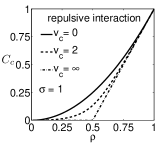
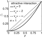
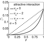
Figure 2: Contact correlators $C_{c}=C_{i-\sigma,i}$ for spatially homogeneous systems of hard rods of sizes $\sigma=1$ and 5, and different strength of repulsive and attractive contact interactions $v_{c}=v_{i-\sigma,i}$.

III Density functionals

Based on the Gibbs-Bogoliubov inequality the following functional is defined in density functional theory,

$$\Omega[\mathbf{p}] =\sum_{\mathbf{n}}\chi_{\mathbf{p}}(\mathbf{n})\left[\ln\chi_{\mathbf{p}}(\mathbf{n})+V(\mathbf{n})+U(\mathbf{n})-\mu N\right]$$

$$=F[\mathbf{p}]+\sum_{k=1}^{L}(u_{k}-\mu)p_{k}\,,$$ (14)

where $F[\mathbf{p}]=\sum_{\mathbf{n}}\chi_{\mathbf{p}}(\mathbf{n})[\ln\chi_{\mathbf{p}}(\mathbf{n})+V(\mathbf{n})]$ is the free energy functional and the $u_{k}$ is the external in Eq. (1). Minimizing $\Omega[\mathbf{p}]$ yields the equilibrium density profile $\mathbf{p}^{eq}=\{p_{i}^{eq}\}$.

Substituting the results of Sec. II and using the abbreviated notation, $\Phi(x):=x\ln x$, we can write the free-energy functional in the form

$$F[\mathbf{p}] =\sum_{i,j}v_{i,j}C_{i,j}$$

$${}+\sum_{s=1}^{L}\Biggl{\{}\Phi\Bigl{(}p_{s}\!-\!\sum_{i=s-\xi}^{s-\sigma}C_{s,i}\Bigr{)}$$

$$\phantom{{}+\sum_{s=1}^{L}\Bigl{\{}}{}+\Phi\Bigl{(}1\!-\!\sum_{i=s-\xi}^{s}p_{i}\!+\!\sum_{i=s-\xi+\sigma}^{s}\sum_{j=s-\xi}^{i-\sigma}C_{i,j}\Bigr{)}$$

$$\phantom{{}+\sum_{s=1}^{L}\Bigl{\{}}{}-\Phi\Bigl{(}1\!-\!\sum_{i=s-\xi}^{s-1}p_{i}+\sum_{i=s-\xi+\sigma}^{s-1}\sum_{j=s-\xi}^{i-\sigma-1}C_{i,j}\Bigr{)}$$

$$\phantom{{}+\sum_{s=1}^{L}\Bigl{\{}}{}+\sum_{i=s-\xi}^{s-\sigma}\Bigl{\{}\Phi\Bigl{(}C_{s,i}\Bigr{)}+\Phi\Bigl{(}p_{i}-\sum_{j=i+\sigma}^{s}C_{j,i}\Bigr{)}$$

$$\phantom{{}+\sum_{s=1}^{L}\Bigl{\{}{}+\sum_{i=s-\xi}^{s-\sigma}\Bigl{\{}}{}-\Phi\Bigl{(}p_{i}-\sum_{j=i+\sigma}^{s-1}C_{j,i}\Bigr{)}\Bigr{\}}\Biggr{\}}\,,$$ (15)

with the $C_{i,j}=C_{i,j}[\mathbf{p}]$ extracted from Eq. (10). For contact interactions, $v_{c}\equiv v_{i,i+\sigma}$, it can be rendered more compactly:

$$F[\mathbf{p}] =\sum\limits_{s}\Bigl{\{}C_{s-\sigma,s}v_{s-\sigma,s}+\Phi\Bigl{(}p_{s}-C_{s-\sigma,s}\Bigr{)}$$ (16)

$${}+\Phi\Bigl{(}1-\sum_{k=s-\sigma}^{s}p_{k}+C_{s-\sigma,s}\Bigr{)}-\Phi\Bigl{(}1-\sum_{k=s-\sigma}^{s-1}p_{k}\Bigr{)}$$

$${}+\Phi\Bigl{(}C_{s-\sigma,s}\Bigr{)}+\Phi\Bigl{(}p_{s-\sigma}-C_{s-\sigma,s}\Bigr{)}-\Phi\Bigl{(}p_{s-\sigma}\Bigr{)}\Bigl{\}}$$

For the special case $\sigma=1$ (Ising lattice gas), this functional agrees with a previous result of Ref. Buschle et al., 2000a, for which Lafuente and Cuesta Lafuente and Cuesta (2005) derived a fundamental measure form also. As it happens, the fundamental measure form can be extended to hard rods ($\sigma>1$) with contact interaction by eliminating $v_{i,i+\sigma}C_{i,i+\sigma}$ in Eq. (16) in favor of correlators and densities via Eq. (10):

$$F[\mathbf{p}] =\sum_{s=1}^{L}\left(\mathcal{F}_{2}[p_{s-\sigma},\ldots,p_{s}]-\mathcal{F}_{1}[p_{s-\sigma},\ldots,p_{s-1}]\right)$$ (17)

where

$$\mathcal{F}_{1}[p_{s-\sigma},\ldots,p_{s-1}]=$$

$$\hskip 20.00003ptp_{s-\sigma}\ln p_{s-\sigma}+(1-\sum_{i=s-\sigma}^{s-1}p_{i})\ln(1-\sum_{i=s-\sigma}^{s-1}p_{i})$$ (18)

and

$$\mathcal{F}_{2}[p_{s-\sigma},\ldots,p_{s}]=$$

$$\hskip 30.00005ptp_{s}\ln(p_{s}-C_{s-\sigma,s})+p_{s-\sigma}\ln(p_{s-\sigma}-C_{s-\sigma,s})$$

$$\hskip 30.00005pt{}+(1-\sum_{i=s-\sigma}^{s}p_{i})\ln(1-\sum_{i=s-\sigma}^{s}p_{i}+C_{s-\sigma,s})$$ (19)

are the free energy functionals of one-particle and two-particle cavities, respectively. A one-particle cavity refers to a range of successive lattice sites, where at most one occupation number can be one, in analogy to the zero-dimensional cavity in Rosenfeld’s fundamental measure theory in continuous space. For discrete lattice gas systems, following Lafuente and Cuesta, Lafuente and Cuesta (2005) an $m$-particle cavity refers to a range of successive lattice sites, where at most $m$ occupation numbers can be one. Notice that the size of an $m$-particle cavity can vary between $m\sigma$ (minimal $m$-particle cavity) and $(m+1)\sigma-1$ (maximal $m$-particle cavity). In this respect, $\mathcal{F}_{1}$ in Eq. (III) refers to a maximal one-particle cavity and $\mathcal{F}_{2}$ in Eq. (III) to a minimal two-particle cavity. Fundamental measure forms allow for a straighforward extension to approximate functionals in higher dimensions that become exact under dimensional reduction.Rosenfeld (1989); Lafuente and Cuesta (2005)

IV Thermodynamics of homogeneous systems

Here the focus is entirely on bulk thermodynamic properties of homogeneous systems with attractive or repulsive contact interactions. The internal energy per site $u_{\scriptscriptstyle\rm int}=U_{\scriptscriptstyle\rm int}/L$ is directly related to the contact correlator $C_{c}$ from Eq. (12):

$$u_{\scriptscriptstyle\rm int}(p)=v_{c}C_{c}(p).$$ (20)

Its dependence on coverage $\rho$ for $\sigma=1,5$ is represented by the curves in Fig. 2, appropriately rescaled by $v_{c}$ (positive or negative). Not surprisingly, the magnitude of $u_{\scriptscriptstyle\rm int}$ increases with crowding. We infer the free energy per site $f=F/L$ from Eq. (16):

$$f(p) =(1-(\sigma+1)p)\ln(1-(\sigma+1)p+C)$$

$$+2p\ln(p-C)-(1-\sigma p)\ln(1-\sigma p)-p\ln p.$$ (21)

The entropy per site $s=S/L$ follows directly:

$$s(p)=u(p)-f(p).$$ (22)

Their dependences on $\rho$ are shown in Figs. 3 and 4.

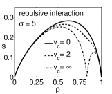
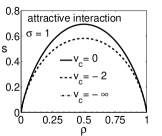
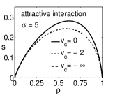
Figure 3: Entropy $s$ per lattice site as a function of the coverage $\rho$ for a homogeneous system of hard rods of sizes $\sigma=1$ and 5, and various contact interactions $v_{c}$.

Attractive and repulsive contact interactions both lead to an entropy reduction. The underlying causes are different. For $v_{c}<0$ the rods have a tendency to form clusters. This ordering tendency is largely independent of coverage, producing a relative entropy reduction that depends only weakly on $\rho$. In the limit $v_{c}\to-\infty$, the rods form a single cluster, implying $s=0$ for any $\rho$.

For $v_{c}>0$, by contrast, the rods have a tendency to disperse, i.e. to avoid contact. The associated ordering tendency in the face of space constraints strongly depends on coverage. Above a critical strength $v_{c}^{\star}\cong 1.95$ of the contact interaction, the entropy develops a double-hump structure with a minimum at $\rho=1/2$ for $\sigma=1$, and close to $\sigma/(\sigma+1)$ for $\sigma>1$. At the coverage $\rho=\sigma/(\sigma+1)$, perfect ordering, corresponding to a vanishing entropy, is obtained in the limit $v_{c}\to+\infty$ ($v_{c}\gg v_{c}^{\star}$). For lower or higher coverages, residual entropy $s$ persists at significant levels. Entropy profiles similar to those in Fig. 3 were recently found by a study of jammed granular matter in a narrow channel.Gundlach et al. (2013)

A point of some interest is the location of the entropy maximum in dependence of $\sigma$ and $v_{c}$ (first maximum for $v_{c}>v_{c}^{\star}$ in the case of repulsive interactions). The curves show that for $v_{c}=0$ the coverage of maximum entropy shifts to right from $\rho=1/2$ as the size of the rods grows from $\sigma=1$ and that, for given $\sigma>1$, it shift to left as $|v_{c}|$ increases. This shift can be understood intuitively by viewing rods and vacancies as two species with numbers $N_{\rm rod}=pL=\rho L/\sigma$ and $N_{\rm vac}=(1-\rho)L$, respectively. Neglecting entropy related correlation effects in the non-interacting case, the number $\sim e^{sL}$ of possible configurations could then be estimated by $(N_{\rm rod}+N_{\rm vac})!/(N_{\rm rod}!N_{\rm vac}!)$. For $\sigma=1$, this is clearly maximal for equal number of particles and vacancies $(\rho=1/2)$, while for $\sigma>1$, one has to take into account that $(N_{\rm rod}+N_{\rm vac})$ decreases with increasing $\rho$. Accordingly, the location of the entropy maximum occurs left to $\rho=\sigma/(\sigma+1)$, where $N_{\rm rod}=N_{\rm vac}$. In the interacting case, the coverage of maximum entropy moves to the left for increasing interaction strength, because the enhanced configurational restrictions for larger $|v_{c}|$ can be partly compensated by lowering $\rho$. Analytical results for the entropy of hard rods with nearest-neighbor interactions in one-dimensional continuum have been earlier obtained by Percus.Percus (1989) Its overall behavior as function of the density in the case of contact interaction agrees with the one displayed in Fig. 3.

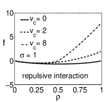
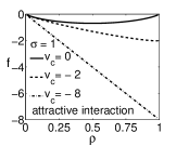
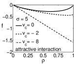
Figure 4: Free energy per site versus $\rho$ for a homogeneous system of hard rods of sizes $\sigma=1$ and 5, and various contact interactions $v_{c}$.

Because of absence of phase transitions in one dimension (if not considering “exotic” cases of interaction with particular long-range behavior Berlin and Kac. (1952)) the free energy shown in Fig. 4 does not show any peculiarities as a function of $\rho$. In the case of attractive interaction, it approaches the line $f\sim-|v_{c}|\rho/\sigma$ for large $|v_{c}|$ due to the aggregation of the rods into one cluster. For strong repulsive interactions, i.e. for $v_{c}$ significantly larger than $v_{c}^{\star}$, the free energy essentially follows the (negative) entropy for $\rho\lesssim\sigma/(\sigma+1)$, increases linearly for $\rho\gtrsim\sigma/(\sigma+1)$ due to the linear increase of non-avoidable contacts until reaching $C_{c}v_{c}\simeq v_{c}/\sigma$ for $\rho\to 1$.

For repulsive interactions, the density $\rho=\sigma/(\sigma+1)$ should also show up as a particular value in the behavior of the chemical potential, because the free energy amount to add a rod to the system is expected to increase strongly around this point. The chemical potential $\mu=\partial f/\partial\rho$ is given by

$$\mu=\ln\left\{\frac{\sigma C}{\rho e^{-v}e^{1-\sigma}}\right\}+\sigma\ln\left\{\left[\frac{1-\rho}{1-(\sigma+1)\rho/\sigma+C}\right]\right\}$$ (23)

and plotted in Fig. 5 as function of $\rho$. It indeed shows a step-like change around $\rho=\sigma/(\sigma+1)$ for strong repulsive interactions, which could be utilized for determining the rod size from thermodynamic measurements. For comparison the behavior for attractive interaction is also displayed in Fig. 5.

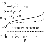
Figure 5: Chemical potential $\mu$ as a function of the coverage $\rho$ for a homogeneous system of hard rods of sizes $\sigma=1$ and 5, and various contact interactions $v_{c}$.

V Conclusions

Our solution for the distribution of microstates of hard-rod lattice gases with a general nearest-neighbor-range interaction potential provides a promising basis for future studies related to applications. For example, the results can be utilized to describe formation of molecular nanowires on surfaces, where molecules interact via van der Waals interactions and form hydrogen bonds when coming into contact. In the model, such situation could be accounted for by an interaction profile $v_{i,j}$ with strong attractive interaction $v_{i,i+\sigma}<0$ at contact distance $\sigma$ and a smoothly decreasing, weaker attractive part for $\sigma<|i-j|<2\sigma$. Also, based on experiences in other contexts, Dierl et al. (2011, 2012) the explicit exact expressions for the density functionals should allow one to faithfully study the kinetics of wire formation by employing time-dependent density functional theory. Similarly, our results may be helpful in the future to treat diffusion of molecules through nanopores or membrane channels.

Our derivation of a fundamental measure form of the hard-rod lattice gas with contact interaction enables a straightforward extension to higher dimensions. This should be useful to account for transitions between different phases in corresponding systems, which generally resemble nematic (and other) phases of liquid crystals.Martínez-Ratón (2007); Martínez-Ratón et al. (2008); de las Heras et al. (2010) It has been shown Lafuente and Cuesta (2002, 2003a) for athermal hard-rod lattice gases ($v_{i,j}=0$) that extensions to higher dimensions are a powerful means to treat corresponding phase transitions. Up to now, we did not succeed to identify fundamental measure forms for general nearest-neighbor-range interactions $v_{i,j}$. However, there seem to be other possibilities of extensions, which become exact under dimensional reduction. These will be explored elsewhere.

Considering the core in the derivation of the distribution of microstates, it is important to realize that the procedure can in principle be extended to interactions of longer range covering several rod lengths. For a given range $\xi$, the exclusion constraint leads to a natural decomposition of the set $\{\mathbf{n}\}_{s}=\{n_{s},\ldots,n_{s-\xi}\}$ into ranges covering the lattice sites $s-\sigma+1,\ldots,s$ (first range), $s-2\sigma+1,\ldots,s-\sigma$ (second range), and so on. In each of these ranges at most one occupation number can be equal to one. The total number of ranges that need to be taken into account is $\lceil\xi/\sigma\rceil$, where $\lceil x\rceil$ denotes the integer ceiling division, i.e. the smallest integer larger than $x$. Accordingly, we would need to consider higher-order correlators $C(1_{i_{1}},1_{i_{2}},1_{i_{3}},\ldots,...)$, where $1_{i_{k}}$, specifies the location of the occupied site in the $k$th range as in Sec. II.2. The distribution of microstates can then be expressed in term of these correlators $C(1_{i_{1}},1_{i_{2}},1_{i_{3}},\ldots,...)$ and the densities $p_{i}$. By equating with the Boltzmann formula for simple configurations, relations between the $C(1_{i_{1}},1_{i_{2}},1_{i_{3}},\ldots,...)$ and the $p_{i}$ eventually can be obtained, which need to be solved for expressing the $C(1_{i_{1}},1_{i_{2}},1_{i_{3}},\ldots,...)$ in terms of the $p_{i}$.

By working out the long-range asymptotic behavior of correlation functions it should be possible also to study the occurrence and behavior of Widom-Fisher lines.Fisher and Widom (1969) These lines separate regions in the temperature-density and temperature-pressure planes, where in one region the pair correlation decays monotonically, while in the other region it oscillates with decaying amplitude. The abrupt change in the behavior at the lines takes place without any singularities in the thermodynamics. In the original work, Fisher and Widom (1969) transition lines were calculated for a one-dimensional continuum fluid with square-well interaction potential and a lattice fluid as considered in this work, corresponding to hard rods of size $\sigma=2$ with first-neighbor coupling. Access to the correlation properties of systems with larger $\sigma$ and interactions of longer range may allow one to gain deeper insight into general features of these lines.

Let us finally note that the rod length defines a length scale independent of the lattice spacing, which implies that a continuum limit of the results should be accessible. This, the possible extension to larger interaction ranges, and evaluations of Widom-Fisher lines open new and challenging possibilities for further investigations.