Quantum Effects near Charged Dilatonic Black Holes

Abstract

The expectation value $\langle\varphi^{2}\rangle$ in the Hartle-Hawking vacuum is calculated for minimally-coupled neutral scalar fields at the horizon of a charged dilatonic black hole.

Some exotic classes of black holes have attracted much attention of modern theoretical physicists. For example, black holes with quantum hair are discovered recently.[1, 2, 3, 4, 5] The thermodynamical properties of the black holes are expected to receive some corrections at the presence of quantum hair. As another example, we mention the study on the properties of dilatonic black holes in two-dimensional space-time.[6] The black holes in two dimensions are known to be concerned with conformal field theory.[6] Furthermore, they are useful tools for the nonperturbative study on the evaporation of black holes.[7, 8]

A charged, dilatonic black hole in four (or more) dimensions is now a very popular object [9, 10]; various aspects of their classical and quantum properties are curious and worth studying.[11, 12, 13, 14, 15, 16, 17, 18, 19] In this paper, we treat this charged dilatonic black hole in four dimensions. The first motivation to introduce the dilatonic black holes originates from string theory. The interpolation between the stringy (dilatonic) electromagnetism and the usual Maxwell system has been considered by introducing an arbitrary value for dilaton coupling “$a$” to the Maxwell field. The action which governs the system can be written as

$$S=\int d^{4}x\frac{\sqrt{-g}}{16\pi}[R-2(\nabla\phi)^{2}-e^{-2a\phi}F^{2}]\,,$$ (1)

where $R$ is the scalar curvature, $\phi$ is the dilaton and $F$ is the field strength of the Maxwell field. The special choice $a=1$ does correspond to the string effective action. The study on the system with arbitrary values for dilaton coupling shows clearly the effect of adding the dilaton.

In this paper, we study the vacuum polarization in a background of the charged dilatonic black holes. This is expected to be closely connected to the thermal description of the black holes. We compute the quantity $\langle\varphi^{2}\rangle$ for minimally-coupled real scalar fields at the horizon, as the simplest example.

The metric for a spherically symmetric charged dilatonic black hole in the Einstein-Maxwell-dilaton system with an arbitrary dilaton coupling, $a$, is written in the form [9, 10]

$$ds^{2}=-\Delta\sigma^{-2}dt^{2}+\sigma^{2}(\Delta^{-1}dr^{2}+r^{2}d\Omega^{2}_{2})\,,$$ (2)

where

$$\Delta(r)=\left(1-\frac{r_{+}}{r}\right)\left(1-\frac{r_{-}}{r}\right)\quad\mbox{and}\quad\sigma^{2}(r)=\left(1-\frac{r_{-}}{r}\right)^{2a^{2}/(1+a^{2})}\,.$$ (3)

Here $d\Omega^{2}_{2}$ is the standard line element for a sphere with unit radius.

In these expressions $r_{+}$ and $r_{-}$ are integration constants and they are connected to the mass $M$ and electric charge $Q$ of the black hole through the relations

$$2M=r_{+}+\frac{1-a^{2}}{1+a^{2}}r_{-}\quad\mbox{and}\quad Q^{2}=\frac{r_{+}r_{-}}{1+a^{2}}\,,$$ (4)

the horizon length is $r_{+}$.

The configurations of the dilaton $\phi$ and electric fields are given by

$$e^{2a\phi}=\sigma^{2}(r)\quad\mbox{and}\quad F=\frac{Q}{r^{2}}dt\wedge dr\,,$$ (5)

respectively.

One can easily see that the geometry of the fields reduces to the Reissner- Nordström space-time when $a=0$. The case with $a=1$ corresponds to string theory.

Now let $\varphi$ be a real scalar field which couples minimally to the scalar curvature of the space-time. Here we treat the Hartle-Hawking vacuum.[20] We take the vacuum polarization $\langle\varphi^{2}\rangle$ as the coincident limit of the two-point function $\langle\varphi(x)\varphi(x^{\prime})\rangle$ with proper regularization.[21, 22, 23, 24, 25, 26, 27, 28, 29, 30] Then the two-point function of the scalar field can be obtained most clearly by the mode-sum method. We have to find the solution for the wave equation in a background geometry of the charged dilatonic black hole (2) with Euclidean signature.

If it is required that there is no singularity at the horizon $r=r_{+}$ in the Euclideanized geometry, the Euclidean time $\tau$ must be periodic with period $1/T_{H}$, where $T_{H}$ is the Hawking temperature [9, 10, 11, 12]

$$T_{H}=\frac{1}{4\pi r_{+}}\left(1-\frac{r_{-}}{r_{+}}\right)^{(1-a^{2})/(1+a^{2})}\,.$$ (6)

A mode function for the solution of the massless Klein-Gordon equation can be written as

$$\varphi_{nlm}=R_{nl}(r)Y_{lm}(\theta,\varphi)e^{-i2\pi nT_{H}\tau}\,,$$ (7)

where $Y_{lm}(\theta,\varphi)$ is the spherical harmonics.

To make the differential equation for the radial function a simpler form, we use a new variable $y$ defined by the relation

$$y=r-r_{-}\,.$$ (8)

Then the radial function is the solution of the following differential equation:

$$\frac{d}{dy}\left\{y^{2}\left(1-\frac{y_{H}}{y}\right)\frac{dR(y)}{dy}\right\}$$

$$\qquad-(2\pi nT_{H})^{2}y^{2}\frac{\left(1+\frac{r_{-}}{y}\right)^{2/(1+a^{2})}}{1-\frac{y_{H}}{y}}R(y)-l(l+1)R(y)=0\,,$$ (9)

where $y_{H}=r_{+}-r_{-}$.

One can immediately realize that the solution for (9) will have non-analytic expression in general. Only $n=0$ mode is exactly soluble in the form of the special function.

The $n=0$ mode takes exactly the same form as in the case with the Schwarzchild space time treated in Ref. [26] by Frolov et al. Of course, the higher modes are quite different. But, if we need only the two-point Hamilton one of which point lies on the horizon membrane ($r=r_{+}$), the contribution from the higher modes becomes irrelevant for the situation.

Thus the procedure from now on must be similar to the method adopted by Frolov et al.[26] The quantity $\langle\varphi(x)\varphi(x^{\prime})\rangle$ behaves like that in Frolov’s case as long as the point $x$ lies on the horizon membrane. The only difference is the overall coefficient proportional to the Hawking temperature $T_{H}$. Therefore, it depends on the value of dilaton coupling only through the coefficient. When the separation is restricted to the radial direction, the two-point function takes the form,

$$\langle\varphi(x)\varphi(x^{\prime})\rangle=\frac{\left(1-\frac{r_{-}}{r_{+}}\right)^{-2a^{2}/(1+a^{2})}}{16\pi^{2}r_{+}^{2}\sinh^{2}\eta}$$ (10)

where $x=(\tau,y_{H},\theta,\varphi)$ and $x^{\prime}=(\tau,y,\theta,\varphi)$. $\eta$ is defined by

$$\cosh\eta=\left(\frac{y}{y_{H}}\right)^{1/2}\,.$$ (11)

To compute the vacuum polarization $\langle\varphi^{2}\rangle(x)$, where $x$ is located on the horizon, we must subtract the divergence part of the two-point function. The higher order in the Schwinger-de Witt expansion of the propagator (two-point function) with respect to the powers of the geodesic distance between the two points are not yet known; moreover, as the present case, the coefficients for the expansion takes awkward forms for non-conformally-coupled fields. Fortunately, the scalar curvature vanishes at the horizon $r=r_{+}$ ($y=y_{H};\eta=0$) of the charged dilatonic black hole in four dimensions. (This does not hold in other dimensions.)

Taking such things into consideration, the divergent and constant contributions in the Schwinger-de Witt expansion near the horizon is written by the use of the geodesic distance and the Ricci curvature as [25]

$$\langle\varphi(x)\varphi(x^{\prime})\rangle_{div}=\frac{\Delta^{1/2}}{8\pi^{2}\sigma(x,x^{\prime})}=\frac{1}{8\pi^{2}\sigma(x,x^{\prime})}\left(1+\frac{1}{12}R_{\alpha\beta}\sigma^{,\alpha}\sigma^{,\beta}\right)\,,$$ (12)

where $\sigma=s^{2}/2$ and $s(x,x^{\prime})$ is the geodesic distance between $x$ and $x^{\prime}$. For radial separation, $s$ is given by

$$s=\int_{y_{H}}^{y}\frac{\left(1+\frac{r_{+}}{y}\right)^{1/(1+a^{2})}}{\sqrt{1-\frac{y_{H}}{y}}}$$

$$=2y_{H}\left(1-\frac{r_{-}}{r_{+}}\right)^{-1/(1+a^{2})}\int_{0}^{\eta}\cosh^{2}\eta\left(1-\frac{r_{-}}{r_{+}}\tanh^{2}\eta\right)^{1/(1+a^{2})}d\eta$$

$$=2r_{+}\left(1-\frac{r_{-}}{r_{+}}\right)^{-a^{2}/(1+a^{2})}\left(\eta+\frac{1}{3}\left(1-\frac{r_{-}}{(1+a^{2})r_{+}}\right)\eta^{3}+O(\eta^{5})\right)\,,$$ (13)

and

$$R_{\alpha\beta}\frac{\sigma^{,\alpha}\sigma^{,\beta}}{\sigma}=2R^{y}_{y}=-\frac{2Q^{2}}{r_{+}^{4}}\left(1-\frac{r_{-}}{r_{+}}\right)^{-2a^{2}/(1+a^{2})}\,.$$ (14)

Using these and (4), we get the final result:

$$\langle\varphi^{2}\rangle_{horizon} = \lim_{x^{\prime}\rightarrow x}(\langle\varphi(x)\varphi(x^{\prime})\rangle-\langle\varphi(x)\varphi(x^{\prime})\rangle_{div})$$ (15)

$$= \frac{1}{48\pi^{2}r_{+}^{2}}\left(1-\frac{r_{-}}{(1+a^{2})r_{+}}\right)\left(1-\frac{r_{-}}{r_{+}}\right)^{-2a^{2}/(1+a^{2})}\,.$$

We display the result in Figs. 1 and 2 in two different manners. Figures $1a,b$ show $16\pi^{2}M^{2}\langle\varphi^{2}\rangle$ at the horizon versus $q^{2}=Q^{2}/\{(1+a^{2})M^{2}\}$ for $a^{2}=0,1/3,1,3$, while Fig. 2 shows $\langle\varphi^{2}\rangle/(4T_{H}^{2})$ at the horizon versus $q^{2}$ for $a^{2}=0,1/3,1,3$.

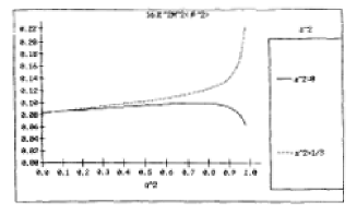
(a)

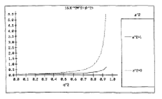
(b)

Figure 1: (a) $16\pi^{2}M^{2}\langle\varphi^{2}\rangle$ at the horizon is plotted against $q^{2}=Q^{2}/\{(1+a^{2})M^{2}\}$ for $a^{2}=0,1/3$; (b) $16\pi^{2}M^{2}\langle\varphi^{2}\rangle$ at the horizon is plottad against $q^{2}$ for $a^{2}=1,3$.

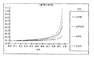
Figure 2: $\langle\varphi^{2}\rangle/(4T_{H}^{2})$ at the horizon is plotted against $q^{2}$ for $a^{2}=0,1/3,1,3$.

In the extremal limit, $q\rightarrow 1$, $\langle\varphi^{2}\rangle$ diverges in general, except for $a=0$ case, i.e., the Reissner-Nordström space-time. The ratio $\langle\varphi^{2}\rangle/(4T_{H}^{2})$ diverges regardless of the value for $a$.

We have found that the critical value for $a$ is zero when we pay attention to the vacuum polarization at the horizon of the maximally charged dilatonic black hole.

In this paper, we discussed only minimally coupled scalar field. The couplings to the dilaton field as well as the curvature will change the behavior of the quantum fields; besides, the connection to the thermodynamics of black holes and the quantum effects in the other vacua are to be studied. The relationship to supersymmetry is also of great interest.

References

- [1] J. Preskill, Phys. Scripta T36 (1991) 258.
- [2] S. Coleman, J. Preskill and F. Wilczek, Mod. Phys. Lett. A6 (1991) 1631.
- [3] S. Coleman, J. Preskill and F. Wilczek, Phys. Rev. Lett. 67 (1991) 1975.
- [4] S. Coleman, J. Preskill and F. Wilczek, Nucl. Phys. B378 (1992) 175.
- [5] K. Shiraishi, Europhys. Lett. 20 (1992) 483.
- [6] E. Witten, Phys. Rev. D44 (1991) 314.
- [7] C. G. Callan, S. B. Giddings, J. A. Harvey and A. Strominger, Phys. Rev. D45 (1992) R1005.
- [8] T. Banks, A. Dabholker, M. R. Douglas and M. O’Loughlin, Phys. Rev. D45 (1992) 3607.
- [9] G. W. Gibbons and K. Maeda, Nucl. Phys. B298 (1988) 741.
- [10] D. Garfinkle, G. Horowitz and A. Strominger, Phys. Rev. D43 (1991) 3140; D45 (1992) 3888(E).
- [11] J. Preskill, P. Schwarz, A. Shapere, S. Trivedi and F. Wilczek, Mod. Phys. Lett. A6 (1991) 2353.
- [12] C. F. E. Holzhey and F. Wilczek, Nucl. Phys. B388 (1992) 447.
- [13] K. Shiraishi, Phys. Lett. A166 (1992) 298.
- [14] H. Horne and G. T. Horowitz, Phys. Rev. D46 (1992) 1340.
- [15] A. Sen, Phys. Rev. Lett. 69 (1992) 1006.
- [16] K. Shiraishi, J. Math. Phys. 34 (1992) 1480.
- [17] K. Shiraishi, Nucl. Phys. B402 (1993) 399.
- [18] K. Shiraishi, Int. J. Mod. Phys. D2 (1993) 59.
- [19] K. Shiraishi, Mod. Phys. Lett. A7 (1992) 3449.
- [20] J. B. Hartle and S. W. Hawking, Phys. Rev. D13 (1976) 2188.
- [21] P. Candelas, Phys. Rev. D21 (1980) 2185.
- [22] P. Candelas and K. W. Howard, Phys. Rev. D29 (1984) 1618.
- [23] K. W. Howard and P. Candelas, Phys. Rev. Lett. 53 (1984) 403.
- [24] K. W. Howard, Phys. Rev. D30 (1984) 2532.
- [25] V. P. Frolov, Phys. Rev. D26 (1982) 954.
- [26] V. P. Frolov, F. D. Mazzitelli and J. P. Paz, Phys. Rev. D40 (1989) 948.
- [27] I. D. Novikov and V. P. Frolov, Physics of Black Holes (Kluwer Academic Publishers, 1988).
- [28] V. P. Frolov, in Trends in Theoretical Physics, ed. P. J. Ellis and Y. C. Tang (Addison Wesley, 1991), pp. 27–75.
- [29] P. R. Anderson, Phys. Rev. D39 (1989) 3785.
- [30] P. R. Anderson, Phys. Rev. D41 (1990) 1152.