Nonparametric Identification in Panels using Quantiles

Abstract

This paper considers identification and estimation of ceteris paribus effects of continuous regressors in nonseparable panel models with time homogeneity. The effects of interest are derivatives of the average and quantile structural functions of the model. We find that these derivatives are identified with two time periods for “stayers”, i.e. for individuals with the same regressor values in two time periods. We show that the identification results carry over to models that allow location and scale time effects. We propose nonparametric series methods and a weighted bootstrap scheme to estimate and make inference on the identified effects. The bootstrap proposed allows uniform inference for function-valued parameters such as quantile effects uniformly over a region of quantile indices and/or regressor values. An empirical application to Engel curve estimation with panel data illustrates the results.

Keywords: Panel data, nonseparable model, average effect, quantile effect, Engel curve

1 Identification for Panel Regression

A frequent object of interest is the ceteris paribus effect of $x$ on $y,$ when observed $x$ is an individual choice variable partly determined by preferences or technology. Panel data holds out the hope of controlling for individual preferences or technology by using multiple observations for a single economic agent. This hope is particularly difficult to realize with discrete or other nonseparable models and/or multidimensional individual effects. These models are, by nature, not additively separable in unobserved individual effects, making them challenging to identify and estimate.

A fundamental idea for using panel data to identify the ceteris paribus effect of $x$ on $y$ is to use changes in $x$ over time. In order for changes over time in $x$ to correspond to ceteris paribus effects, the distribution of variables other than $x$ must not vary over time. This restriction is like “time being randomly assigned” or ”time is an instrument.” In this paper we consider identification via such time homogeneity conditions. They are also the basis of many previous panel results, including Chamberlain (1982), Manski (1987), and Honore (1992). Recently time homogeneity has been used as the basis for identification and estimation of nonseparable models by Chernozhukov, Fernandez-Val, Hahn, Newey (2013), Evdokimov (2010), Graham and Powell (2012), and Hoderlein and White (2012). Because economic data often exhibits drift over time, we also allow for some time effects, while maintaining underlying time homogeneity conditions.

In this paper we give identification and estimation results for quantile effects with time homogeneity and continuous regressors. The effects of interest are derivatives of quantile structural functions of the model. We find that these derivatives are identified with two time periods for “stayers”, i.e. conditional on $x$ being equal in two time periods. Time homogeneity is too strong for many econometric applications where time trends are evident in the data. We weaken homogeneity by allowing for location and scale time effects. Allowing for such time effects makes identification and estimation more complicated but more widely applicable. We also give analogous results for conditional mean effects under weaker identification conditions than previously.

Quantile identification under time homogeneity is based on differences of quantiles. It is also interesting to consider whether quantiles of differences can help identify effects of interest. We do not find that time homogeneity alone can lead to identification from quantiles of differences. We do give quantile difference identification results that restrict the distribution of individual effects conditional on $x$, similarly to Chamberlain (1980), Altonji and Matzkin (2005), and Bester and Hansen (2009). In our opinion these added restrictions make quantiles of differences less appealing. We therefore focus for the rest of the paper, including the application, on differences of quantiles.

To illustrate we provide an application to Engel curve estimation. The Engel curve describes how demand changes with expenditure. We use data from the 2007 and 2009 waves of the Panel Study of Income Dynamics (PSID). Endogeneity in the estimation of Engel curves arises because the decision to consume a commodity may occur simultaneously with the allocation of income between consumption and savings. In contrast with the previous cross sectional literature, we do not rely on a two-stage budgeting argument that justifies the use of labor income as an instrument for expenditure. Instead, we assume that the Engel curve relationships are time homogeneous up to location and scale time effects, which leads to identification of structural effects from panel data.

An alternative approach to identification in panel data is to impose restrictions on the conditional distribution of the individual effect given $x$. This approach leads to nonparametric generalizations of Chamberlain’s (1980) correlated random effects model. As shown by Chamberlain (1984), Altonji and Matzkin (2005), Bester and Hansen (2009), and others, this kind of condition leads to identification of various effects. In particular, Altonji and Matzkin (2005) show identification of an average derivative conditional on the regressor equal to a specific value, an effect they call the local average response (LAR). In this paper we take a different approach, preferring to impose time homogeneity rather than restrict the relationship between observed regressors and unobserved individual effects. We refer to Hsiao (2003) for a broader perspective of panel data models.

Section 2 describes the model and gives an average derivative result. Section 3 gives the quantile identification result that follows from time homogeneity. Section 4 considers how quantiles of differences can be used to identify the effect of $x$ on $y$. Section 5 explains how we allow for time effects. Estimation and inference are briefly discussed in Section 6, and the empirical example is given in Section 7. The Appendix contains the proofs of the main results.

2 The Model and Conditional Mean Effects

The data consist of $n$ observations on ${\boldsymbol{Y}}_{i}=(Y_{i1},\ldots,Y_{iT})^{\prime}$ and ${\boldsymbol{X}}_{i}=[X_{i1}^{\prime},\ldots,X_{iT}^{\prime}]^{\prime}$, for a dependent variable $Y_{it}$ and a vector of regressors $X_{it}$. Throughout we assume that the observations $({\boldsymbol{Y}}_{i},{\boldsymbol{X}}_{i})$, $(i=1,\ldots,n)$, are independent and identically distributed. The nonparametric models we consider satisfy

Assumption 1.

There is a function $\phi$ and vectors of random variables $A_{i}$ and $V_{it}$ such that

$$Y_{it}=\phi(X_{it},A_{i},V_{it}),\qquad i=1,\ldots,n,\quad t=1,2,\ldots,T.$$

We focus in this paper on the two time period case, $T=2$, though it is straightforward to extend the results to many time periods. The vector $A_{i}$ consists of time invariant individual effects that often represent individual heterogeneity. The vector $V_{it}$ represents period specific disturbances. Altonji and Matzkin (2005) considered models satisfying Assumption 1. As discussed in Chernozhukov et. al. (2013), the invariance of $\phi$ over time in this Assumption does not actually impose any time homogeneity. If there are no restrictions on $V_{it}$ then $t$ could be one of the components of $V_{it},$ allowing the function to vary over time in a completely general way. The next condition together with Assumption 1 imposes time homogeneity on the model.

Assumption 2.

$V_{it}|{\boldsymbol{X}}_{i},A_{i}\overset{d}{=}V_{i1}|{\boldsymbol{X}}_{i},A_{i}$  for all $t.$

This is a static, or ”strictly exogenous” time homogeneity condition, where all leads and lags of the regressor are included in the conditioning variable ${\boldsymbol{X}}_{i}.$ It requires that the conditional distribution of $V_{it}$ given ${\boldsymbol{X}}_{i}$ and $A_{i}$ does not depend on $t,$ but does allow for dependence of $V_{it}$ over time. This assumption rules out dynamic models where lagged values of $Y_{it}$ are included in $X_{it}.$

Setting $U_{it}=(A_{i}^{\prime},V_{it}^{\prime})^{\prime}$, an equivalent condition is

$$U_{it}|{\boldsymbol{X}}_{i}\overset{d}{=}U_{i1}|{\boldsymbol{X}}_{i}.$$

Thus, the time invariant $A_{i}$ has no distinct role in this model. As further discussed in Chernozhukov et. al. (2013), this seems a basic condition that helps panel data provide information about the effect of $x$ on $y.$ It is like the time period being ”randomly assigned” or ”time is an instrument,” with the distribution of factors other than $x$ not varying over time, so that changes in $x$ over time can help identify the effect of $x$ on $y$.

Although they seem useful for nonlinear models, the time homogeneity conditions are strong. In particular they do not allow for heteroskedasticity over time, which is often thought to be important in applications. We partially address this problem below by allowing for location and scale time effects.

For notational convenience we shall drop the $i$ subscript and let $T=2$ in the following. Our focus in this paper is on the case where the regressors ${\boldsymbol{X}}$ are continuously distributed. We will be interested in several effects of ${\boldsymbol{X}}$ on ${\boldsymbol{Y}}$. For $u=(a^{\prime},v^{\prime})^{\prime}$ we let $\phi(x,u)=\phi(x,a,v)$. We will let $x$ or $x_{t}$ denote a possible value of the regressor vector $X_{t}$ and ${\boldsymbol{x}}=(x_{1}^{\prime},x_{2}^{\prime})^{\prime}$ a possible value of ${\boldsymbol{X}}=(X_{1}^{\prime},X_{2}^{\prime})^{\prime}$. Let $\partial_{x}\phi(x,u)$ denote the vector of partial derivatives of $\phi$ w.r.t. the coordinates of $x$. One effect we consider is a conditional expectation of the derivative $\partial_{x}\phi(X_{t},U_{t})$ given by

$$E\big{[}\partial_{x}\phi(x_{,}U_{t})|X_{1}=X_{2}=x\big{]}.$$

This is the object considered in Hoderlein and White (2012) and is similar to the local average response considered in Altonji and Matzkin (2005). It gives the local marginal effect for individuals with regressor value $x$ in both periods. This effect is related to the conditional average structural function (CASF):

$$m(x\mid{\boldsymbol{x}})=E[\phi(x,U_{t})\mid{\boldsymbol{X}}={\boldsymbol{x}}],$$

through

$$\partial_{x}m(x\mid{\boldsymbol{x}})\Big{|}_{{\boldsymbol{x}}=(x,x)}=E\big{[}\partial_{x}\phi(x_{,}U_{t})|X_{1}=X_{2}=x\big{]},$$

under the conditions that permit interchanging the derivative and expectation.

The other effects we consider are similar to this effect except that we also condition on certain values of $Y_{t}$. One of these is given by

$$E\big{[}\partial_{x}\phi(x,U_{t})|Y_{t}=q(\tau,x),X_{1}=X_{2}=x\big{]},$$

where $q(\tau,x)$ is the $\tau^{th}$ conditional quantile of $\phi(x,U_{t})$ given $X_{1}=X_{2}=x.$ This is a quantile derivative effect, similar to the local average structural derivative in Hoderlein and Mammen (2007). It gives the local marginal effect for individuals with regressor value $x$ in both periods and at the quantile $q(\tau,x)$. This effect is also related to the conditional quantile structural function (CQSF), $q_{\tau}(x|{\boldsymbol{x}})$, that gives the $\tau$-quantile of $\phi(x,U_{t})$ conditional on ${\boldsymbol{X}}={\boldsymbol{x}},$ through

$$\partial_{x}q_{\tau}(x\mid{\boldsymbol{x}})\Big{|}_{{\boldsymbol{x}}=(x,x)}=E\big{[}\partial_{x}\phi(x,U_{t})|Y_{t}=q(\tau,x),X_{1}=X_{2}=x\big{]}.$$

We also consider linking quantiles of arbitrary linear combinations of the dependent variables $Y_{1}$ and $Y_{2}$ to conditional expectations of the form

$$E\big{(}\partial_{x}\phi(x,U_{t})\,|\,\text{linear comb of }{\boldsymbol{Y}},X_{1}=X_{2}=x\big{)}.$$

These are dependent variable conditioned average effects. One intended direction is to compare the derivative of the quantiles of the differences $Y_{2}-Y_{1}$ to the differences of the derivative of the quantiles of $Y_{2}$ and $Y_{1}$ in terms of objects they identify. In what follows we carry out the comparison.

To set the stage for the quantile results we first discuss mean identification. We first give an explanation of identification of the mean effect and then give a precise result with regularity conditions.

Consider the identified conditional mean

$$M_{t}({\boldsymbol{x}})=E(Y_{t}|{\boldsymbol{X}}={\boldsymbol{x}}),\qquad t=1,2.$$

Together these conditional expectations are a nonparametric version of Chamberlain’s (1982) multivariate regression model for panel data. Derivatives of them can be combined to identify the conditional mean effect. Let $f(u|{\boldsymbol{x}})$ denote the conditional density of $U_{t}$ given ${\boldsymbol{X}}={\boldsymbol{x}},$ that does not depend on $t$ by Assumption 2. Assume that $\phi(x,u)$ and $f(u|{\boldsymbol{x}})$ are differentiable in $x$ and ${\boldsymbol{x}}$ respectively and that differentiation under the integral is permitted. For ${\boldsymbol{x}}=(x_{1}^{\prime},x_{2}^{\prime})^{\prime}$ we let $\partial_{x_{s}}M_{t}({\boldsymbol{x}})$ and $\partial_{x_{s}}f(u|{\boldsymbol{x}})$, $s,t=1,2$, denote the vector of partial derivatives w.r.t. the coordinates of $x_{s}$. Then for $s,t=1,2$,

$$\partial_{x_{s}}M_{t}({\boldsymbol{x}}) =\partial_{x_{s}}E(Y_{t}|{\boldsymbol{X}}={\boldsymbol{x}})=\partial_{x_{s}}\int\phi(x_{t},u)f(u|{\boldsymbol{x}})du$$

$$=1(s=t)\int\partial_{x}\phi(x_{t},u)f(u|{\boldsymbol{x}})du+\int\phi(x_{t},u)\partial_{x_{s}}f(u|{\boldsymbol{x}})du,$$

where the first term is the conditional mean effect of interest and the second term is the analog to Chamberlain’s (1982) heterogeneity bias. Subtracting and using Assumption 2 gives

$$\partial_{x_{2}}M_{2}({\boldsymbol{x}})-\partial_{x_{2}}M_{1}({\boldsymbol{x}})=E\big{(}\partial_{x}\phi(x_{2},U_{t})|{\boldsymbol{X}}={\boldsymbol{x}}\big{)}+\int\big{(}\phi(x_{2},u)-\phi(x_{1},u)\big{)}\partial_{x_{2}}f(u|{\boldsymbol{x}})du.$$ (2.1)

Evaluating at ${\boldsymbol{x}}=(x^{\prime},x^{\prime})^{\prime}$ we find that

$$E\big{(}\partial_{x}\phi(x,U_{t})|X_{1}=X_{2}=x\big{)}=\partial_{x_{2}}M_{2}(x,x)-\partial_{x_{2}}M_{1}(x,x)=\partial_{x_{2}}\Delta M(x,x)$$ (2.2)

where

$$\Delta M({\boldsymbol{x}})=E(Y_{2}-Y_{1}|{\boldsymbol{X}}={\boldsymbol{x}}).$$

It also follows similarly that

$$\begin{split}E\big{(}\partial_{x}\phi(x,U_{t})|X_{1}=X_{2}=x\big{)}&=-\partial_{x_{1}}\Delta M(x,x)\\ &=\partial_{x_{1}}E(Y_{1}-Y_{2}|X_{1}=x_{1},X_{2}=x_{2})\big{|}_{(x_{1}^{\prime},x_{2}^{\prime})=(x^{\prime},x^{\prime})}.\end{split}$$ (2.3)

Thus, the conditional mean effect is identified from the derivative of the conditional expectation of the difference with respect to the leading time period for individuals where $X_{t}$ is the same in both periods. We note here that this means the conditional mean effect is overidentified. Introducting time effects, as we do below, will lead to exact identification. Thus, testing for the presence of time effects is one way of testing this overidentifying restriction.

The importance of conditioning on the event $x=X_{1}=X_{2}$ can be seen from equation (2.1), where setting $X_{1}=X_{2}$ eliminates heterogeneity bias. Thus, one can think of the conditioning on $X_{1}=X_{2}$ as a device to eliminate the heterogenity bias in nonseparable models under time stationarity. In contrast, if $\phi(x,u)$ were additively separable with $\phi(x,u)=\mu(x)+u,$ the heterogeneity bias would be zero for all $X_{1}$ not necessarily equal to $X_{2}$ because $\int\partial_{x_{2}}f(u|{\boldsymbol{x}})du=0$. Hence the derivative effect of interest would be $\partial_{x_{2}}\Delta M(\boldsymbol{x})$ for each value of $x_{1}$ and one could estimate that derivative more precisely by averaging over its first argument. Also, one could test for whether the model is additively separable by testing whether $\Delta M(\boldsymbol{x})$ varies with its first argument, though it is beyond the scope of this paper to analyze such tests.

Conditioning on $x=X_{1}=X_{2}$ does restrict the set over which the structural derivative is averaged but this can correspond to an interesting set of individuals. For example, in the Engel curve application we give $x$ is total expenditure so the restriction $X_{1}=X_{2}$ corresponds to individuals whose total expenditure was the same in the two time periods. This seems mostly likely to occur for middle aged individuals, which is an interesting though special group to focus on.

Altonji and Matzkin (2005) are able to identify derivative effects without conditioning on $X_{1}=X_{2}$ but they also restrict the distribution of $U_{t}$ conditional on $\boldsymbol{X}.$ We do not impose such type of assumptions but instead require time stationarity of the distribution of $U_{t}$ conditional on $\boldsymbol{X}$. The different assumptions make it hard to compare results. We prefer to focus on time stationarity in this paper, where we do not yet know whether it is possible to identify interesting effects for continuous regressors without imposing $X_{1}=X_{2}.$

Graham and Powell (2012) consider a linear model with individual specific coefficients where $\phi(x,u)=\beta_{1}(u)+\beta_{2}(u)x$ in the scalar $x$ case. In this case

$$E\big{[}\partial_{x}\phi(x_{,}U_{t})|X_{1}=X_{2}=x\big{]}=E\big{[}\beta_{2}(U_{t})|X_{1}=X_{2}=x\big{]}$$

Here we find that average slope for the stayer subpopulation with $X_{1}=X_{2}$ is identified. Graham and Powell (2012) use linearity of $\phi(x,u)$ in $x$ to identify the average slope $E\big{[}\beta_{2}(U_{t})\big{]}$ over the whole population using the movers with $X_{1}\neq X_{2}$. We identify an average slope over a smaller population for a fully nonlinear, nonparametric specification $\phi(x,u)$.

The following result makes the previous derivation precise, including conditions for differentiating under integrals.

Theorem 1.

Suppose that Assumptions 1 and 2 are satisfied, $E|Y_{t}|<\infty$, $t=1,2,$ and that $\phi(x,u)$ (where $u^{\prime}=(a^{\prime},v^{\prime})$) resp. the conditional density $f(u|{\boldsymbol{x}})$ of $U_{t}=(A^{\prime},V_{t}^{\prime})^{\prime}$ given ${\boldsymbol{X}}={\boldsymbol{x}}$ are continuously differentiable in $x$ resp. ${\boldsymbol{x}}$ for fixed $u$. Given $x$, suppose that for some $\varepsilon>0$,

$$\int\sup_{\left\|\delta\right\|\leq\varepsilon,\delta=(\delta_{0}^{\prime},\delta_{1}^{\prime},\delta_{2}^{\prime})^{\prime}}\big{\|}\partial_{x}\phi(x+\delta_{0},u)\,f(u|x+\delta_{1},x+\delta_{2})\big{\|}du<\infty,$$

$$\int\sup_{\left\|\delta\right\|\leq\varepsilon,\delta=(\delta_{0}^{\prime},\delta_{1}^{\prime},\delta_{2}^{\prime})^{\prime}}\big{\|}\phi(x+\delta_{0},u)\,\partial_{x_{s}}f(u|x+\delta_{1},x+\delta_{2})\big{\|}du<\infty,\quad s=1,2,$$

then (2.2) and (2.3) hold true.

This result has slightly weaker conditions than that of Hoderlein and White (2012). Here we drop their assumption that $V_{t}$ is independent of $X_{1}$ conditional on $A$. The result given here allows for $X_{1}$ to be correlated with $(V_{1},V_{2}),$ as long as the marginal distribution of $V_{t}$ conditional on $(X_{1},X_{2},A)$ does not vary with $t.$ We maintain these weaker conditions as we consider identification of quantile effects in the next Section.

3 Conditional Quantile Effects

Turning now to the identification of the quantile effects given above, let $Q_{t}(\tau\mid{\boldsymbol{x}})$ denote the $\tau^{th}$ conditional quantile of $Y_{t}$ conditional on ${\boldsymbol{X}}={\boldsymbol{x}}=(x_{1}^{\prime},x_{2}^{\prime})^{\prime}$. It will be the solution to

$$\int 1(\phi(x_{t},u)\leq Q_{t}(\tau\mid{\boldsymbol{x}}))f(u|{\boldsymbol{x}})du=\tau.$$

The pair $[Q_{1}(\tau|{\boldsymbol{x}}),Q_{2}(\tau|{\boldsymbol{x}})]$ is a quantile analog of Chamberlain’s (1982) multivariate regression for panel data. We can identify a quantile analog of the Hoderlein and White (2012) average derivative effect. We first describe how these multivariate panel quantiles can be used to identify an average derivative effect, then give a precise interpretation of the effect. This description helps explain the source of identification as well as the precise nature of the identified effect.

To describe how identification works, differentiate both sides of the previous identity with respect to $x_{s}$, treat the derivative of an indicator function as a dirac delta, and assume the order of differentiation and integration can be interchanged. This calculation gives

$$0 =\int_{\phi(x_{t},u)=Q_{t}(\tau\mid{\boldsymbol{x}})}\big{(}\partial_{x_{s}}Q_{t}(\tau|{\boldsymbol{x}})-1(s=t)\partial_{x}\phi(x_{t},u)\big{)}f(u|{\boldsymbol{x}})du$$

$$+\int 1\big{(}\phi(x_{t},u)\leq Q_{t}(\tau\mid{\boldsymbol{x}})\big{)}\partial_{x_{s}}f(u|{\boldsymbol{x}})du.$$

Let $g_{t}(\tau\mid{\boldsymbol{x}})=\int_{\phi(x_{t},u)=Q_{t}(\tau\mid{\boldsymbol{x}})}f(u|{\boldsymbol{x}})du$ and note that

$$g_{t}(\tau\mid{\boldsymbol{x}})^{-1}\int_{\phi(x_{t},u)=Q_{t}(\tau\mid{\boldsymbol{x}})}\partial_{x}\phi(x_{t},u)f(u|{\boldsymbol{x}})du=E\big{(}\partial_{x}\phi(x_{t},U_{t})|\phi(x_{t},U_{t})=Q_{t}(\tau\mid{\boldsymbol{x}}),{\boldsymbol{X}}={\boldsymbol{x}}\big{)}$$

Solving for $\partial_{x_{s}}Q_{t}(\tau|{\boldsymbol{x}})$ we find that,

$$\partial_{x_{s}}Q_{t}(\tau|{\boldsymbol{x}}) =1(s=t)E\big{(}\partial_{x}\phi(x_{t},U_{t})|\phi(x_{t},U_{t})=Q_{t}(\tau\mid{\boldsymbol{x}}),{\boldsymbol{X}}={\boldsymbol{x}}\big{)}$$

$$-g_{t}(\tau\mid{\boldsymbol{x}})^{-1}\int 1(\phi(x_{t},u)\leq Q_{t}(\tau\mid{\boldsymbol{x}}))\partial_{x_{s}}f(u|{\boldsymbol{x}})du.$$

Note that at $X_{1}=X_{2}=x$, $Q_{1}(\tau\mid x,x)=Q_{2}(\tau\mid x,x)=q(\tau,x)$ and $g_{1}(\tau\mid x,x)=g_{2}(\tau\mid x,x)$ by time homogeneity. Then differencing the conditional quantile derivatives gives

$$\begin{split}\partial_{x_{2}}Q_{2}(\tau|x,x)-\partial_{x_{2}}Q_{1}(\tau|x,x)&=\partial_{x_{1}}Q_{1}(\tau|x,x)-\partial_{x_{1}}Q_{2}(\tau|x,x)\\ &=E\big{(}\partial_{x}\phi(x,U_{t})|\phi(x,U_{t})=q(\tau,x),X_{1}=X_{2}=x\big{)},\end{split}$$ (3.1)

where the last term does not depend on $t$ due to time homogeneity. The equation (3.1) is a panel version of the Hoderlein and Mammen (2007) identification result. It is interesting to note that, unlike in the mean case, differences of derivatives of quantiles generally differ from derivatives of quantiles of differences. Below we will consider identification from derivatives of quantiles of differences.

To make the above derivation precise we need to formulate conditions that allow differentiation under the integral. The following regularity condition is one approach to this, in particular for the dirac delta argument given above.

Assumption 3.

We can write $u=(h^{\prime},e)^{\prime}$ for scalar $e$ , such that $\phi(x,u)=\phi(x,h,e)$ is continuously differentiable in $x$ and $e$ and there is $C>0$ with $\partial_{e}\phi(x,h,e)\geq 1/C$ and $\left\|\partial_{x}\phi(x,u)\right\|\leq C$ everywhere. For the corresponding representation of the random vector $U_{t}=(H_{t}^{\prime},E_{t})$, $E_{t}$ is continuously distributed given $(H_{t},{\boldsymbol{X}}),$ with conditional pdf $f_{E}(e|h,{\boldsymbol{x}})$ that is bounded and continuous in $(e,{\boldsymbol{x}}),$ and $f(h|{\boldsymbol{x}})$, the conditional pdf of $H$ given ${\boldsymbol{X}}=\boldsymbol{x}$, is continuous in ${\boldsymbol{x}}$. Moreover, given ${\boldsymbol{x}}$ there is a $\delta>0$ such that

$$\int\sup_{\left\|\Delta_{{\boldsymbol{x}}}\right\|\leq\delta}f(h|{\boldsymbol{x}}+\Delta_{{\boldsymbol{x}}})dh<\infty.$$ (3.2)

The boundedness conditions on the derivatives of $\phi(x,u)$ could further be weakened at the expense of much more complicated notation and conditions.

For fixed $x$ let $f_{Y_{x}|{\boldsymbol{X}}}(y|{\boldsymbol{x}})$ denote the conditional pdf of $Y_{x}=\phi(x,U_{t})$ given ${\boldsymbol{X}}={\boldsymbol{x}}=(x_{1}^{\prime},x_{2}^{\prime})^{\prime}.$ The following lemma shows differentiability of $\mathbb{P}(\phi(x,U_{t})\leq y|{\boldsymbol{X}}={\boldsymbol{x}})$ with respect to $x$ and $y$ for given ${\boldsymbol{x}}$, and computes the derivatives.

Lemma 1.

If Assumption 3 is satisfied then for fixed ${\boldsymbol{x}}$, $\mathbb{P}(\phi(x,U_{t})\leq y|{\boldsymbol{X}}={\boldsymbol{x}})$ is differentiable in $y$ and $x$ with derivatives continuous in $y$, $x$ and ${\boldsymbol{x}}$ given by

$$\partial_{y}\mathbb{P}(\phi(x,U_{t})\leq y|{\boldsymbol{X}}={\boldsymbol{x}}) =f_{Y_{x}|{\boldsymbol{X}}}(y|{\boldsymbol{x}}),$$

$$\partial_{x}\mathbb{P}(\phi(x,U_{t})\leq y|{\boldsymbol{X}}={\boldsymbol{x}}) =-f_{Y_{x}|{\boldsymbol{X}}}(y|{\boldsymbol{x}})\,E\big{(}\partial_{x}\phi(x,U_{t})|Y_{x}=y,{\boldsymbol{X}}={\boldsymbol{x}}\big{)},$$

where $Y_{x}=\phi(x,U_{t})$.

With this result in hand we can now make precise the quantile effect sketched above.

Theorem 2.

If Assumptions 1 - 3 are satisfied, $f(u|{\boldsymbol{x}})$ is continuously differentiable in ${\boldsymbol{x}}$,

$$\int\sup_{\left\|\Delta_{{\boldsymbol{x}}}\right\|\leq\delta}\left\|\partial_{\boldsymbol{x}}f(u|{\boldsymbol{x}}+\Delta_{{\boldsymbol{x}}})\right\|du<\infty,$$ (3.3)

and the conditional density of $Y_{t}$ given ${\boldsymbol{X}}$ is positive on the interior of its support then for all $0<\tau<1,$ $Q_{t}(\tau|{\boldsymbol{x}})$ exists and is continuously differentiable such that (3.1) holds true.

To illustrate the previous result, consider the familiar linear model with additive heterogeneity $Y_{t}=X_{t}^{\prime}\theta+U_{t},$ where $U_{t}=A+V_{t}.$ Let $\overline{Q}_{\tau}(\cdot\mid{\boldsymbol{X}})$ denote the linear $\tau$-quantile regression on $\text{vec}({\boldsymbol{X}}),$ a quantile version of the panel multivariate regression of Chamberlain (1982). Under time homogeneity

$$\overline{Q}_{\tau}(Y_{t}\mid{\boldsymbol{x}})=x_{t}^{\prime}\theta+\overline{Q}_{\tau}(U_{t}\mid{\boldsymbol{x}})=x_{t}^{\prime}\theta+x_{1}^{\prime}\gamma_{\tau 1}+x_{2}^{\prime}\gamma_{\tau 2},$$

where $\gamma_{\tau 1}$ and $\gamma_{\tau 2}$ do not depend on $t$. Taking derivatives and differencing over time, for $s\neq t,$

$$\partial_{x_{t}}\overline{Q}_{\tau}(Y_{t}\mid{\boldsymbol{x}})-\partial_{x_{t}}\overline{Q}_{\tau}(Y_{s}\mid{\boldsymbol{x}})=\theta+\gamma_{\tau t}-\gamma_{\tau t}=\theta.$$

Here the result holds for sequences ${\boldsymbol{x}}$ with $x_{1}\neq x_{2}$ because the heterogeneity is additive.

4 Quantiles of Transformations of the Dependent Variables

In this section we answer the question whether we can relate quantiles of the first difference of the dependent variable to causal effects. In fact, the same arguments and assumptions that are used for first differences can also be employed for arbitrary functions of the dependent variables which map the $T$-vector of dependent variables ${\boldsymbol{Y}}$ (in our case for simplicity $T=2$) into a scalar “index”. However, as it turns out, if we restrict ourselves to using only two time periods of the covariates $X_{t}$, we have to strengthen the assumptions significantly to make statements about causal effects. This is related to the fact that we do not have an auxiliary equation at our disposal that allows us to correct for the heterogeneity bias that arose from the correlation of $X_{t}$ and $U_{s}.$

To be more specific about the assumptions: While still considering the model specified in Assumption 1, instead of time homogeneity assumption 2, in this section we shall use independence assumptions.

Assumption 4.

1. $(V_{1},V_{2})\text{ are independent of }(X_{1},X_{2})|A,$

2. $A$ is independent of $X_{2}|X_{1},$

The first part of this assumption states that the transitory error component is independent of covariates, given the persistent fixed effect, which is a notion of strict exogeneity. The second part of this assumption is more restrictive as it rules out the case where $A$ is arbitrarily correlated with the $X_{t}$ process. This is a special case of the sufficient statistic type assumptions in Altonji and Matzkin (2005). Assumption 2 does not restrict the relationship between $X_{t}$ and $A$ and allows for $X_{t}$ and $V_{t}$ to be correlated, but it is not formally nested within Assumption 4. To see this, consider the example of the panel multivariate quantile regression in the additive linear model of Section 3. Without time homogeneity,

$$\overline{Q}_{\tau}(Y_{t}\mid{\boldsymbol{x}})=x_{t}^{\prime}\theta+x_{1}^{\prime}\gamma_{\tau 1,t}+x_{2}^{\prime}\gamma_{\tau 2,t},\ \ t=1,2.$$

Assumption 2 imposes time homogeneity on the coefficients, i.e., $\gamma_{\tau 1,t}=\gamma_{\tau 1},$ and $\gamma_{\tau 2,t}=\gamma_{\tau 2},$ whereas Assumption 4 imposes the exclusion restrictions $\gamma_{\tau 2,1}=0$ and $\gamma_{\tau 2,2}=0$ but lets $\gamma_{\tau 1,t}$ vary with $t$. In our view these exclusion restrictions are stronger than time homogeneity in most economic applications.

To adopt a similar framework as above, we rewrite

$${\boldsymbol{U}}=\left(V_{1},V_{2},A\right)^{T},$$

and note that the independence and strict exogeneity assumptions imply that:

Lemma 2.

Under Assumption 4, ${\boldsymbol{U}}$ and $X_{2}$ are independent given $X_{1}$.

Proof.

For measurable sets $K_{i}$, $i=1,2,3,$

$$P\big{(}V_{1}\in K_{1},V_{2}\in K_{2},A\in K_{3}|X_{1}=x_{1},X_{2}=x_{2}\big{)}$$

$$= \int_{K_{3}}P\big{(}V_{1}\in K_{1},V_{2}\in K_{2}|A=a,X_{1}=x_{1},X_{2}=x_{2}\big{)}\,P_{A|X_{1},X_{2}}(da|x_{1},x_{2})$$

$$= \int_{K_{3}}P\big{(}V_{1}\in K_{1},V_{2}\in K_{2}|A=a\big{)}\,P_{A|X_{1}}(da|x_{1}).$$

Thus, the conditional distribution of ${\boldsymbol{U}}$ given $X_{1},X_{2}$ does not depend on $X_{2}$, proving conditional independence. ∎

As already mentioned above, we consider now quantiles of differences and other transformations of the dependent variables. To this end, let $\psi(y_{1},y_{2})$ be an arbitrary (differentiable) function and note that

$$\tilde{Y}=\psi(Y_{1},Y_{2})=\psi\left(\phi(X_{1},V_{1},A),\phi(X_{2},V_{2},A)\right)=:g(X_{1},X_{2},{\boldsymbol{U}}),$$ (4.1)

so that for ${\boldsymbol{u}}=(v_{1},v_{2},a)$, we have that $g(x_{1},x_{2},{\boldsymbol{u}})=\psi(\phi(x_{1},v_{1},a),\phi(x_{2},v_{2},a))$. Denote by $\tilde{q}(\tau,x_{1},x_{2})$ the conditional quantile of $\tilde{Y}$ given $X=x_{1},X_{2}=x_{2}$, so that

$$P\left[\tilde{Y}\leq\tilde{q}(\tau,x_{1},x_{2})|X_{1}=x_{1},X_{2}=x_{2}\right]=\tau.$$

For convenience, we first formulate and prove a result along the lines of Hoderlein and Mammen (2007) for a general model of the form

$$Y=g(X_{1},X_{2},{\boldsymbol{U}}),$$ (4.2)

in terms of regularity assumptions similar to Assumption 3, and then specialize it to (4.1).

Assumption 5.

Suppose that in the model (4.2), we can write ${\boldsymbol{u}}=(h^{\prime},e)^{\prime}$ for scalar $e$ , such that $g(x_{1},x_{2},{\boldsymbol{u}})=g(x_{1},x_{2},h,e)$ is continuously differentiable in $x_{2}$ and $e$. Moreover, for fixed $x_{1}$ there is a $C>0$ (possibly depending on $x_{1}$) with $\partial_{e}g(x_{1},x_{2},h,e)\geq 1/C$ and $\left\|\partial_{x_{2}}g(x_{1},x_{2},{\boldsymbol{u}})\right\|\leq C$ for all $x_{2}$ and ${\boldsymbol{u}}$. For the corresponding representation of the random vector ${\boldsymbol{U}}=(H,E)$, $E$ is absolutely continuously distributed given $(H,X_{1}),$ with conditional pdf $f_{E}(e|h,x_{1})$ that is bounded and continuous in $e,$ and the conditional distribution of $H$ given $X_{1}$ is absolutely continuous with pdf $f(h|x_{1})$.

These assumptions are by and large regularity conditions, akin to those employed in Hoderlein and Mammen (2007), e.g., differentiability conditions. They do not restrict the model significantly, and we therefore do not discuss them at length. Together with the independence condition, they allow us to establish an extension to the Hoderlein and Mammen (2007) result:

Proposition 1.

Suppose that in the model (4.2), $X_{2}$ is conditionally independent of ${\boldsymbol{U}}$ given $X_{1}$, that Assumption 5 is satisfied and that the conditional pdf of $Y$ given $X_{1}$ and $X_{2}$ is positive in the interior of its support. Then for every $0<\tau<1$, the conditional quantile $q(\tau,x_{1},x_{2})$ of $Y$ given $X_{1}=x_{1}$, $X_{2}=x_{2}$ exists and is continuously differentiable with

$$\partial_{x_{2}}q(\tau,x_{1},x_{2})=E\left[\partial_{x_{2}}g(X_{1},X_{2},{\boldsymbol{U}})|Y=q(\tau,x_{1},x_{2}),X_{1}=x_{1},X_{2}=x_{2}\right].$$ (4.3)

We now specialize this general result to the setup of this paper, and discuss it below in this specialized setup. To this end, we modify the regularity conditions accordingly:

Assumption 6.

Suppose that in the model (4.2), $\psi(y_{1},y_{2})$ is continuously partially differentiable in $y_{2}$ with $1/K\leq\partial_{y_{2}}\psi(y_{1},y_{2})\leq K$ for all $y_{1},y_{2}$ for some $K>0$. Further, assume that we can write $v=(\tilde{h}^{\prime},e)^{\prime}$ for scalar $e$ , such that $\phi(x,v,a)=\phi(x,\tilde{h},e,a)$ is continuously differentiable in $x$ and $e$ and such that there is a $C>0$ with $\partial_{e}\phi(x,h,e,a)\geq 1/C$ and $|\partial_{x}\phi(x,v,a)|\leq C$ for all $x,v,a$. For the corresponding representation of the random vector $V_{2}=(H,E)$, $E$ is absolutely continuously distributed given $(X_{1},H,A,V_{1}),$ with conditional pdf that is bounded and continuous in $e,$ and the conditional distribution of $(H,A,V_{1})$ given $X_{1}$ is absolutely continuous.

These preliminaries lead to the expected corollary:

Corollary 3.

Suppose that in (4.1), Assumptions 1, 4 and 6 are satisfied, and that the conditional density of $\tilde{Y}$ given $X_{1}=x_{1},X_{2}=x_{2}$ is positive in the interior of its support. Then (4.3) holds true.

This result is very similar in spirit to the results in the previous section, again an LAR for a subpopulation (or a derivative for an ASF) is identified. The advantage, however, is now that we can look at subpopulations that are characterized by arbitrary combinations of $Y_{1}$ and $Y_{2}$. If we confine ourselves to linear combinations, i.e., $\tilde{Y}=\lambda Y_{1}+\pi Y_{2},$ we can consider conditioning on arbitrary weights $\lambda,\pi$. Since we can vary $\lambda,\pi$ freely, this means that we can use the entire joint distribution in the sense of the Cramer-Wold device, by looking at any linear combination, and hence use multivariate information through repeated use of one regular regression quantiles. It allows to construct subpopulations where we put different weights on the outcome in different periods. For instance, if $X$ is schooling, and $Y_{t}$ is labor income in different periods, we may think of $\tilde{Y}$ as some long run or average income. And when computing this long run income, we could either discount future income stronger or emphasize it more when characterizing the subpopulations, depending on the intention of the researcher. Of course, one should always remember that the strength in statements we can make always comes at the expense of the structure we impose on the dependence between $A$ and $X_{t}.$

This result covers important special cases:

1. The difference: $\psi(y_{1},y_{2})=y_{2}-y_{1}=\Delta y$. Then $\tilde{q}(\tau,x_{1},x_{2})$ is the conditional quantile of the difference, and

   $$\partial_{x_{2}}q^{\Delta Y}(\tau,x_{1},x_{2})=E\left[\partial_{x}\phi(x_{2},V_{2},A)|X_{1}=x_{1},X_{2}=x_{2},\Delta Y=q^{\Delta Y}(\tau,x_{1},x_{2})\right].$$

2. $Y_{2}$: Here $\psi(y_{1},y_{2})=y_{2}$, so that

   $$\partial_{x_{2}}q^{Y_{2}}(\tau,x_{1},x_{2})=E\big{(}\partial_{x}\phi(x_{2},V_{2},A)|X_{1}=x_{1},X_{2}=x_{2},Y_{2}=q^{Y_{2}}(\tau,x_{1},x_{2})\big{)}.$$

   This is similar in spirit to Altonji and Matzkin (2005), just replacing means by quantiles.

Note that the first special case answers one of the questions posed in the introduction: should we consider the difference of the quantiles or the quantiles of the differences, when talking about causal effects in panels. In terms of the strength of the assumptions, the verdict has to be clearly differences of quantiles. However, two remarks are in order: First, it also happens to be the case that under the additional structure on the dependence the quantiles of the difference yield a new effect that we could not have obtained through differences in quantiles. In particular, for targeted policy measures it may be sensible to use subpopulations that are defined by, e.g., first differences $\Delta Y$. More precisely, since individuals are often assumed to exhibit a pronounced loss aversion, i.e., they are more much sensitive towards a negative change in their status than a positive, it is conceivable that a policy maker would be much more interested in the subpopulation for which the effect $\Delta Y$ is negative. Similarly, measures that focus on the subpopulation exhibiting large values of $\Delta Y$ may be of interest, as high variance of $Y$ over time may not be a desirable feature for an individual.

Second, with more time periods we could weaken the restrictive independence assumptions. In particular, if three periods are available and only effects on supopulations defined by, say, first differences between two periods are of interest, we may allow for more correlation between the unobservables and the $X_{t}$ process, and use the third period to perform an analogous correction as in the previous section. Since this involves a simple combination of arguments, we do not elaborate on this further, and we still want to point to the difference in assumptions in the two periods case.

5 Time Effects

The time homogeneity assumption is a strong one that often seems not to hold in applications. In this section we consider one way to weaken it, by allowing for additive location effects and multiplicative scale effects. Allowing for such time effects leads to effects of interest being exactly identified, unlike the overidentification we found in Sections 2 and 3.

We allow for time effects by replacing Assumption 1 with the following condition.

Assumption 7.

There are functions $\phi,$ $\mu_{t},$ and $\sigma_{t},$ and a vector of random variables $U_{t}$ such that

$$Y_{t}=\mu_{t}(X_{t})+\sigma_{t}(X_{t})\phi(X_{t},U_{t}),\ \ (t=1,2).$$

The time effects $\mu_{t}$ and $\sigma_{t}$ are not separately identifiable from $\phi$ without location and scale normalizations because

$$\mu_{t}(x)+\sigma_{t}(x)\phi(x,u)=\tilde{\mu}_{t}(x)+\tilde{\sigma}_{t}(x)\tilde{\phi}(x,u),$$

for $\tilde{\mu}_{t}(x)=\mu_{t}(x)+\sigma_{t}(x)\Delta_{\mu}(x),$ $\tilde{\sigma}_{t}(x)=\Delta_{\sigma}(x)\sigma_{t}(x),$ $\tilde{\phi}(x,u)=[\phi(x,u)-\Delta_{\mu}(x)]/\Delta_{\sigma}(x)$, and $\Delta_{\sigma}(x)\neq 0$.

In this model the effects of interest vary with time. We consider the time-averaged conditional mean effect:

$$\partial_{x}\bar{\mu}(x)+\partial_{x}\bar{\sigma}(x)E[\phi(x,U_{t})\mid X_{1}=X_{2}=x]+\bar{\sigma}(x)E[\partial_{x}\phi(x,U_{t})\mid X_{1}=X_{2}=x],$$

and the time-averaged conditional quantile effect:

$$\partial_{x}\bar{\mu}(x)+\partial_{x}\bar{\sigma}(x)q(\tau,x)+\bar{\sigma}(x)E[\partial_{x}\phi(x,U_{t})\mid\phi(x,U_{t})=q(\tau,x),X_{1}=X_{2}=x],$$

where $\bar{\mu}(x)=[\mu_{1}(x)+\mu_{2}(x)]/2,$ $\bar{\sigma}(x)=[\sigma_{1}(x)+\sigma_{2}(x)]/2,$ and $q(\tau,x)$ is the $\tau^{th}$ conditional quantile of $\phi(x,U_{t})$ given $X_{1}=X_{2}=x.$

The conditional mean effect is related to the time-averaged CASF:

$$\bar{m}(x\mid{\boldsymbol{x}})=\bar{\mu}(x)+\bar{\sigma}(x)E[\phi(x,U_{t})\mid{\boldsymbol{X}}={\boldsymbol{x}}],$$

through

$$\partial_{x}\bar{m}(x\mid{\boldsymbol{x}})\Big{|}_{{\boldsymbol{x}}=(x,x)}=\partial_{x}\bar{\mu}(x)+\partial_{x}\bar{\sigma}(x)E[\phi(x,U_{t})\mid X_{1}=X_{2}=x]+\bar{\sigma}(x)E[\partial_{x}\phi(x,U_{t})\mid X_{1}=X_{2}=x],$$

under the conditions that permit interchanging the derivative and expectation. Similarly, the conditional quantile effect is related to the time-averaged CQSF, $\bar{q}_{\tau}(x\mid{\boldsymbol{X}}={\boldsymbol{x}})$, that gives the $\tau$-quantile of $\bar{\mu}(x)+\bar{\sigma}(x)\phi(x,U_{t})$ conditional on ${\boldsymbol{X}}={\boldsymbol{x}}$, through

$$\partial_{x}\bar{q}_{\tau}(x\mid{\boldsymbol{x}})\Big{|}_{{\boldsymbol{x}}=(x,x)}=\partial_{x}\bar{\mu}(x)+\partial_{x}\bar{\sigma}(x)q(\tau,x)+\bar{\sigma}(x)E[\partial_{x}\phi(x,U_{t})\mid\phi(x,U_{t})=q(\tau,x),X_{1}=X_{2}=x].$$

Let $V_{t}({\boldsymbol{x}})=\text{Var}[Y_{t}\mid{\boldsymbol{X}}={\boldsymbol{x}}],$ and $\sigma(x)=\sigma_{2}(x)/\sigma_{1}(x).$

Theorem 4.

Suppose that Assumptions 2 and 7 are satisfied, $E[Y_{t}^{2}]<\infty,$ $(t=1,2),$ $V_{t}(x,x)>0,$ $(t=1,2),$ $\phi(x,u),$ $\mu_{t}(x),$ and $\sigma_{t}(x),$ $(t=1,2),$ are continuously differentiable in $x,$ and the conditional density of $U_{t}$ given ${\boldsymbol{X}}={\boldsymbol{x}},$ $f(u|{\boldsymbol{x}}),$ is continuously differentiable in ${\boldsymbol{x}}$. Given $x$, suppose that for some $\varepsilon>0$,

$$\int\sup_{\left\|\delta\right\|\leq\varepsilon,\delta=(\delta_{0}^{\prime},\delta_{1}^{\prime},\delta_{2}^{\prime})^{\prime}}\big{\|}\partial_{x}\phi(x+\delta_{0},u)\,f(u|x+\delta_{1},x+\delta_{2})\big{\|}du<\infty,$$

$$\int\sup_{\left\|\delta\right\|\leq\varepsilon,\delta=(\delta_{0}^{\prime},\delta_{1}^{\prime},\delta_{2}^{\prime})^{\prime}}\big{\|}\phi(x+\delta_{0},u)\,\partial_{x_{s}}f(u|x+\delta_{1},x+\delta_{2})\big{\|}du<\infty,\quad s=1,2.$$

Then, $\sigma^{2}(x)=V_{2}(x,x)/V_{1}(x,x),$ $\mu_{2}(x)-\mu_{1}(x)\sigma(x)=E[Y_{2}-\sigma(x)Y_{1}\mid X_{1}=X_{2}=x],$ and

$$\partial_{x}\bar{\mu}(x)+\partial_{x}\bar{\sigma}(x)E[\phi(x,U_{t})\mid X_{1}=X_{2}=x]+\bar{\sigma}(x)E[\partial_{x}\phi(x,U_{t})\mid X_{1}=X_{2}=x]\\ =[\partial_{x_{1}}M_{1}(x,x)-\partial_{x_{1}}M_{2}(x,x)/\sigma(x)]/2+[\partial_{x_{2}}M_{2}(x,x)-\sigma(x)\partial_{x_{2}}M_{1}(x,x)]/2.$$

This theorem shows that the time effects are identified up to location and scale normalizations. For example, if we set $\mu_{1}(x)=0$ and $\sigma_{1}(x)=1,$ then $\sigma_{2}^{2}(x)=V_{2}(x,x)/V_{1}(x,x)$ and $\mu_{2}(x)=E[Y_{2}-\sigma_{2}(x)Y_{1}\mid X_{1}=X_{2}=x]$. The identification of the conditional mean effect does not require any normalization. Note that we now have just one equation for identifying the conditional mean effect.

We find a similar result for quantiles.

Theorem 5.

Suppose that Assumptions 2 , 3 , and 7 are satisfied, $\mu_{t}(x)$ and $\sigma_{t}(x)$ are continuously differentiable in $x$ and $\sigma_{t}(x)>0,$ $(t=1,2),$ $f(u|{\boldsymbol{x}})$ is continuously differentiable in ${\boldsymbol{x}}$,

$$\int\sup_{\left\|\Delta_{{\boldsymbol{x}}}\right\|\leq\delta}\left\|\partial_{\boldsymbol{x}}f(u|{\boldsymbol{x}}+\Delta_{{\boldsymbol{x}}})\right\|du<\infty,$$ (5.1)

and the conditional density of $Y_{t}$ given ${\boldsymbol{X}}$ is positive on the interior of its support. Then for all $0<\tau<1,$ $Q_{t}(\tau|{\boldsymbol{x}})$ exists and is continuously differentiable at ${\boldsymbol{x}}=(x^{\prime},x^{\prime})^{\prime}$ such that

$$\partial_{x}\bar{\mu}(x)+\partial_{x}\bar{\sigma}(x)q(\tau,x)+\bar{\sigma}(x)E[\partial_{x}\phi(x,U_{t})\mid\phi(x,U_{t})=q(\tau,x),X_{1}=X_{2}=x]\\ =[\partial_{x_{1}}Q_{1}(\tau\mid x,x)-\partial_{x_{1}}Q_{2}(\tau\mid x,x)/\sigma(x)]/2+[\partial_{x_{2}}Q_{2}(\tau\mid x,x)-\sigma(x)\partial_{x_{2}}Q_{1}(\tau\mid x,x)]/2,$$

$\sigma(x)=[Q_{2}(\tau_{1}\mid x,x)-Q_{2}(\tau_{2}\mid x,x)]/[Q_{1}(\tau_{1}\mid x,x)-Q_{1}(\tau_{2}\mid x,x)],$ and $\mu_{2}(x)-\sigma(x)\mu_{1}(x)=Q_{2}(\tau_{3}\mid x,x)-\sigma(x)Q_{1}(\tau_{3}\mid x,x),$ for any $0<\tau_{3}<1$ and $0<\tau_{2}<\tau_{1}<1$ such that $[Q_{1}(\tau_{1}\mid x,x)-Q_{1}(\tau_{2}\mid x,x)]>0$.

As in Theorem 4, the time effects are identified up to location and scale normalizations, whereas the conditional quantile effects are identified without any normalization. Here, however, instead of conditional mean and variance restrictions, we use quantile restrictions to identify the time effects up to the normalizations. These effects are over identified by many possible quantiles $\tau_{1},$ $\tau_{2}$ and $\tau_{3}$. For example, for $\tau_{1}=.9,$ $\tau_{2}=.1$ and $\tau_{3}=.5,$ the scale is identified by a ratio of conditional interdecile ranges across time and the location is identified by a difference of conditional medians across time.

We note that Graham and Powell (2012) allowed for random time effects in location and slope rather than location and scale effects that could depend on $X$.

6 Estimation and inference

The conditional mean and quantile effects of interest are identified by special cases of the functionals:

$$\theta_{m}(x)=h_{m}(\{M_{t}(x,x),V_{t}(x,x):t=1,2\}),\ \ x\in\mathcal{X},$$

and

$$\theta_{q}(w)=h_{q}(\{Q_{t}(\tau\mid x,x):t=1,2\}),\ \ w=(x,\tau)\in\mathcal{W},$$

respectively, where $h_{m}$ and $h_{q}$ are known smooth functions, $\mathcal{X}$ is a region of regressor values of interest, and $\mathcal{W}$ is a region of regressor values and quantiles of interest. We consider the estimators of $\theta_{m}$ and $\theta_{q}$ based on the plug-in rule:

$$\widehat{\theta}_{m}(x)=h_{m}(\{\widehat{M}_{t}(x,x),\widehat{V}_{t}(x,x):t=1,2\}),\ \ x\in\mathcal{X},$$

and

$$\widehat{\theta}_{q}(w)=h_{q}(\{\widehat{Q}_{t}(\tau\mid x,x):t=1,2\}),\ \ w=(x,\tau)\in\mathcal{W},$$

where $\widehat{M}_{t}(x,x)$, $\widehat{Q}_{t}(\tau\mid x,x)$, and $\widehat{V}_{t}(x,x)$ are nonparametric series estimators of $M_{t}(x,x)$, $Q_{t}(\tau\mid x,x)$, and $V_{t}(x,x)$.

To describe the series estimators, let $P^{K}({\boldsymbol{x}})=(p_{1K}({\boldsymbol{x}}),\ldots,p_{KK}({\boldsymbol{x}}))^{\prime}$ denote a $K\times 1$ vector of approximating functions, such as tensor products of univariate polynomial or spline series terms of the components of $\boldsymbol{x}$, and let $\boldsymbol{P}_{i}=P^{K}({\boldsymbol{X}}_{i})$. Then,

$$\widehat{M}_{t}(x,x)=P^{K}(x,x)^{\prime}\left(\sum_{i=1}^{n}\boldsymbol{P}_{i}\boldsymbol{P}_{i}^{\prime}\right)^{-}\sum_{i=1}^{n}\boldsymbol{P}_{i}Y_{it},$$

where $A^{-}$ denotes any generalized inverse inverse of the matrix $A$;

$$\widehat{V}_{t}(x,x)=P^{K}(x,x)^{\prime}\left(\sum_{i=1}^{n}\boldsymbol{P}_{i}\boldsymbol{P}_{i}^{\prime}\right)^{-}\sum_{i=1}^{n}\boldsymbol{P}_{i}[Y_{it}-\widehat{M}_{t}({\boldsymbol{X}}_{i})]^{2}$$

is a series version of the (kernel) conditional variance estimator of Fan and Yao (1998); and $\widehat{Q}_{t}(\tau\mid x,x)=P^{K}(x,x)^{\prime}\widehat{\beta}_{t}(\tau),$ where $\widehat{\beta}_{t}(\tau)$ is the Koenker and Bassett (1978) quantile regression estimator

$$\widehat{\beta}_{t}(\tau)\in\arg\min_{b\in\mathbb{R}^{K}}\sum_{i=1}^{n}[\tau-1\{Y_{it}\leq\boldsymbol{P}_{i}^{\prime}b\}][Y_{it}-\boldsymbol{P}_{i}^{\prime}b].$$

Following Praestgaard and Wellner (1993), Hahn (1995), and Chamberlain and Imbens (2003), we use weighted bootstrap for inference. To describe this method, let $(w_{1},\ldots,w_{n})$ be an i.i.d. sequence of nonnegative random variables from a distribution with mean and variance equal to one (e.g., the standard exponential distribution), independent of the data. The weighted bootstrap uses the components of $(w_{1},\ldots,w_{n})$ as random sampling weights in the construction of the bootstrap version of the series estimators. Thus, the bootstrap versions of $\widehat{\theta}_{m}(w)$ and $\widehat{\theta}_{q}(w)$ are

$$\widehat{\theta}_{m}^{*}(x)=h(\{\widehat{M}^{*}_{t}(x,x),\widehat{V}^{*}_{t}(x,x):t=1,2\}),\ \ x\in\mathcal{X},$$

and

$$\widehat{\theta}_{q}^{*}(w)=h(\{\widehat{Q}^{*}_{t}(\tau\mid x,x):t=1,2\}),\ \ w=(x,\tau)\in\mathcal{W},$$

where

$$\widehat{M}^{*}_{t}(x,x)=P^{K}(x,x)^{\prime}\left(\sum_{i=1}^{n}w_{i}\boldsymbol{P}_{i}\boldsymbol{P}_{i}^{\prime}\right)^{-}\sum_{i=1}^{n}w_{i}\boldsymbol{P}_{i}Y_{it}$$

is the bootstrap version of $\widehat{M}_{t}(x,x),$

$$\widehat{V}^{*}_{t}(x,x)=P^{K}(x,x)^{\prime}\left(\sum_{i=1}^{n}w_{i}\boldsymbol{P}_{i}\boldsymbol{P}_{i}^{\prime}\right)^{-}\sum_{i=1}^{n}w_{i}\boldsymbol{P}_{i}[Y_{it}-\widehat{M}^{*}_{t}({\boldsymbol{X}}_{i})]^{2}$$

is the bootstrap version of $\widehat{V}^{*}_{t}(x,x),$ and $\widehat{Q}^{*}_{t}(\tau\mid x,x)=P^{K}(x,x)^{\prime}\widehat{\beta}^{*}_{t}(\tau)$ is the bootstrap version of $\widehat{Q}_{t}(\tau\mid x,x)$, with

$$\widehat{\beta}^{*}_{t}(\tau)=\arg\min_{b\in\mathbb{R}^{K}}\sum_{i=1}^{n}w_{i}[\tau-1\{Y_{it}\leq\boldsymbol{P}_{i}^{\prime}b\}][Y_{it}-\boldsymbol{P}_{i}^{\prime}b].$$

Belloni, Chernozhukov, Chetverikov, and Kato (2013) and Chernozhukov, Lee, and Rosen (2013) developed functional distributional theory and bootstrap consistency for series estimators of functionals of the conditional mean function, and Belloni, Chernozhukov, and Fernandez-Val (2011) developed similar theory for series estimators of functionals of the conditional quantile function. We can use these results to construct analytical or bootstrap confidence bands for the effects that have uniform asymptotic coverage over regressor values and quantiles. For example, the end-point functions of a $1-\alpha$ confidence band for $\theta_{q}$ have the form

$$\widehat{\theta}_{q}^{\pm}(w)=\widehat{\theta}_{q}(w)\pm\widehat{t}_{q,1-\alpha}\widehat{\Sigma}_{q}(w)^{1/2}/\sqrt{n},$$ (6.1)

where $\widehat{\Sigma}_{q}(w)$ and $\widehat{t}_{q,1-\alpha}$ are consistent estimators of the asymptotic variance function of $\sqrt{n}[\widehat{\theta}_{q}(w)-\theta_{q}(w)]$ and the $1-\alpha$ quantile of the Kolmogorov-Smirnov maximal $t$-statistic

$$t_{q}=\sup_{w\in{\mathcal{W}}}\widehat{\Sigma}_{q}(w)^{-1/2}\sqrt{n}|\widehat{\theta}_{q}(w)-\theta_{q}(w)|.$$

The following algorithm describes how to obtain uniform bands for quantile effects using weighted bootstrap:

Algorithm 1 (Uniform inference).

(i) Draw $\{\widehat{Z}_{q,b}^{\ast}:1\leq b\leq B\}$ as i.i.d. realizations of $\widehat{Z}_{q}^{\ast}(w)=\sqrt{n}[\widehat{\theta}_{q}^{*}(w)-\widehat{\theta}_{q}(w)],$ for $w\in{\mathcal{W}},$ conditional on the data. (ii) Compute a bootstrap estimate of $\Sigma_{q}(w)^{1/2}$ such as the bootstrap standard deviation: $\widehat{\Sigma}_{q}(w)^{1/2}=\{\sum_{b=1}^{B}[\widehat{Z}_{q,b}^{\ast}(w)-\overline{Z}^{\ast}_{q}(w)]^{2}/(B-1)\}^{1/2}$ for $w\in{\mathcal{W}}$, where $\overline{Z}^{\ast}_{q}(w)=\sum_{b=1}^{B}\widehat{Z}_{q,b}^{\ast}(w)/B$; or the bootstrap interquartile range of $\widehat{Z}_{q}^{\ast}(w)$ rescaled with the normal distribution: $\widehat{\Sigma}_{q}(w)^{1/2}=[\widehat{Z}_{q,0.75}^{\ast}(w)-\widehat{Z}_{q,0.25}^{\ast}(w)]/1.349$ for $w\in{\mathcal{W}}$, where $\widehat{Z}_{q,p}^{\ast}(w)$ is the $p$-sample quantile of $\{\widehat{Z}_{q,b}^{\ast}(w):1\leq b\leq B\}$. (3) Compute realizations of the bootstrap version of the maximal t-statistic $\widehat{t}^{*}_{q,b}=\sup_{w\in{\mathcal{W}}}\widehat{\Sigma}_{q}(w)^{-1/2}|\widehat{Z}_{q,b}^{\ast}(w)|$ for $1\leq b\leq B.$ (iii) Form a $(1-\alpha)$-confidence band for $\{\theta(w)_{q}:w\in{\mathcal{W}}\}$ using (6.1) setting $\widehat{t}_{q,1-\alpha}$ to the $(1-\alpha)$-sample quantile of $\{\widehat{t}^{*}_{q,b}:1\leq b\leq B\}$. ∎

The validity of Algorithm 1 follows from the results in Belloni, Chernozhukov, and Fernandez-Val (2011) and the delta method. We can construct uniform bands for the conditional mean effects with a similar algorithm replacing $\theta_{q}(w)$ by $\theta_{m}(x)$, adjusting all the steps accordingly, and relying on the results of Belloni, Chernozhukov, Chetverikov, and Kato (2013) and Chernozhukov, Lee, and Rosen (2013).

7 Engel Curves in Panel Data

In this section, we illustrate the results with an empirical application on estimation of Engel curves with panel data. The Engel curve relationship describes how a household’s demand for a commodity changes as the household’s expenditure increases. Lewbel (2006) provides a recent survey of the extensive literature on Engel curve estimation. We use data from the 2007 and 2009 waves of the Panel Study of Income Dynamics (PSID). Since 2005, the PSID gathers information on household expenditure for different categories of commodities. The PSID does not collect information on total expenditure. We construct the total expenditure on nondurable goods and services by adding all the expenses in housing, utilities, phone, child care, food at home, food out from home, car, transportation, schooling, clothing, leisure, and health. We exclude expenses in mortgage, home insurance, car insurance, and health insurance because these categories have many missing values. Our sample contains $968$ households formed by couples without children, where the head of the household was 20 to 65 year-old in 2009, and that provided information about all the relevant categories of expenditure in 2007 and 2009. We focus on the commodities food at home and leisure for comparability with recent studies (e.g., Blundell, Chen, and Kristensen (2007), Chen and Pouzo (2009, 2013), and Imbens and Newey (2009)). The expenditure share on a commodity is constructed by dividing the expenditure in this commodity by the total expenditure in nondurable goods and services.

Endogeneity in the estimation of Engel curves arises because the decision to consume a commodity may occur simultaneously with the allocation of income between consumption and savings. In contrast with the previous cross sectional literature, we do not rely on a two-stage budgeting argument that justifies the use of labor income as an instrument for expenditure. Instead, we assume that the Engel curve relationships are time homogeneous up to location and scale time effects, and rely on the availability of panel data. Specifically, we estimate

$$Y_{it}=\mu_{t}(X_{it})+\sigma_{t}(X_{it})\phi(X_{it},U_{it}),\ \ i=1,\ldots,968,\ t=1,2,$$

where $Y$ is the observed share of total expenditure on food at home or leisure, $X$ is the logarithm of total expenditure in dollars of 2005, $\mu_{t}(X)$ and $\sigma_{t}(X)$ are location and scale time effects, $U$ is a vector of unobserved household heterogeneity that satisfies time homogeneity and captures both differences in preferences and idiosyncratic household shocks, $t=1$ corresponds to 2007, and $t=2$ corresponds to 2009. The inclusion of time effects might be important to account for temporal changes in preferences and relative prices across commodities. For example, the price index of nondurable goods increased by $7\%$ between 2007 and 2009, whereas the price indexes for food and leisure increased by $10\%$ and $6\%$ during the same period. We allow these time effects to vary with total expenditure, what gives flexibility to the model. This model does put some restrictions on interactions between prices and heterogeneity, implying that price changes only shift the location and scale of the distribution of demand.

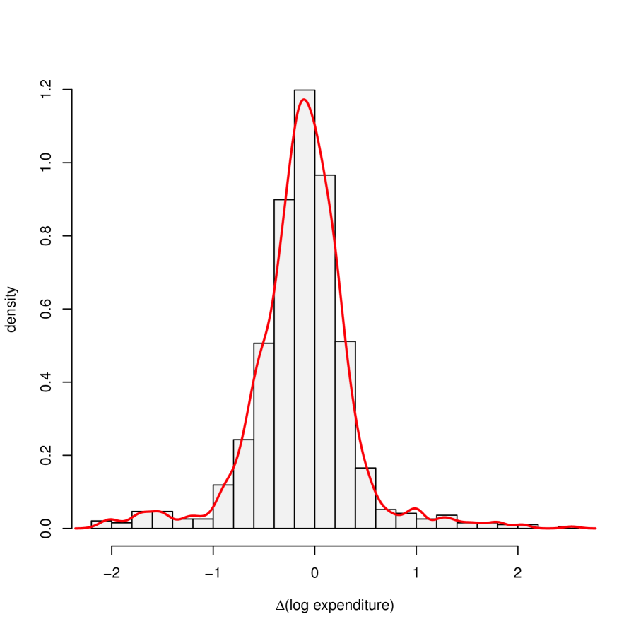
Figure 1: Density of the change in log-expenditure between 2007 and 2009.

Table 1 reports descriptive statistics for the variables used in the analysis. Both total expenditure and expenditure shares display within and between household variation, with means and standard deviations that remain stable between 2007 and 2009. The low percentage of within variation in expenditure indicates that there might be a substantial number of households with zero or little change in expenditure across years. Figure 1 plots histogram and kernel estimates of the density of the change in expenditure between 2007 and 2009. The kernel estimates are obtained using a Gaussian kernel with Silverman’s rule of thumb for the bandwidth. The estimates confirm that there is a high density of households with zero change in expenditure. Our methods will identify mean and quantile effects for these households with $X_{i1}=X_{i2}$.

Table 1: Descriptive Statistics

	Pooled sample			2007 sample		2009 sample
Variable	Mean	Std. Dev.	Within (%)	Mean	Std. Dev.	Mean	Std. Dev.
Log expenditure	10.13	0.56	21	10.19	0.57	10.07	0.55
Food share	0.19	0.10	28	0.19	0.10	0.20	0.10
Leisure Share	0.10	0.10	26	0.10	0.09	0.10	0.10
Note: the source of the data is the PSID. The number of observations is 968 observations for each year.

We estimate the location time effects, scale time effects, conditional mean effects, and conditional quantile effects using sample analogs of the expressions in Theorems 4 and 5. In particular, we estimate the conditional expectation, variance, and quantile functions by the nonparametric series methods described in Section 6. We consider two different specifications for the series basis in all the estimators: a quadratic orthogonal polynomial and a cubic B-spline with three knots at the minimum, median and maximum of total log-expenditure in the data set. Both specifications are additively separable in the total log-expenditures of 2007 and 2009. We also compute cross sectional estimates that do not account for endogeneity. They are obtained by averaging the nonparametric series estimates in 2007 and 2009 that use the same specification of series basis as the panel estimates but only condition on contemporaneous expenditure. For inference, we construct 90% confidence bands around the estimates by weighted bootstrap with exponential weights and 499 repetitions. These bands are uniform in that they cover the entire function of interest with 90% probability asymptotically.

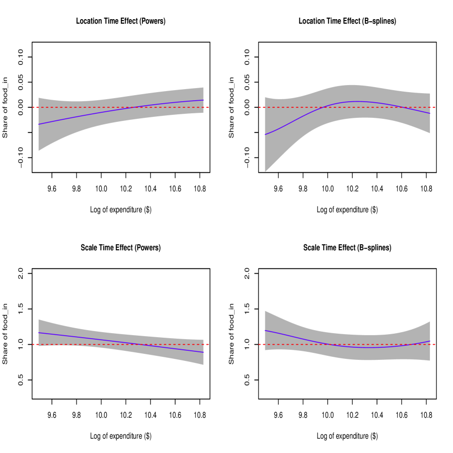
Figure 2: Location and scale time effects for food at home share: estimates from conditional quantiles.

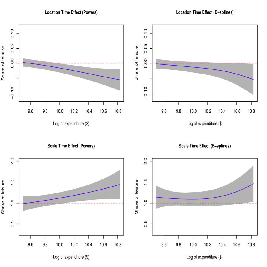
Figure 3: Location and scale time effects for leisure share: estimates from conditional quantiles.

Figures 2 and 3 show the estimates and confidence bands for the time effects functions:

$$x\mapsto\mu_{2}(x)-\mu_{1}(x)\sigma(x),\ \ x\mapsto\sigma(x)=\sigma_{2}(x)/\sigma_{1}(x),\ \ x\in\mathcal{X},$$

based on Theorem 5 with $\tau_{1}=.9,$ $\tau_{2}=.1,$ and $\tau_{3}=.5$, where $\mathcal{X}$ is the interval of values between the 0.10 and 0.90 sample quantiles of log-total expenditure. We find that we cannot reject the hypothesis that there are no location and scale time effects for food at home, whereas we find significant evidence of time effects for leisure with both series specifications. In results not reported, we find similar estimates and confidence bands for the time effects functions based on conditional means and variances using Theorem 4.

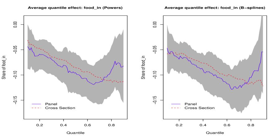
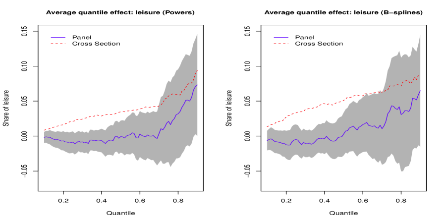
Figure 4: Average conditional quantile effects of log total expenditure.

Figure 4 plots the estimates and confidence bands for the time-averaged conditional quantile effects or CQSF derivates integrated over the values of $x$:

$$\tau\mapsto\int\left\{\bar{\mu}(x)+\partial_{x}\bar{\sigma}(x)q(\tau,x)+\bar{\sigma}(x)E[\partial_{x}\phi(x,U_{it})\mid\phi(x,U_{it})=q(\tau,x),X_{i1}=X_{i2}=x]\right\}\mu(dx),$$

for $\tau\in\mathcal{T},$ where $\mu$ is the empirical measure of log-expenditure, and $\mathcal{T}=[0.1,0.9].$ Here we find heterogeneity in the Engel curve relationship across the distribution. The pattern of the effect is increasing with the quantile index for both food at home and leisure, although the estimates are not sufficiently precise to distinguish these patterns from sampling noise. The cross sectional estimates plotted in dashed lines lie outside the confidence band for leisure, indicating significant evidence of endogeneity. We do not find such evidence for food at home.

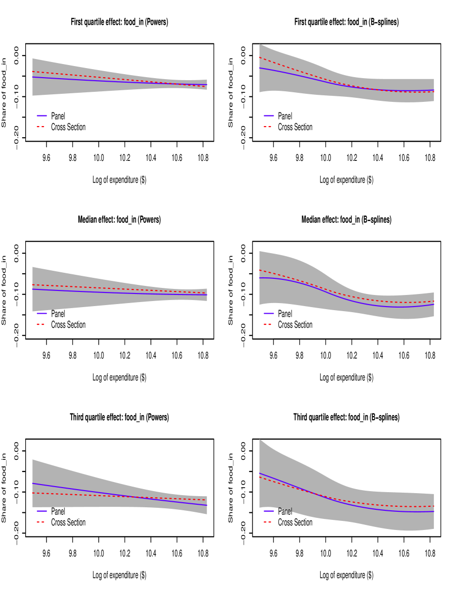
Figure 5: Conditional quartile effects of log total expenditure on food at home share.

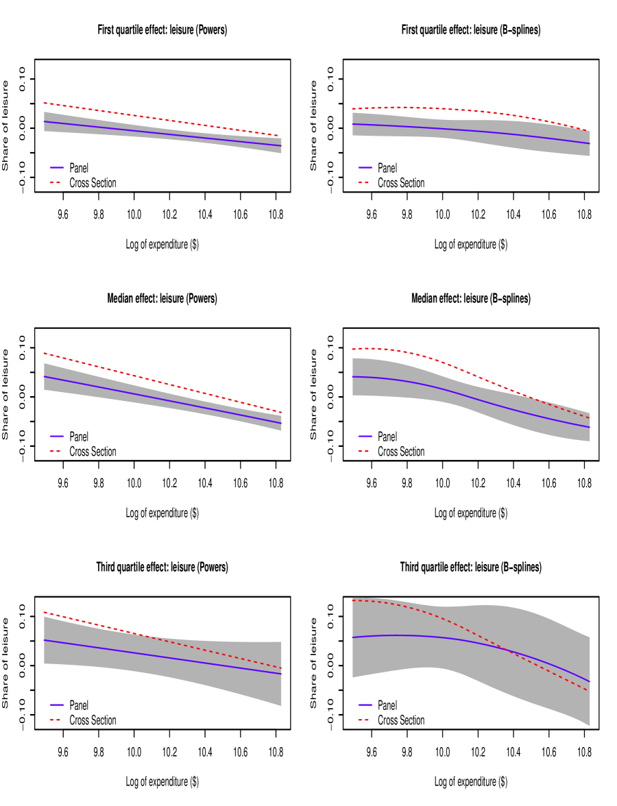
Figure 6: Conditional quartile effects of log total expenditure on leisure share.

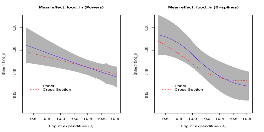
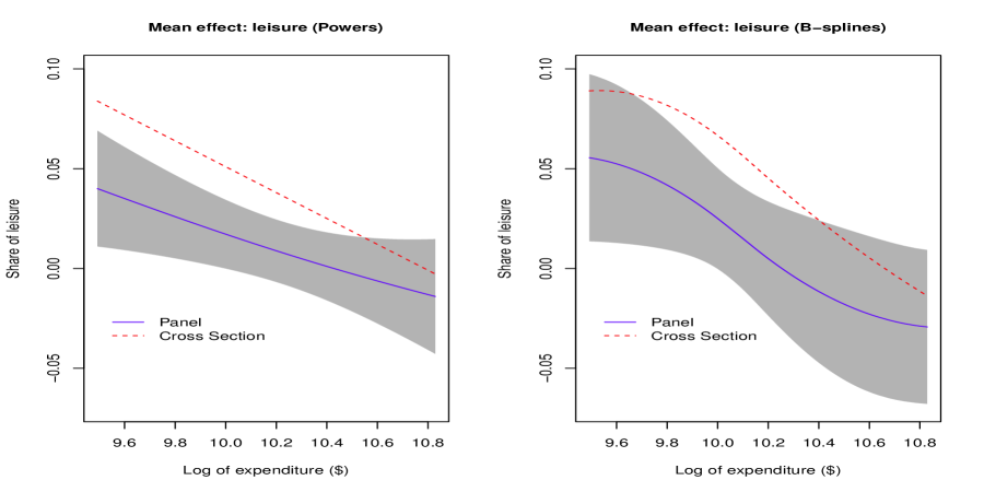
Figure 7: Conditional mean effects of log total expenditure.

In figures 5 and 6, we show that the panel estimates of the CQSF as a function of expenditure are decreasing for food at home and increasing for leisure at low values of expenditure. Imbens and Newey (2009) and Chen and Pouzo (2009, 2013) found similar patterns in their estimates of the QSF and the quantile Engel curves, respectively. Figure 7 plots the estimates and confidence bands for the time-averaged conditional mean effects or CASF derivatives:

$$x\mapsto\partial_{x}\bar{\mu}(x)+\partial_{x}\bar{\sigma}(x)E[\phi(x,U_{it})\mid X_{i1}=X_{i2}=x]+\bar{\sigma}(x)E[\partial_{x}\phi(x,U_{it})\mid X_{i1}=X_{i2}=x],\ \ x\in\mathcal{X}.$$

We also again evidence of endogeneity for leisure in the mean effects, but not for food at home. As in Blundell, Chen and Kristensen (2007), the conditional ASF is decreasing in expenditure for food at home, whereas it is increasing for leisure. We find that the curve is convex for food at home and concave for leisure. Note, however, that we should interpret the shape of our panel estimates with caution because they formally correspond to multiple conditional QSFs and ASFs as the conditioning set $X_{1}=X_{2}=x$ changes with $x$ along the curve.

Overall, the empirical results show that our panel estimates of the Engel curves are similar to previous cross sectional estimates based on IV methods to deal with endogeneity. Thus, the Engel curve relationship is decreasing for food at home and increasing for leisure. Moreover, we find evidence of the presence of time effects and endogeneity for leisure, but not for food at home. These finding are consistent with consumer preferences where food at home is a necessity good with little effect on the marginal allocation of income between consumption and savings. Leisure, on the other hand, is a superior good that affects the marginal allocation of income between consumption and savings. The Engel curve relationship is stable over time for food at home, whereas it is sensitive to changes over time in preferences and relative prices for leisure.

Appendix A Proof of Theorem 1

It follows from the differentiability of $\phi(x,u)$ and $f(u|x_{1},x_{2})$ and the dominance condition that

$$\tilde{M}(x,x_{1},x_{2}):=\int\phi(x,u)f(u|x_{1},x_{2})du$$

is continuously differentiable in $(x^{\prime},x_{1}^{\prime},x_{2}^{\prime})^{\prime}$ in a neighborhood of $(x^{\prime},x^{\prime},x^{\prime})$, and that the order of differentiation and integration can be interchanged. Furthermore, by the structure of the model and Assumption 2, for ${\boldsymbol{x}}=(x_{1}^{\prime},x_{2}^{\prime})^{\prime}$,

$$M_{t}({\boldsymbol{x}})=E\big{(}\phi(X_{t},U_{t})|X_{1}=x_{1},X_{2}=x_{2}\big{)}=\tilde{M}(x_{t},x_{1},x_{2}).$$

Therefore, $M_{t}({\boldsymbol{x}})$ is continuously differentiable in ${\boldsymbol{x}},$ $t=1,2,$ in a neighborhood of $(x^{\prime},x^{\prime})^{\prime}$, and for $s=1,2$,

$$\begin{split}\partial_{x_{s}}M_{t}({\boldsymbol{x}})&=\big{(}1(s=t)\partial_{x}\tilde{M}(x,x_{1},x_{2})+\partial_{x_{s}}\tilde{M}(x,x_{1},x_{2})\big{)}\big{|}_{(x,x_{1},x_{2})=(x_{t},x_{1},x_{2})}\\ &=\int\big{(}1(s=t)\partial_{x}\phi(x_{t},u)f(u|{\boldsymbol{x}})+\phi(x_{t},u)\partial_{x_{s}}f(u|{\boldsymbol{x}})\big{)}du\\ &=E\Big{(}\big{(}1(s=t)\partial_{x}\phi(x_{t},U_{t})+\phi(x_{t},U_{t})h_{s}(U_{t}|{\boldsymbol{x}})\big{)}\big{|}{\boldsymbol{X}}={\boldsymbol{x}}\Big{)},\end{split}$$ (A.1)

where $h_{s}(u|x)=f(u|{\boldsymbol{x}})^{-1}\partial_{x_{s}}f(u|{\boldsymbol{x}})$. Subtracting and using $U_{1}|{\boldsymbol{X}}\overset{d}{=}U_{2}|{\boldsymbol{X}}$,

$$\partial_{x_{2}}M_{2}({\boldsymbol{x}})-\partial_{x_{2}}M_{1}({\boldsymbol{x}}) =E\big{(}\partial_{x}\phi(x_{2},U_{2})\big{|}{\boldsymbol{X}}={\boldsymbol{x}}\big{)}$$

$$+E\Big{(}\big{(}\phi(x_{2},U_{2})-\phi(x_{1},U_{2})\big{)}\,h_{2}(U_{2}|{\boldsymbol{x}})\big{)}\big{|}{\boldsymbol{X}}={\boldsymbol{x}}\Big{)}.$$

Evaluating at ${\boldsymbol{x}}=(x^{\prime},x^{\prime})^{\prime}$ gives (2.2), and (2.3) follows similarly by considering $\partial_{x_{1}}M_{1}({\boldsymbol{x}})-\partial_{x_{1}}M_{2}({\boldsymbol{x}})$, using (A.1) and evaluating at ${\boldsymbol{x}}=(x^{\prime},x^{\prime})^{\prime}$. ∎

Appendix B Proof of Lemma 1

Let $F_{E}(e|h,{\boldsymbol{x}})=\mathbb{P}(E\leq e|H=h,{\boldsymbol{X}}={\boldsymbol{x}})=\int_{-\infty}^{e}f_{E}(\epsilon|h,{\boldsymbol{x}})\,d\epsilon.$ Then by the fundamental theorem of calculus, $F_{E}(e|h,{\boldsymbol{x}})$ is differentiable in $e$ with derivative $f_{E}(e|h,{\boldsymbol{x}})$ that is continuous in $e$ and ${\boldsymbol{x}}$. Consider

$$\begin{split}&\mathbb{P}(\phi(x,U_{t})\leq y|{\boldsymbol{X}}={\boldsymbol{x}})=\int 1(\phi(x,u)\leq y)\,f(u|{\boldsymbol{x}})\,du\\ &=\int\int 1(\phi(x,h,e)\leq y)\,f_{E}(e|h,{\boldsymbol{x}})\,f(h|{\boldsymbol{x}})de\,dh\\ &=\int\int 1(e\leq\phi^{-1}(x,h,y))\,f_{E}(e|h,{\boldsymbol{x}})\,f(h|{\boldsymbol{x}})de\,dh\\ &=\int F_{E}(\phi^{-1}(x,h,y)|h,{\boldsymbol{x}})f(h|{\boldsymbol{x}})\,dh.\end{split}$$ (B.1)

By the inverse and implicit function theorems, $\phi^{-1}(x,h,y)$ is continuously differentiable in $x$ and $y,$ with

$$\partial_{y}\phi^{-1}(x,h,y) = \big{[}\partial_{e}\phi(x,h,\phi^{-1}(x,h,y))\big{]}^{-1},$$

$$\partial_{x}\phi^{-1}(x,h,y) = -\frac{\partial_{x}\phi(x,h,\phi^{-1}(x,h,y))}{\partial_{e}\phi(x,h,\phi^{-1}(x,h,y))}$$

$$= -\partial_{x}\phi(x,h,\phi^{-1}(x,h,y))\,\partial_{y}\phi^{-1}(x,h,y).$$

Then by Assumption 3 both $\partial_{y}\phi^{-1}(x,h,y)$ and $\partial_{x}\phi^{-1}(x,h,y)$ are continuous in $y$ and $x$ and bounded. Therefore,

$$\begin{split}\partial_{y}F_{E}(\phi^{-1}(x,h,y)|h,{\boldsymbol{x}})&=f_{E}(\phi^{-1}(x,h,y)|h,{\boldsymbol{x}})\,\partial_{y}\phi^{-1}(x,h,y)\\ &=f_{Y_{x}|{\boldsymbol{X}},H_{t}}(y|{\boldsymbol{x}},h),\\ \partial_{x}F_{E}(\phi^{-1}(x,h,y)|h,{\boldsymbol{x}})&=f_{E}(\phi^{-1}(x,h,y)|h,{\boldsymbol{x}})\,\partial_{x}\phi^{-1}(x,h,y)\\ &=-f_{Y_{x}|{\boldsymbol{X}},H_{t}}(y|{\boldsymbol{x}},h)\,\partial_{x}\phi(x,h,\phi^{-1}(x,h,y)),\end{split}$$ (B.2)

are both bounded and continuous in $y,x$ and ${\boldsymbol{x}},$ where the last equality in each equation follows by a standard change of variables argument. From the boundedness assumptions on $f_{E}$ and on $\partial_{x}\phi$ in Assumption 3, it follows that $\mathbb{P}(\phi(x,U_{t})\leq y|{\boldsymbol{X}}={\boldsymbol{x}})$ is partially differentiable in $y$ and $x$ with partial derivatives continuous in $y,x,{\boldsymbol{x}}$, which can be computed by differentiating under the integral in (B.1). In order to establish the expressions in the lemma, insert (B.2) into the partial derivatives of (B.1) w.r.t. $y$ and $x$, and note that $f_{Y_{x}|{\boldsymbol{X}},H_{t}}(y|{\boldsymbol{x}},h)f(h|{\boldsymbol{x}})=f_{Y_{x},H_{t}|{\boldsymbol{X}}}(y,h|{\boldsymbol{x}})$. The first expression is then immediate. For the second, note that given $Y_{x}=y$ (for a fixed $x$), $E_{t}=\phi^{-1}(x,H_{t},y)$, so that

$$f_{Y_{x}|{\boldsymbol{X}}}(y|{\boldsymbol{x}})\,E\big{(}\partial_{x}\phi(x,U_{t})|Y_{x}=y,{\boldsymbol{X}}={\boldsymbol{x}}\big{)}$$

$$= f_{Y_{x}|{\boldsymbol{X}}}(y|{\boldsymbol{x}})\,\int\partial_{x}\phi(x,h,\phi^{-1}(x,h,y))\,f_{H_{t}|Y_{x},{\boldsymbol{X}}}(h|y,{\boldsymbol{x}})\,dh$$

$$= \int\partial_{x}\phi(x,h,\phi^{-1}(x,h,y))\,f_{Y_{x},H_{t}|{\boldsymbol{X}}}(y,h|{\boldsymbol{x}})\,dh.$$

∎

Appendix C Proof of Theorem 2

Let ${\boldsymbol{z}}=(y,x^{\prime},{\boldsymbol{x}}^{\prime})^{\prime}$ and let $H({\boldsymbol{z}})=\mathbb{P}(\phi(x,U_{t})\leq y|{\boldsymbol{X}}={\boldsymbol{x}})$. From Lemma 1 it follows that $H({\boldsymbol{z}})$ is differentiable in $y$ and $x$ with partial derivatives continuous in ${\boldsymbol{z}}$.

From (3.3), it follows that $H({\boldsymbol{z}})$ is also differentiable in ${\boldsymbol{x}}$ with

$$\partial_{\boldsymbol{x}}H({\boldsymbol{z}})=\int 1(\phi(x,u)\leq y)\partial_{\boldsymbol{x}}f(u|{\boldsymbol{x}})du$$

which is continuous in ${\boldsymbol{z}}$. Thus, $H({\boldsymbol{z}})$ is continuously differentiable in ${\boldsymbol{z}}$, and the derivative w.r.t. $y$ is strictly positive (see the expression in Lemma 1). From the implicit function theorem, there is a unique solution $Q_{t}(\tau|{\boldsymbol{x}})$, ${\boldsymbol{x}}=(x_{1}^{\prime},x_{2}^{\prime})^{\prime}$, to

$$\tau=H(Q_{t}(\tau|{\boldsymbol{x}}),x_{t},{\boldsymbol{x}}),\qquad t=1,2.$$

which is differentiable with partial derivatives

$$\partial_{x_{s}}Q_{t}(\tau|{\boldsymbol{x}})=-\big{(}\partial_{y}H(Q_{t}(\tau|{\boldsymbol{x}}),x_{t},{\boldsymbol{x}})\big{)}^{-1}\,\Big{(}1(s=t)\partial_{x}H(Q_{t}(\tau|{\boldsymbol{x}}),x_{t},{\boldsymbol{x}})+\partial_{x_{s}}H(Q_{t}(\tau|{\boldsymbol{x}}),x_{t},{\boldsymbol{x}})\Big{)},$$

where $\partial_{x_{s}}H\big{(}y,x,{\boldsymbol{x}})$ is the partial derivative w.r.t. the components of $x_{s}$ in ${\boldsymbol{x}}=(x_{1}^{\prime},x_{2}^{\prime})^{\prime}$, $s=1,2$. Evaluating at $x_{1}=x_{2}=x$, subtracting and plugging in the expressions for the derivatives from Lemma 1 yields (3.1). ∎

Appendix D Proof of Proposition 1

Fix $x_{1}$, and set

$$H(y,x_{2})=P(Y\leq y|X_{1}=x_{1},X_{2}=x_{2})=P(g(x_{1},x_{2},{\boldsymbol{U}})\leq y|X_{1}=x_{1})$$

by the form of the model and the conditional independence assumption. Below we show that from Assumption 5, $H(y,x_{2})$ is continuously partially differentiable with derivatives

$$\begin{split}\partial_{y}H(y,x_{2})&=f_{Y|X_{1},X_{2}}(y|x_{1},x_{2}),\\ \partial_{x_{2}}H(y,x_{2})&=-f_{Y|X_{1},X_{2}}(y|x_{1},x_{2})\,E\big{(}\partial_{x_{2}}g(X_{1},X_{2},{\boldsymbol{U}})|Y=y,X_{1}=x_{1},X_{2}=x_{2}\big{)}.\end{split}$$ (D.1)

From the positivity of the conditional density of $Y$ given $X_{1},X_{2}$ and the implicit function theorem, the conditional quantile $q(\tau,x_{1},x_{2})$ given by $H\big{(}q(\tau,x_{1},x_{2}),x_{2}\big{)}=\tau$ exists and is differentiable in $x_{2}$ with derivative

$$\partial_{x_{2}}q(\tau,x_{1},x_{2}) =-\Big{(}\partial_{y}H\big{(}q(\tau,x_{1},x_{2}),x_{2}\big{)}\Big{)}^{-1}\partial_{x_{2}}H\big{(}q(\tau,x_{1},x_{2}),x_{2}\big{)}$$

$$=E\big{(}\partial_{x_{2}}g(X_{1},X_{2},{\boldsymbol{U}})|Y=q(\tau,x_{1},x_{2}),X_{1}=x_{1},X_{2}=x_{2}\big{)}.$$

where we used (D.1), thus proving the theorem.

It remains to prove (D.1), which is analogous to Lemma 1. Let $F_{E}(e|h,{\boldsymbol{x}})=\mathbb{P}(E\leq e|H=h,X_{1}=x_{1})=\int_{-\infty}^{e}f_{E}(e|h,x_{1})\,de$, so that $F_{E}(e|h,x_{1})$ is differentiable in $e$ with derivative $f_{E}(e|h,x_{1})$ that is continuous in $e$. Consider

$$\begin{split}&\mathbb{P}(g(x_{1},x_{2},{\boldsymbol{U}})\leq y|X_{1}=x_{1})=\int 1(g(x_{1},x_{2},{\boldsymbol{u}})\leq y)\,f({\boldsymbol{u}}|x_{1})\,du\\ &=\int\int 1(g(x_{1},x_{2},h,e)\leq y)\,f_{E}(e|h,x_{1})\,f(h|x_{1})de\,dh\\ &=\int\int 1(e\leq g^{-1}(x_{1},x_{2},h,y))\,f_{E}(e|h,x_{1})\,f(h|x_{1})de\,dh\\ &=\int F_{E}(g^{-1}(x_{1},x_{2},h,y)|h,x_{1})f(h|x_{1})\,dh.\end{split}$$ (D.2)

By the inverse and implicit function theorems, $g^{-1}(x_{1},x_{2},h,y)$ is continuously differentiable in $x$ and $y,$ with

$$\partial_{y}\big{(}g^{-1}(x_{1},x_{2},h,y)\big{)} = \big{(}\partial_{e}g(x_{1},x_{2},h,g^{-1}(x_{1},x_{2},h,y))\big{)}^{-1},$$

$$\partial_{x_{2}}\big{(}g^{-1}(x_{1},x_{2},h,y)\big{)} = -\frac{\partial_{x_{2}}g(x_{1},x_{2},h,g^{-1}(x_{1},x_{2},h,y))}{\partial_{e}g(x_{1},x_{2},h,g^{-1}(x_{1},x_{2},h,y))}$$

$$= -\partial_{x_{2}}g(x_{1},x_{2},h,g^{-1}(x_{1},x_{2},h,y))\,\partial_{y}\big{(}g^{-1}(x_{1},x_{2},h,y)\big{)}.$$

Then by Assumption 5 both $\partial_{y}\big{(}g^{-1}(x_{1},x_{2},h,y)\big{)}$ and $\partial_{x_{2}}\big{(}g^{-1}(x_{1},x_{2},h,y)\big{)}$ are continuous in $y$ and $x_{2}$ and bounded. Therefore,

$$\begin{split}\partial_{y}\big{(}F_{E}(g^{-1}(x_{1},x_{2},h,y)|h,x_{1})\big{)}&=f_{E}(g^{-1}(x_{1},x_{2},h,y)|h,x_{1})\,\partial_{y}\big{(}g^{-1}(x_{1},x_{2},h,y)\big{)}\\ &=f_{Y|X_{1},X_{2},H}(y|x_{1},x_{2},h),\\ \partial_{x_{2}}\big{(}F_{E}(g^{-1}(x_{1},x_{2},h,y)|h,{\boldsymbol{x}})\big{)}&=f_{E}(g^{-1}(x_{1},x_{2},h,y)|h,{\boldsymbol{x}})\,\partial_{x_{2}}\big{(}g^{-1}(x_{1},x_{2},h,y)\big{)}\\ &=-f_{Y|X_{1},X_{2},H}(y|x_{1},x_{2},h)\,\partial_{x_{2}}g(x_{1},x_{2},h,g^{-1}(x_{1},x_{2},h,y)),\end{split}$$ (D.3)

are both bounded and continuous in $y,x$ and ${\boldsymbol{x}},$ where the last equality in each equation follows by a change of variables argument together with conditional independence of $X_{2}$ and $(H,E)$ given $X_{1}$. From the boundedness assumptions on $f_{E}$ and on $\partial_{x_{2}}g$ in Assumption 5, it follows that $H(y,x_{2})$ is partially differentiable with continuous partial derivatives which can be computed by differentiating under the integral in (D.2). Now insert (D.3) into (D.2) and note that $f_{Y|X_{1},X_{2},H}(y|x_{1},x_{2},h)f(h|x_{1})=f_{Y,H|X_{1},X_{2}}(y,h|x_{1},x_{2})$ by conditional independence. The first expression is then immediate. For the second, note that given $Y=y$ (for a fixed $x_{1},x_{2}$), $E=g^{-1}(x_{1},x_{2},H,y)$, so that

$$f_{Y|X_{1},X_{2}}(y|x_{1},x_{2})\,E\big{(}\partial_{x_{2}}g(x_{1},x_{2},{\boldsymbol{U}})|Y=y,X_{1}=x_{1},X_{2}=x_{2}\big{)}$$

$$= f_{Y|X_{1},X_{2}}(y|x_{1},x_{2})\,\int\partial_{x_{2}}g(x_{1},x_{2},h,g^{-1}(x_{1},x_{2},h,y))\,f_{H|Y,X_{1},X_{2}}(h|y,x_{1},x_{2})\,dh$$

$$= \int\partial_{x_{2}}g(x_{1},x_{2},h,g^{-1}(x_{1},x_{2},h,y))\,f_{Y,H|X_{1},X_{2}}(y,h|x_{1},x_{2})\,dh.$$

∎

Appendix E Proof of Theorem 4

The first result follows by direct calculation because

$$V_{t}(x,x)=\sigma_{t}^{2}(x)\text{Var}[\phi(x,U_{t})\mid X_{1}=X_{2}=x],$$

and $\text{Var}[\phi(x,U_{t})\mid X_{1}=X_{2}=x]$ does not depend on $t$ by Assumption 2.

For the second result, note that

$$E[Y_{2}-\sigma(x)Y_{1}\mid X_{1}=X_{2}=x]=M_{2}(x,x)-\sigma(x)M_{1}(x,x).$$

Then the result follows by direct calculation because

$$M_{t}(x,x)=\mu_{t}(x)+\sigma_{t}(x)E[\phi(x,U_{t})\mid X_{1}=X_{2}=x],\ \$$

and $E[\phi(x,U_{t})\mid X_{1}=X_{2}=x]$ does not depend on $t$ by Assumption 2.

The proof of the third result is similar to the proof of Theorem 1 replacing $\phi(x,u)$ by $\phi_{t}(x,u)=\mu_{t}(x)+\sigma_{t}(x)\phi(x,u)$. In particular, ${\boldsymbol{x}}\mapsto M_{t}({\boldsymbol{x}})$ is continuously differentiable, $t=1,2$, in a neighborhood of $(x^{\prime},x^{\prime})^{\prime},$ and for $s=1,2,$

$$\partial_{x_{s}}M_{t}({\boldsymbol{x}})=E\Big{(}1(s=t)\partial_{x}\phi_{t}(x_{t},U_{t})+\sigma_{t}(x_{t})\phi(x_{t},U_{t})h_{s}(U_{t}|{\boldsymbol{x}})\big{|}{\boldsymbol{X}}={\boldsymbol{x}}\Big{)},$$

where $h_{s}(u|{\boldsymbol{x}})=f(u|{\boldsymbol{x}})^{-1}\partial_{x_{s}}f(u|{\boldsymbol{x}})$ and $\partial_{x}\phi_{t}(x,u)=\partial_{x}\mu_{t}(x)+\partial_{x}\sigma_{t}(x)\phi(x,u)+\sigma_{t}(x)\partial_{x}\phi(x,u)$. Subtracting and using Assumption 2,

$$\partial_{x_{2}}M_{2}({\boldsymbol{x}})-\sigma(x)\partial_{x_{2}}M_{1}({\boldsymbol{x}}) =E\big{(}\partial_{x}\phi_{t}(x_{2},U_{2})\big{|}{\boldsymbol{X}}={\boldsymbol{x}}\big{)}$$

$$+E\Big{(}\big{(}\sigma_{2}(x_{2})\phi(x_{2},U_{2})-\sigma(x)\sigma_{1}(x_{1})\phi(x_{1},U_{2})\big{)}\,h_{2}(U_{2}|{\boldsymbol{x}})\big{)}\big{|}{\boldsymbol{X}}={\boldsymbol{x}}\Big{)}.$$

Evaluating at ${\boldsymbol{x}}=(x^{\prime},x^{\prime})^{\prime}$ gives

$$\partial_{x_{2}}M_{2}(x,x)-\sigma(x)\partial_{x_{2}}M_{1}(x,x)=E\big{(}\partial_{x}\phi_{2}(x,U_{2})\big{|}X_{1}=X_{2}=x\big{)}.$$

A similar argument yields

$$\partial_{x_{1}}M_{1}(x,x)-\partial_{x_{1}}M_{2}(x,x)/\sigma(x)=E\big{(}\partial_{x}\phi_{1}(x,U_{1})\big{|}X_{1}=X_{2}=x\big{)}.$$

The result follows by averaging the previous expressions and using that $E\big{(}\partial_{x}\phi(x,U_{t})\big{|}X_{1}=X_{2}=x\big{)}$ does not depend on $t$ by Assumption 2. ∎

Appendix F Proof of Theorem 5

Let ${\boldsymbol{z}}=(y,x^{\prime},{\boldsymbol{x}}^{\prime})^{\prime}$ and let $H_{t}({\boldsymbol{z}})=\mathbb{P}(\phi_{t}(x,U_{t})\leq y|{\boldsymbol{X}}={\boldsymbol{x}})$ where $\phi_{t}(x,u)=\mu_{t}(x)+\sigma_{t}(x)\phi(x,u)$. The first result follows by a similar argument to the proof of Theorem 2. In particular, by Lemma 1 and (5.1), ${\boldsymbol{z}}\mapsto H_{t}({\boldsymbol{z}})$ is continuously differentiable with derivatives

$$\partial_{y}H_{t}({\boldsymbol{z}}) =f_{\phi_{t}(x,U_{t})|{\boldsymbol{X}}}(y|{\boldsymbol{x}}),$$

$$\partial_{x}H_{t}({\boldsymbol{z}}) =-f_{\phi_{t}(x,U_{t})|{\boldsymbol{X}}}(y|{\boldsymbol{x}})E\big{(}\partial_{x}\phi_{t}(x,U_{t})|\phi_{t}(x,U_{t})=y,{\boldsymbol{X}}={\boldsymbol{x}}\big{)},$$

$$\partial_{\boldsymbol{x}}H({\boldsymbol{z}}) =\int 1(\phi_{t}(x,u)\leq y)\partial_{\boldsymbol{x}}f(u|{\boldsymbol{x}})du.$$

Thus, ${\boldsymbol{z}}\mapsto H_{t}({\boldsymbol{z}})$ is continuously differentiable with positive derivative with respect to $y$. By the implicit function theorem, there is a unique solution $Q_{t}(\tau|{\boldsymbol{x}})$ to $\tau=H_{t}(Q_{t}(\tau|{\boldsymbol{x}}),x_{t},{\boldsymbol{x}}),$ $t=1,2,$ which is differentiable with partial derivatives

$$\partial_{x_{s}}Q_{t}(\tau|{\boldsymbol{x}})=-\big{(}\partial_{y}H_{t}(Q_{t}(\tau|{\boldsymbol{x}}),x_{t},{\boldsymbol{x}})\big{)}^{-1}\,\Big{(}1(s=t)\partial_{x}H_{t}(Q_{t}(\tau|{\boldsymbol{x}}),x_{t},{\boldsymbol{x}})+\partial_{x_{s}}H_{t}(Q_{t}(\tau|{\boldsymbol{x}}),x_{t},{\boldsymbol{x}})\Big{)},$$

where $\partial_{x_{s}}H_{t}\big{(}y,x,{\boldsymbol{x}})$ is the partial derivative w.r.t. the components of $x_{s}$ in ${\boldsymbol{x}}=(x_{1}^{\prime},x_{2}^{\prime})^{\prime}$, $s=1,2$.

Evaluating at $x_{1}=x_{2}=x$, and plugging in the expressions for the derivatives yields

$$\partial_{x_{s}}Q_{t}(\tau|{\boldsymbol{x}})=1(s=t)E\big{(}\partial_{x}\phi_{t}(x,U_{t})|\phi(x,U_{t})=q(\tau,x),X_{1}=X_{2}=x\big{)}\\ -[f_{\phi(x,U_{t})|{\boldsymbol{X}}}(q(\tau,x)|{\boldsymbol{x}})/\sigma_{t}(x)]^{-1}\int 1(\phi(x,u)\leq q(\tau,x))\partial_{x_{s}}f(u|{\boldsymbol{x}})du,$$

where we use that $Q_{t}(\tau|{\boldsymbol{x}})=\mu_{t}(x)+\sigma_{t}(x)q(\tau,x)$ by invariance of quantiles to monotone transformations, and $f_{\phi_{t}(x,U_{t})|{\boldsymbol{X}}}(y|{\boldsymbol{x}})=f_{\phi(x,U_{t})|{\boldsymbol{X}}}([y-\mu_{t}(x)]/\sigma_{t}(x)|{\boldsymbol{x}})/\sigma_{t}(x)$ by a change of variables. Subtracting and using Assumption 2

$$\partial_{x_{1}}Q_{1}(\tau|{\boldsymbol{x}})-\sigma(x)^{-1}\partial_{x_{1}}Q_{2}(\tau|{\boldsymbol{x}})=E\big{(}\partial_{x}\phi_{1}(x,U_{1})|\phi(x,U_{1})=q(\tau,x),X_{1}=X_{2}=x\big{)},$$

and

$$\partial_{x_{2}}Q_{2}(\tau|{\boldsymbol{x}})-\sigma(x)\partial_{x_{2}}Q_{1}(\tau|{\boldsymbol{x}})=E\big{(}\partial_{x}\phi_{2}(x,U_{2})|\phi(x,U_{2})=q(\tau,x),X_{1}=X_{2}=x\big{)}.$$

The result then follows by averaging the previous expressions, using $\partial_{x}\phi_{t}(x,u)=\partial_{x}\mu_{t}(x)+\partial_{x}\sigma_{t}(x)\phi(x,u)+\sigma_{t}(x)\partial_{x}\phi(x,u)$ and that $E\big{(}\partial_{x}\phi(x,U_{t})|\phi(x,U_{t})=q(\tau,x),X_{1}=X_{2}=x\big{)}$ does not depend on $t$ by Assumption 2.

The second and third results follow from Assumption 2 by direct calculation because

$$Q_{t}(\tau\mid x,x)=\mu_{t}(x)+\sigma_{t}(x)q(\tau,x).$$

∎

References

• [1] Altonji, J., and R. Matzkin (2005): “Cross Section and Panel Data Estimators for Nonseparable Models with Endogenous Regressors”, Econometrica 73, 1053-1102.
• [2] Belloni, A., Chernozhukov, V., Chetverikov, D., and K. Kato (2013), “On the Asymptotic Theory for Least Squares Series: Pointwise and Uniform Results,” arXiv:1212:0442.
• [3] Belloni, A., Chernozhukov, V., and I. Fernandez-Val (2011), “Conditional quantile processes based on series or many regressors,” arXiv:1105.6154.
• [4] Bester, A.C., and C. Hansen (2009), “Identification of Marginal Effects in a Nonparametric Correlated Random Effects Model,” Journal of Business & Economic Statistics 27(2), pp. 235–250.
• [5] Browning, M. and J. Carro (2007), “Heterogeneity and Microeconometrics Modeling,” in Blundell, R., W.K. Newey, T. Persson (eds.), Advances in Theory and Econometrics, Vol. 3, Cambridge: Cambridge University Press.
• [6] Blundell, R., Chen, X., and D. Kristensen (2007)  “Semi-nonparametric IV Estimation of Shape-Invariant Engel Curves.” Econometrica 75(6). pp. 1613-1669.
• [7] Chamberlain, G. (1980), “Analysis of Covariance with Qualitative Data,” Review of Economic Studies, 47, pp. 225–238.
• [8] Chamberlain, G. (1982), “Multivariate Regression Models for Panel Data,” Journal of Econometrics, 18, 5–46.
• [9] Chamberlain, G. (1984), “Panel Data,” in Z. Griliches and M. Intriligator eds Handbook of Econometrics. Amsterdam: North-Holland.
• [10] Chamberlain, G., and G. W. Imbens (2003), “Nonparametric applications of Bayesian inference,” Journal of Business & Economic Statistics 21, 12–18.
• [11] Chen, X., and Pouzo, D. (2009)  “Efficient Estimation of Semiparametric Conditional Moment Models with Possibly Nonsmooth Residuals,” Journal of Econometrics, 152(1), 46-60.
• [12] Chen, X., and Pouzo, D. (2013)  “Sieve Quasi Likelihood Ratio Inference on Semi/nonparametric Conditional Moment Models,” Cowles Foundation Discussion Paper 1897.
• [13] Chernozhukov, V., Fernandez-Val, I., Hahn, J., and W. K. Newey (2013), “Average and Quantile Effects in Nonseparable Panel Models,” Econometrica, 81(2), pp. 535–580.
• [14] Chernozhukov, V., Lee, S., and A.M. Rosen (2013), “Intersection bounds: estimation and inference,” Econometrica, 81 (2), pp. 667–737.
• [15] Evdokimov, K. (2010), “Identification and Estimation of a Nonparametric Panel Data Model with Unobserved Heterogeneity,” unpublished manuscript, Princeton University.
• [16] Fan, J. and Q. Yao (1998), “Efficient estimation of conditional variance functions in stochastic regression,” Biometrika, 85, pp. 645–660.
• [17] Graham, B.W. and J.L. Powell (2012), “Identification and Estimation of Average Partial Effects in “Irregular” Correlated Random Coefficient Panel Data Models,” Econometrica 80 (5), pp. 2105–2152.
• [18] Hahn, J. (1995), “Bootstrapping quantile regression estimators,”Econometric Theory 11, 105–121.
• [19] Hoderlein, S., and E. Mammen (2007): “Identification of Marginal Effects in Nonseparable Models without Monotonicity,” Econometrica, 75, 1513 - 1519.
• [20] Hoderlein, S. and H. White, (2012), ‘Nonparametric identi cation in nonseparable panel data models with generalized fixed effects’, Journal of Econometrics 168, 300-314.
• [21] Honore, B.E. (1992): ”Trimmed Lad and Least Squares Estimation of Truncated and Censored Regression Models with Fixed Effects,” Econometrica 60, 533-565
• [22] Hsiao, C. (2003), Analysis of panel data. Second edition. Econometric Society Monographs, 34. Cambridge University Press, Cambridge.
• [23] Imbens, G. and W.K. Newey (2009),  ”Identification and Estimation of Triangular Simultaneous Equations Models Without Additivity,” Econometrica 77, 1481-1512.
• [24] Koenker R. and G. Bassett, (1978): “Regression Quantiles,” Econometrica 46, pp. 33–50.
• [25] Lewbel, A. (2006)  “Entry for the New Palgrave Dictionary of Economics, 2nd Edition.” Boston College. .
• [26] Ma, S., and Kosorok, M. (2005):  “Robust Semiparametric M-Estimation and the Weighted Bootstrap,”Journal of Multivariate Analysis, 96(1), 190-217.
• [27] Manski, C. (1987): “Semiparametric Analysis of Random Effects Linear Models From Binary Response Data,” Econometrica 55, 357-362.
• [28] Praestgaard, J., and J. A. Wellner. (1993) “Exchangeably weighted bootstraps of the general empirical process,” The Annals of Probability, 2053–2086.
Refer to caption