Universidade de Aveiro Departamento de Matemática                                                                   2013Universidade de Aveiro

Shakoor Pooseh

Métodos Computacionais no Cálculo das Variações e Controlo Óptimo Fraccionais
Computational Methods in the Fractional Calculus of Variations and Optimal Control

Universidade de Aveiro Departamento de Matemática                                                                   2013Universidade de Aveiro

Shakoor Pooseh

Métodos Computacionais no Cálculo das Variações e Controlo Óptimo Fraccionais
Computational Methods in the Fractional Calculus of Variations and Optimal Control

Tese de Doutoramento apresentada à Universidade de Aveiro para cumprimento dos requisitos necessários à obtenção do grau de Doutor em Matemática, Programa Doutoral em Matemática e Aplicações, PDMA 2009–2013, da Universidade de Aveiro e Universidade do Minho realizada sob a orientação científica do Prof. Doutor Delfim Fernando Marado Torres, Professor Associado com Agregação do Departamento de Matemática da Universidade de Aveiro e do Prof. Doutor Ricardo Miguel Moreira de Almeida, Professor Auxiliar do Departamento de Matemática da Universidade de Aveiro.

Universidade de Aveiro Departamento de Matemática                                                                   2013Universidade de Aveiro

Shakoor Pooseh

Métodos Computacionais no Cálculo das Variações e Controlo Óptimo Fraccionais
Computational Methods in the Fractional Calculus of Variations and Optimal Control

Ph.D. thesis submitted to the University of Aveiro in fulfilment of the requirements for the degree of Doctor of Philosophy in Mathematics, Doctoral Programme in Mathematics and Applications 2009–2013, of the University of Aveiro and University of Minho, under the supervision of Professor Delfim Fernando Marado Torres, Associate Professor with Habilitation and tenure of the Department of Mathematics of University of Aveiro and Professor Ricardo Miguel Moreira de Almeida, Assistant Professor of the Department of Mathematics of University of Aveiro.

o júri

Presidente

Prof. Doutor Artur Manuel Soares da Silva
Professor Catedrático da Universidade de Aveiro

Prof. Doutor Stéphane Louis Clain
Professor Associado com Agregação da Escola de Ciências da Universidade do Minho

Prof. Doutor Manuel Duarte Ortigueira
Professor Associado com Agregação da Faculdade de Ciências e Tecnologia da Universidade Nova de Lisboa

Prof. Doutor Delfim Fernando Marado Torres
Professor Associado com Agregação da Universidade de Aveiro (Orientador)

Prof. Doutora Ercília Cristina Costa e Sousa
Professora Auxiliar da Faculdade de Ciências e Tecnologia da Universidade de Coimbra

Prof. Doutora Maria Luísa Ribeiro dos Santos Morgado
Professora Auxiliar da Faculdade de Ciências e Tecnologia da Universidade de Trás-os-Montes e Alto Douro

Prof. Doutor Ricardo Miguel Moreira de Almeida
Professor Auxiliar da Universidade de Aveiro (Coorientador)

agradecimentos

Esta tese de doutoramento é o resultado da colaboração de muitas pessoas. Primeiro de tudo, Delfim F. M. Torres, o meu orientador, que me ajudou muito ao longo dos últimos anos, proporcionando uma dinâmica e amigável atmosfera, propícia à investigação. Foi também grande sorte da minha parte ter Ricardo Almeida como co-orientador, agindo não só nesse qualidade, mas também como um amigo e colega. Devo a estas duas pessoas muito de aluno para orientador.
A actividade científica só é possível por um efectivo apoio financeiro, que a Fundação Portuguesa para a Ciência e a Tecnologia (FCT), me forneceu através da bolsa de doutoramento SFRH/BD/33761/2009, no âmbito do Programa Doutoral em Matemática e Aplicações (PDMA) das Universidades de Aveiro e Minho. Além do apoio financeiro da FCT, ter sido membro do Grupo de Teoria Matemática dos Sistemas e Controlo do Centro de Investigação e Desenvolvimento em Matemática e Aplicações (CIDMA) teve um papel fundamental, que aqui realço.
A todos os que tiveram um efeito sobre minha vida de estudante de doutoramento, professores, funcionários e amigos, gostaria de expressar os meus sinceros agradecimentos. À minha família e esposa, fundamentais como suporte mental e moral, compreensão e tolerância, pelo muito que me ajudaram e por suportarem algum tipo de vício em trabalho e egoísmo.

acknowledgements

This thesis is the result of a collaboration of many people. First of all, Delfim F. M. Torres, my supervisor, that helped me a lot through these years by providing a dynamic, yet friendly, atmosphere for research. A great luck of mine is also having Ricardo Almeida, acting not only as my co-advisor, but also as a friend and colleague. I owe these two people much than a student to supervisors.
A scientific activity is only possible by a good financial support, which the Portuguese Foundation for Science and Technology (FCT)– Fundação para a Ciência e a Tecnologia– provided me through the Ph.D. fellowship SFRH/BD/33761/2009, within Doctoral Program in Mathematics and Applications (PDMA) of Universities of Aveiro and Minho. Besides financial support, a good research team has a crucial role, which is well provided by CIDMA, Center for Research and Development in Mathematics and Applications, that I deeply appreciate.
Together with all who had an effect on my studentship life, from teachers and staff to friends, I would like to express grateful thanks to my family and my wife whom mental and moral supports, understanding, and tolerance helped me a lot; let me to be some kind of workaholic, ignorant and selfish.

palavras-chave

Optimização e controlo, cálculo fraccional, cálculo das variações fraccional, controlo óptimo fraccional, condições necessários de optimalidade, métodos directos, métodos indirectos, aproximação numérica, estimação de erros, equações diferenciais fraccionais.

resumo

O cálculo das variações e controlo óptimo fraccionais são generalizações das correspondentes teorias clássicas, que permitem formulações e modelar problemas com derivadas e integrais de ordem arbitrária. Devido à carência de métodos analíticos para resolver tais problemas fraccionais, técnicas numéricas são desenvolvidas. Nesta tese, investigamos a aproximação de operadores fraccionais recorrendo a séries de derivadas de ordem inteira e diferenças finitas generalizadas. Obtemos majorantes para o erro das aproximações propostas e estudamos a sua eficiência. Métodos directos e indirectos para a resolução de problemas variacionais fraccionais são estudados em detalhe. Discutimos também condições de optimalidade para diferentes tipos de problemas variacionais, sem e com restrições, e para problemas de controlo óptimo fraccionais. As técnicas numéricas introduzidas são ilustradas recorrendo a exemplos.

keywords

Optimization and control, fractional calculus, fractional calculus of variations, fractional optimal control, fractional necessary optimality conditions, direct methods, indirect methods, numerical approximation, error estimation, fractional differential equations.

abstract

The fractional calculus of variations and fractional optimal control are generalizations of the corresponding classical theories, that allow problem modeling and formulations with arbitrary order derivatives and integrals. Because of the lack of analytic methods to solve such fractional problems, numerical techniques are developed. Here, we mainly investigate the approximation of fractional operators by means of series of integer-order derivatives and generalized finite differences. We give upper bounds for the error of proposed approximations and study their efficiency. Direct and indirect methods in solving fractional variational problems are studied in detail. Furthermore, optimality conditions are discussed for different types of unconstrained and constrained variational problems and for fractional optimal control problems. The introduced numerical methods are employed to solve some illustrative examples.

2010 Mathematics Subject Classification: 26A33, 34A08, 65D20, 33F05, 49K15, 49M25, 49M99.

Introduction

This thesis is devoted to the study of numerical methods in the calculus of variations and optimal control in the presence of fractional derivatives and/or integrals. A fractional problem of the calculus of variations and optimal control consists in the study of an optimization problem in which, the objective functional or constraints depend on derivatives and integrals of arbitrary, real or complex, orders. This is a generalization of the classical theory, where derivatives and integrals can only appear in integer orders. Throughout this thesis we will call the problems in the calculus of variations and optimal control, variational problems. If at least one fractional term exists in the formulation, it is called a fractional variational problem.

The theory started in 1996 with the works of Riewe, in order to better describe non-conservative systems in mechanics [106, 107]. The subject is now under strong development due to its many applications in physics and engineering, providing more accurate models of physical phenomena (see, e.g., [38, 37, 118, 10, 16, 27, 44, 45, 49, 52, 53, 85, 88, 89]).

In order to provide a better understanding, the classical theory of the calculus of variations and optimal control is discussed briefly in the beginning of this thesis in Chapter 1. Major concepts and notions are presented; key features are pointed out and some solution methods are detailed. There are two major approaches in the classical theory of calculus of variations to solve problems. In one hand, using Euler–Lagrange necessary optimality conditions, we can reduce a variational problem to the study of a differential equation. Hereafter, one can use either analytical or numerical methods to solve the differential equation and reach the solution of the original problem (see, e.g., [68]). This approach is referred as indirect methods in the literature.

On the other hand, we can tackle the functional itself, directly. Direct methods are used to find the extremizer of a functional in two ways: Euler’s finite differences and Ritz methods. In the Ritz method, we either restrict admissible functions to all possible linear combinations

$$x_{n}(t)=\sum_{i=1}^{n}\alpha_{i}\phi_{i}(t),$$

with constant coefficients $\alpha_{i}$ and a set of known basis functions $\phi_{i}$, or we approximate the admissible functions with such combinations. Using $x_{n}$ and its derivatives whenever needed, one can transform the functional to a multivariate function of unknown coefficients $\alpha_{i}$. By finite differences, however, we consider the admissible functions not on the class of arbitrary curves, but only on polygonal curves made upon a given grid on the time horizon. Using an appropriate discrete approximation of the Lagrangian, and substituting the integral with a sum, and the derivatives by appropriate approximations, we can transform the main problem to the optimization of a function of several parameters: the values of the unknown function on mesh points (see, e.g., [46]).

A historical review of fractional calculus comes next in Chapter 2. In general terms, the field that allows us to define integrals and derivatives of arbitrary real or complex order is called fractional calculus and can be seen as a generalization of ordinary calculus. A fractional derivative of order $\alpha>0$, when $\alpha=n$ is an integer, coincides with the classical derivative of order $n\in\mathbb{N}$, while a fractional integral is an n-fold integral. The origin of fractional calculus goes back to the end of the seventeenth century, though the main contributions have been made during the last few decades [115, 117]. Namely it has been proven to be a useful tool in engineering and optimal control problems (see, e.g., [30, 31, 62, 43, 72, 112]). Furthermore, during the last three decades, several numerical methods have been developed in the field of fractional calculus. Some of their advantages, disadvantages, and improvements, are given in [19].

There are several different definitions of fractional derivatives in the literature, such as Riemann–Liouville, Grünwald–Letnikov, Caputo, etc. They posses different properties: each one of those definitions has its own advantages and disadvantages. Under certain conditions, however, they are equivalent and can be used interchangeably. The Riemann–Liouville and Caputo are the most common for fractional derivatives, and for fractional integrals the usual one is the Riemann–Liouville definition.

After some introductory arguments of classical theories for variational problems and fractional calculus, the next step is providing the framework that is required to include fractional terms in variational problems and is shown in Chapter 3. In this framework, the fractional calculus of variations and optimal control are research areas under strong current development. For the state of the art, we refer the reader to the recent book [79], for models and numerical methods we refer to [26].

A fractional variational problem consists in finding the extremizer of a functional that depends on fractional derivatives and/or integrals subject to some boundary conditions and possibly some extra constraints. As a simple example one can consider the following minimization problem:

$$\begin{gathered}J[x(\cdot)]=\int_{a}^{b}L(t,x(t),{{}_{a}D_{t}^{\alpha}}x(t))dt\longrightarrow\min,\\ x(a)=x_{a},\quad x(b)=x_{b},\end{gathered}$$ (1)

that depends on the left Riemann–Liouville derivative, ${{}_{a}D_{t}^{\alpha}}$. Although this has been a common formulation for a fractional variational problem, the consistency of fractional operators and the initial conditions is questioned by many authors. For further readings we refer to [90, 91, 121] and references therein.

An Euler–Lagrange equation for this problem has been derived first in [106, 107] (see also [1]). A generalization of the problem to include fractional integrals, the transversality conditions and many other aspects can be found in the literature of recent years. See [16, 21, 79] and references therein. Indirect methods for fractional variational problems have a vast background in the literature and can be considered a well studied subject: see [1, 12, 21, 55, 63, 69, 86, 107] and references therein that study different variants of the problem and discuss a bunch of possibilities in the presence of fractional terms, Euler–Lagrange equations and boundary conditions. With respect to results on fractional variational calculus via Caputo operators, we refer the reader to [4, 11, 17, 55, 77, 84, 87] and references therein.

Direct methods, however, to the best of our knowledge, have got less interest and are not well studied. A brief introduction of using finite differences has been made in [106], which can be regarded as a predecessor to what we call here an Euler-like direct method. A generalization of Leitmann’s direct method can be found in [16], while [75] discusses the Ritz direct method for optimal control problems that can easily be reduced to a problem of the calculus of variations.

It is well-known that for most problems involving fractional operators, such as fractional differential equations or fractional variational problems, one cannot provide methods to compute the exact solutions analytically. Therefore, numerical methods are being developed to provide tools for solving such problems. Using the Grünwald–Letnikov approach, it is convenient to approximate the fractional differentiation operator, $D^{\alpha}$, by generalized finite differences. In [93] some problems have been solved by this approximation. In [40] a predictor-corrector method is presented that converts an initial value problem into an equivalent Volterra integral equation, while [70] shows the use of numerical methods to solve such integral equations. A good survey on numerical methods for fractional differential equations can be found in [50].

A numerical scheme to solve fractional Lagrange problems has been presented in [2]. The method is based on approximating the problem to a set of algebraic equations using some basis functions. See Chapter 4 for details. A more general approach can be found in [119] that uses the Oustaloup recursive approximation of the fractional derivative, and reduces the problem to an integer-order (classical) optimal control problem. A similar approach is presented in [63], using an expansion formula for the left Riemann–Liouville fractional derivative developed in [22, 23], to establish a new scheme to solve fractional differential equations.

The scheme is based on an expansion formula for the Riemann–Liouville fractional derivative. Here we introduce a generalized version of this expansion, in Chapter 5, that results in an approximation, for left Riemann–Liouville derivative, of the form

$${{}_{a}D_{t}^{\alpha}}x(t)\approx A(t-a)^{-\alpha}x(t)+B(t-a)^{1-\alpha}\dot{x}(t)-\sum_{p=2}^{N}C(\alpha,p)(t-a)^{1-p-\alpha}V_{p}(t),$$ (2)

with

$$\left\{\begin{array}[]{l}\dot{V}_{p}(t)=(1-p)(t-a)^{p-2}x(t)\\ V_{p}(a)=0,\end{array}\right.$$

where $p=2,\ldots,N$, and the coefficients $A=A(\alpha,N)$, $B(\alpha,N)$ and $C(\alpha,p)$ are real numbers depending on $\alpha$ and $N$. The number $N$ is the order of approximation. Together with a different expansion formula that has been used to approximate the fractional Euler–Lagrange equation in [21], we perform an investigation of the advantages and disadvantages of approximating fractional derivatives by these expansions. The approximations transform fractional derivatives into finite sums containing only derivatives of integer order [98].

We show the efficiency of such approximations to evaluate fractional derivatives of a given function in closed form. Moreover, we discuss the possibility of evaluating fractional derivatives of discrete tabular data. The application to fractional differential equations is also developed through some concrete examples.

The same ideas are extended to fractional integrals in Chapter 6. Fractional integrals appear in many different contexts, e.g., when dealing with fractional variational problems or fractional optimal control [10, 12, 53, 77, 85]. Here we obtain a simple and effective approximation for fractional integrals. We obtain decomposition formulas for the left and right fractional integrals of functions of class $C^{n}$ [95].

In this PhD thesis we also consider the Hadamard fractional integral and fractional derivative [97]. Although the definitions go back to the works of Hadamard in 1892 [61], this type of operators are not yet well studied and much exists to be done. For related works on Hadamard fractional operators, see [34, 35, 64, 65, 67, 105].

An error analysis is given for each approximation whenever needed. These approximations are studied throughout some concrete examples. In each case we try to analyze problems for which the analytic solution is available, so we can compare the exact and the approximate solutions. This approach gives us the ability of measuring the accuracy of each method. To this end, we need to measure how close we get to the exact solutions. We can use the $2$-norm for instance, and define an error function $E[x(\cdot),\tilde{x}(\cdot)]$ by

$$E=\|x(\cdot)-\tilde{x}(\cdot)\|_{2}=\left(\int_{a}^{b}[x(t)-\tilde{x}(t)]^{2}dt\right)^{\frac{1}{2}},$$ (3)

where $x(\cdot)$ is defined on a certain interval $[a,b]$.

Before getting into the usage of these approximations for fractional variational problems, we introduce an Euler-like discrete method, and a discretization of the first variation to solve such problems in Chapter 7. The finite differences approximation for integer-order derivatives is generalized to derivatives of arbitrary order and gives rise to the Grünwald–Letnikov fractional derivative. Given a grid on $[a,b]$ as $a=t_{0},t_{1},\ldots,t_{n}=b$, where $t_{i}=t_{0}+ih$ for some $h>0$, we approximate the left Riemann–Liouville derivative as

$${{}_{a}D_{t_{i}}^{\alpha}}x(t_{i})\simeq\frac{1}{h^{\alpha}}\sum_{k=0}^{i}\left(\omega_{k}^{\alpha}\right)x(t_{i}-kh),$$

where $\left(\omega_{k}^{\alpha}\right)=(-1)^{k}\binom{\alpha}{k}=\frac{\Gamma(k-\alpha)}{\Gamma(-\alpha)\Gamma(k+1)}$. The method follows the same procedure as in the classical theory. Discretizing the functional by a quadrature rule, integer-order derivatives by finite differences and substituting fractional terms by corresponding generalized finite differences, results in a system of algebraic equations. Finally, one gets approximate values of state and control functions on a set of discrete points [99].

A different direct approach for classical problems has been introduced in [59, 60]. It uses the fact that the first variation of a functional must vanish along an extremizer. That is, if $x$ is an extremizer of a given variational functional $J$, the first variation of $J$ evaluated at $x$, along any variation $\eta$, must vanish. This means that

$$J^{\prime}[x,\eta]=\int_{a}^{b}\left[\frac{\partial L}{\partial x}(t,x(t),{{}_{a}D_{t}^{\alpha}}x(t))\eta(t)+\frac{\partial L}{\partial{{}_{a}D_{t}^{\alpha}}x}(t,x(t),{{}_{a}D_{t}^{\alpha}}x(t)){{}_{a}D_{t}^{\alpha}}\eta(t)\right]\,dt=0.$$

With a discretization on time horizon and a quadrature for this integral, we obtain a system of algebraic equations. The solution to this system gives an approximation to the original problem [103].

Considering indirect methods in Chapter 8, we transform the fractional variational problem into an integer-order problem. The job is done by substituting the fractional term by the corresponding approximation in which only integer-order derivatives exist. The resulting classic problem, which is considered as the approximated problem, can be solved by any available method in the literature. If we substitute the approximation (2) for the fractional term in (1), the outcome is an integer-order constrained variational problem

$$J[x(\cdot)] \approx \int_{a}^{b}L\left(t,x(t),\frac{Ax(t)}{(t-a)^{\alpha}}+\frac{B\dot{x}(t)}{(t-a)^{\alpha-1}}-\sum_{p=2}^{N}\frac{C(\alpha,p)V_{p}(t)}{(t-a)^{p+\alpha-1}}\right)dt$$

$$= \int_{a}^{b}L^{\prime}\left(t,x(t),\dot{x}(t),V_{2}(t),\ldots,V_{N}(t)\right)dt\longrightarrow\min$$

subject to

$$\left\{\begin{array}[]{l}\dot{V}_{p}(t)=(1-p)(t-a)^{p-2}x(t)\\ V_{p}(a)=0,\end{array}\right.$$

with $p=2,\ldots,N$. Once we have a tool to transform a fractional variational problem into an integer-order one, we can go further to study more complicated problems. As a first candidate, we study fractional optimal control problems with free final time in Chapter 9. The problem is stated in the following way:

$$J[x,u,T]=\int_{a}^{T}L(t,x(t),u(t))\,dt+\phi(T,x(T))\longrightarrow\min,$$

subject to the control system

$$M\dot{x}(t)+N\;{{}^{C}_{a}D_{t}^{\alpha}}x(t)=f(t,x(t),u(t)),$$

and the initial boundary condition

$$x(a)=x_{a},$$

with $(M,N)\not=(0,0)$, and $x_{a}$ a fixed real number. Our goal is to generalize previous works on fractional optimal control problems by considering the end time $T$ free and the dynamic control system involving integer and fractional order derivatives. First, we deduce necessary optimality conditions for this new problem with free end-point. Although this could be the beginning of the solution procedure, the lack of techniques to solve fractional differential equations prevent further progress. Another approach consists in using the approximation methods mentioned above, thereby converting the original problem into a classical optimal control problem that can be solved by standard computational techniques [102].

In the 18th century, Euler considered the problem of optimizing functionals depending not only on some unknown function $x$ and some derivative of $x$, but also on an antiderivative of $x$ (see [51]). Similar problems have been recently investigated in [58], where Lagrangians containing higher-order derivatives and optimal control problems are considered. More generally, it has been shown that the results of [58] hold on an arbitrary time scale [81]. Here, in Chapter 10, we study such problems within the framework of fractional calculus. Minimize the cost functional

$$J[x]=\int_{a}^{b}L(t,x(t),{{}^{C}_{a}D_{t}^{\alpha}}x(t),{{}_{a}I_{x}^{\beta}}x(t),z(t))dx,$$

where the variable $z$ is defined by

$$z(t)=\int_{a}^{t}l(\tau,x(\tau),{{}^{C}_{a}D_{\tau}^{\alpha}}x(\tau),{{}_{a}I_{\tau}^{\beta}}x(\tau))d\tau,$$

subject to the boundary conditions

$$x(a)=x_{a}\quad\mbox{and}\quad x(b)=x_{b}.$$

Our main contribution is an extension of the results presented in [4, 58] by considering Lagrangians containing an antiderivative, that in turn depends on the unknown function, a fractional integral, and a Caputo fractional derivative.

Transversality conditions are studied, where the variational functional $J$ depends also on the terminal time $T$, $J[x,T]$. We also consider isoperimetric problems with integral constraints of the same type. Fractional problems with holonomic constraints are considered and the situation when the Lagrangian depends on higher order Caputo derivatives is studied. Other aspects such as the Hamiltonian formalism, sufficient conditions of optimality under suitable convexity assumptions on the Lagrangian, and numerical results with illustrative examples are described in detail [12].

Synthesis

Chapter 1 The calculus of variations and optimal control

In this part we review the basic concepts that have essential role in the understanding of the second and main part of this dissertation. Starting with the notion of the calculus of variations, and without going into details, we recall the optimal control theory as well and point out its variational approach together with main concepts, definitions, and some important results from the classical theory. A brief historical introduction to the fractional calculus is given afterwards. At the same time, we introduce the theoretical framework of the whole work, fixing notations and nomenclature. At the end, the calculus of variations and optimal control problems involving fractional operators are discussed as fractional variational problems.

1.1 The calculus of variations

Many authors trace the origins of the calculus of variations back to the ancient times, the time of Dido, Queen of Carthage. Dido’s problem had an intellectual nature. The question is to lie as much land as possible within a bull’s hide. Queen Dido intelligently cut the hide into thin strips and no one knows if she encircled the land using the line she made off the strips. As it is well-known nowadays, thanks to the modern calculus of variations, the solution to Dido’s problem is a circle [68]. Aristotle (384–322 B.C) expresses a common belief in his Physics that nature follows the easiest path that requires the least amount of effort. This is the main idea behind many challenges to solve real-world problems [29].

1.1.1 From light beams to the Brachistochrone problem

Fermat believed that “nature operates by means and ways that are easiest and fastest” [56]. Studying the analysis of refractions, he used Galileo’s reasoning on falling objects and claimed that in this case nature does not take the shortest path, but the one which has the least traverse time. Although the solution to this problem does not use variational methods, it has an important role in the solution of the most critical problem and the birth of the calculus of variations.

Newton also considered the problem of motion in a resisting medium, which is indeed a shape optimization problem. This problem is a well-known and well-studied example in the theory of the calculus of variations and optimal control nowadays [92, 113, 57]. Nevertheless, the original problem, posed by Newton, was solved by only using calculus.

In 1796-1797, John Bernoulli challenged the mathematical world to solve a problem that he called the Brachistochrone problem:

If in a vertical plane two points A and B are given, then it is required to specify the orbit AMB of the movable point M, along which it, starting from A, and under the influence of its own weight, arrives at B in the shortest possible time. So that those who are keen of such matters will be tempted to solve this problem, is it good to know that it is not, as it may seem, purely speculative and without practical use. Rather it even appears, and this may be hard to believe, that it is very useful also for other branches of science than mechanics. In order to avoid a hasty conclusion, it should be remarked that the straight line is certainly the line of shortest distance between A and B, but it is not the one which is traveled in the shortest time. However, the curve AMB, which I shall disclose if by the end of this year nobody else has found it, is very well known among geometers [116].

It is not a big surprise that several responses came to this challenge. It was the time of some of the most famous mathematical minds. Solutions from John and Jakob Bernoulli were published in May 1797 together with contributions by Tschrinhaus and l’Hopital and a note from Leibniz. Newton also published a solution without a proof. Later on, other variants of this problem have been discussed by James Bernoulli.

1.1.2 Contemporary mathematical formulation

Having a rich history, mostly dealing with physical problems, the calculus of variations is nowadays an outstanding field with a strong mathematical formulation. Roughly speaking, the calculus of variations is the optimization of functionals.

Definition 1 (Functional).

A functional $J[\cdot]$ is a rule of correspondence, from a vector space into its underlying scalar field, that assigns to each function $x(\cdot)$ in a certain class $\Omega$ a unique number.

The domain of a functional, $\Omega$ in Definition 1, is a class of functions. Suppose that $x(\cdot)$ is a positive continuous function defined on the interval $[a,b]$. The area under $x(\cdot)$ can be defined as a functional, i.e.,

$$J[x]=\int_{a}^{b}x(t)dt$$

is a functional that assigns to each function the area under its curve. Just like functions, for each functional, $J[\cdot]$, one can define its increment, $\Delta J$.

Definition 2 (See, e.g., [68]).

Let $x$ be a function and $\delta x$ be its variation. Suppose also that the functional $J$ is defined for $x$ and $x+\delta x$. The increment of the functional $J$ with respect to $\delta x$ is

$$\Delta J:=J[x+\delta x]-J[x].$$

Using the notion of the increment of a functional we define its variation. The increment of $J$ can be written as

$$\Delta J[x,\delta x]=\delta J[x,\delta x]+g(x,\delta x).\parallel\delta x\parallel,$$

where $\delta J$ is linear in $\delta x$ and

$$\lim_{\parallel\delta x\parallel\rightarrow 0}g(x,\delta x)=0.$$

In this case the functional $J$ is said to be differentiable on $x$ and $\delta J$ is its variation evaluated for the function $x$.

Now consider all functions in a class $\Omega$ for which the functional $J$ is defined. A function $x^{*}$ is a relative extremum of $J$ if its increment has the same sign for functions sufficiently close to $x^{*}$, i.e.,

$$\exists\epsilon>0\,\forall x\in\Omega\,:\,\|x-x^{*}\|<\epsilon\Rightarrow J(x)-J(x^{*})\geq 0\,\vee\,J(x)-J(x^{*})\leq 0.$$

Note that for a relative minimum the increment is non-negative and non-positive for the relative maximum.

In this point, the fundamental theorem of the calculus of variations is used as a necessary condition to find a relative extreme point.

Theorem 3 (See, e.g., [68]).

Let $J[x(\cdot)]$ be a differentiable functional defined in $\Omega$. Assume also that the members of $\Omega$ are not constrained by any boundaries. Then the variation of $J$, for all admissible variations of $x$, vanishes on an extremizer $x^{*}$.

Many problems in the calculus of variations are included in a general problem of optimizing a definite integral of the form

$$J[x(\cdot)]=\int_{a}^{b}L(t,x(t),\dot{x}(t))dt,$$ (1.1)

within a certain class, e.g., the class of continuously differentiable functions. In this formulation, the function $L$ is called the Lagrangian and supposed to be twice continuously differentiable. The points $a$ and $b$ are called boundaries, or the initial and terminal points, respectively. The optimization is usually interpreted as a minimization or a maximization. Since these two processes are related, that is, $\max G=-\min-G$, in a theoretical context we usually discuss the minimization problem.

The problem is to find a function $x(\cdot)$ with certain properties that gives a minimum value to the functional $J$. The function is usually assumed to pass through prescribed points, say $x(a)=x_{a}$ and/or $x(b)=x_{b}$. These are called the boundary conditions. Depending on the boundary conditions a variational problem can be classified as:

Fixed end points:

the conditions at both end points are given,

$$x(a)=x_{a},\qquad x(b)=x_{b}.$$

Free terminal point:

the value of the function at the initial point is fixed and it is free at the terminal point,

$$x(a)=x_{a}.$$

Free initial point:

the value of the function at the terminal point is fixed and it is free at the initial point,

$$x(b)=x_{b}.$$

Free end points:

both end points are free.

Variable end points:

one point and/or the other is required to be on a certain set, e.g., a prescribed curve.

Sometimes the function $x(\cdot)$ is required to satisfy some constraints. Isoperimetric problems are a class of constrained variational problems for which the unknown function is needed to satisfy an integral of the form

$$\int_{a}^{b}G(t,x(t),\dot{x}(t))dt=K$$

in which $K\in\mathbb{R}$ has a fixed given value.

A variational problem can also be subjected to a dynamic constraint. In this setting, the objective is to find an optimizer $x(\cdot)$ for the functional $J$ such that an ordinary differential equation is fulfilled, i.e.,

$$\dot{x}(t)=f(t,x(t)),\quad t\in[a,b].$$

1.1.3 Solution methods

The aforementioned mathematical formulation allows us to derive optimality conditions for a large class of problems. The Euler–Lagrange necessary optimality condition is the key feature of the calculus of variations. This condition was introduced first by Euler in around 1744. Euler used a geometrical insight and finite differences approximations of derivatives to derive his necessary condition. Later, on 1755, Lagrange ended at the same result using analysis alone. Indeed Lagrange’s work was the reason that Euler called this field the calculus of variations [56].

Euler–Lagrange equation

Let $x(\cdot)$ be a scalar function in $C^{2}[a,b]$, i.e., it has a continuous first and second derivatives on the fixed interval $[a,b]$. Suppose that the Lagrangian $L$ in (1.1) has continuous first and second partial derivatives with respect to all of its arguments. To find the extremizers of $J$ one can use the fundamental theorem of the calculus of variations: the first variation of the functional must vanish on the extremizer. By the increment of a functional we have

$$\Delta J = J[x+\delta x]-J[x]$$

$$= \int_{a}^{b}L(t,x+\delta x,\dot{x}+\delta\dot{x})dt-\int_{a}^{b}L(t,x,\dot{x})dt.$$

The first integrand is expanded in a Taylor series and the terms up to the first order in $\delta x$ and $\delta\dot{x}$ are kept. Finally, combining the integrals, gives the variation $\delta J$ as

$$\delta J[x,\delta x]=\int_{a}^{b}\left(\left[\frac{\partial L}{\partial x}(t,x,\dot{x})\right]\delta x+\left[\frac{\partial L}{\partial\dot{x}}(t,x,\dot{x})\right]\delta\dot{x}\right)dt.$$

One can now integrate by parts the term containing $\delta\dot{x}$ to obtain

$$\delta J[x,\delta x]=\left[\frac{\partial L}{\partial\dot{x}}(t,x,\dot{x})\right]\delta x\bigg{|}_{a}^{b}+\int_{a}^{b}\left(\left[\frac{\partial L}{\partial x}(t,x,\dot{x})\right]-\frac{d}{dt}\left[\frac{\partial L}{\partial\dot{x}}(t,x,\dot{x})\right]\right)\delta x\,dt.$$

Depending on how the boundary conditions are specified, we have different necessary conditions. In the very simple form when the problem is in the fixed end-points form, $\delta x(a)=\delta x(b)=0$, the terms outside the integral vanish. For the first variation to be vanished one has

$$\int_{a}^{b}\left(\frac{\partial L}{\partial x}(t,x,\dot{x})-\frac{d}{dt}\left[\frac{\partial L}{\partial\dot{x}}(t,x,\dot{x})\right]\right)\delta x\,dt=0.$$

According to the fundamental lemma of the calculus of variations (see, e.g., [123]), if a function $h(\cdot)$ is continuous and

$$\int_{a}^{b}h(t)\eta(t)dt=0,$$

for every function $\eta(\cdot)$ that is continuous in the interval $[a,b]$, then $h$ must be zero everywhere in the interval $[a,b]$. Therefore, the Euler–Lagrange necessary optimality condition, that is an ordinary differential equation, reads to

$$\frac{\partial L}{\partial x}(t,x,\dot{x})-\frac{d}{dt}\left[\frac{\partial L}{\partial\dot{x}}(t,x,\dot{x})\right]=0,$$

when the boundary conditions are given at both end-points. For free end-point problems the so-called transversality conditions are added to the Euler–Lagrange equation (see, e.g., [78]).

Definition 4.

Solutions to the Euler–Lagrange equation are called extremals for $J$ defined by (1.1).

The necessary condition for optimality can also be derived using the classical method of perturbing the extremal and using the Gateaux derivative. The Gateaux differential or Gateaux derivative is a generalization of the concept of directional derivative:

$$dF(x;\eta)=\lim_{\epsilon\rightarrow 0}\frac{F(x+\epsilon\eta)-F(x)}{\epsilon}=\frac{d}{d\epsilon}F(x+\epsilon\eta)\Big{|}_{\epsilon=0}.$$

Let $x^{*}(\cdot)\in C^{2}[a,b]$ be the extremal and $\eta(\cdot)\in C^{2}[a,b]$ be such that $\eta(a)=\eta(b)=0$. Then for sufficiently small values of $\epsilon$, form the family of curves $x^{*}(\cdot)+\epsilon\eta(\cdot)$. All of these curves reside in a neighborhood of $x^{*}$ and are admissible functions, i.e., they are in the class $\Omega$ and satisfy the boundary conditions. We now construct the function

$$j(\epsilon)=\int_{a}^{b}L(t,x^{*}(t)+\epsilon\eta(t),\dot{x}^{*}(t)+\epsilon\dot{\eta}(t))dt,\quad-\delta<\epsilon<\delta.$$ (1.2)

Due to the construction of the function $j(\epsilon)$, the extremum is achieved for $\epsilon=0$. Therefore, it is necessary that the first derivative of $j(\epsilon)$ vanishes for $\epsilon=0$, i.e.,

$$\frac{dj(\epsilon)}{d\epsilon}\bigg{|}_{\epsilon=0}=0.$$

Differentiating (1.2) with respect to $\epsilon$, we get

$$\frac{dj(\epsilon)}{d\epsilon}=\int_{a}^{b}\left(\left[\frac{\partial L}{\partial x}(t,x^{*}+\epsilon\eta,\dot{x}^{*}+\epsilon\dot{\eta})\right]\eta+\left[\frac{\partial L}{\partial\dot{x}}(t,x^{*}+\epsilon\eta,\dot{x}^{*}+\epsilon\dot{\eta})\right]\dot{\eta}\right)dt.$$

Setting $\epsilon=0$, we arrive at the formula

$$\int_{a}^{b}\left(\left[\frac{\partial L}{\partial x}(t,x^{*},\dot{x}^{*})\right]\eta+\left[\frac{\partial L}{\partial\dot{x}}(t,x^{*},\dot{x}^{*})\right]\dot{\eta}\right)dt,$$

which gives the Euler–Lagrange condition after making an integration by parts and applying the fundamental lemma.

The solution to the Euler–Lagrange equation, if exists, is an extremal for the variational problem. Except for simple problems, it is very difficult to solve such differential equations in a closed form. Therefore, numerical methods are employed for most practical purposes.

Numerical methods

A variational problem can be solved numerically in two different ways: by indirect or direct methods. Constructing the Euler–Lagrange equation and solving the resulting differential equation is known to be the indirect method.

There are two main classes of direct methods. On one hand, we specify a discretization scheme by choosing a set of mesh points on the horizon of interest, say $a=t_{0},t_{1},\ldots,t_{n}=b$ for $[a,b]$. Then we use some approximations for derivatives in terms of the unknown function values at $t_{i}$ and using an appropriate quadrature, the problem is transformed to a finite dimensional optimization. This method is known as Euler’s method in the literature. Regarding Figure 1.1, the solid line is the function that we are looking for, nevertheless, the method gives the polygonal dashed line as an approximate solution.

Figure 1.1: Euler’s finite differences method.

On the other hand, there is the Ritz method, that has an extension to functionals of several independent variables which is called Kantorovich’s method. We assume that the admissible functions can be expanded in some kind of series, e.g. power or Fourier’s series, of the form

$$x(t)=\sum_{k=0}^{\infty}a_{k}\phi_{k}(t).$$

Using a finite number of terms in the sum as an approximation, and some sort of quadrature again, the original problem can be transformed to an equivalent optimization problem for $a_{k}$, $k=0,1,\ldots,n$.

1.2 Optimal control theory

Optimal control theory is a well-studied subject. Many papers and textbooks present the field very well, see [68, 33, 94]. Nevertheless, we introduce some basic concepts without going into details. Our main purpose is to review the variational approach to optimal control theory and clarify its connection to the calculus of variations. This provides a background for our later investigations on fractional variational problems. The formulation is presented for vector functions, ${\bf x}=(x_{1},\ldots,x_{n})$, to emphasize the possibility of such functions. This is also valid, and is easy to adapt, for the calculus of variations.

1.2.1 Mathematical formulation

Mathematically speaking, the notion of control is highly connected to dynamical systems. A dynamical system is usually formulated using a system of ordinary or partial differential equations. In this thesis, dealing only with ordinary derivatives, we consider the dynamics as

$$\left\{\begin{array}[]{l}\dot{{\bf x}}=f(t,{\bf x}),\\ {\bf x}(t_{0})={\bf x}_{0},\end{array}\right.$$

where ${\bf x}=(x_{1},\ldots,x_{n})$, the state of the system, is a vector function, $t_{0}\in\mathbb{R}$, ${\bf x}_{0}\in\mathbb{R}^{n}$ and $f:\mathbb{R}^{n+1}\to\mathbb{R}^{n}$ are given.

In order to affect the behavior of a system, e.g., a real-life physical system used in technology, one can introduce control parameters to the system. A controlled system also can be described by a system of ODEs,

$$\left\{\begin{array}[]{l}\dot{{\bf x}}=f(t,{\bf x},{\bf u}),\\ {\bf x}(t_{0})={\bf x}_{0},\end{array}\right.$$

in which ${\bf u}\in\Omega\subseteq\mathbb{R}^{m}$ is the control parameter or variable. The control parameters can also be time-varying, i.e., ${\bf u}={\bf u}(t)$. In this case $f:\mathbb{R}^{n+m+1}\to\mathbb{R}^{n}$ is supposed to be continuous with respect to all of its arguments and continuously differentiable with respect to ${\bf x}=(x_{1},\ldots,x_{n})$.

In an optimal control problem, the main objective is to determine the control parameters in a way that certain optimality criteria are fulfilled. In this thesis we consider problems in which a functional of the form

$$J[{\bf x}(\cdot),{\bf u}(\cdot)]=\int_{a}^{b}L(t,{\bf x}(t),{\bf u}(t))dt$$

should be optimized. Therefore, a typical optimal control problem is formulated as

$$J[{\bf x}(\cdot),{\bf u}(\cdot)]=\int_{a}^{b}L(t,{\bf x}(t),{\bf u}(t))dt\longrightarrow\min$$

$$s.t.\quad\left\{\begin{array}[]{l}\dot{{\bf x}}(t)=f(t,{\bf x}(t),{\bf u}(t))\\ {\bf x}(t_{0})={\bf x}_{0},\end{array}\right.$$

where the state ${\bf x}$ and the control ${\bf u}$ are assumed to be unbounded. This formulation can also be considered as a framework for both optimal control and the calculus of variations. Let $\dot{x}(t)=u(t)$. Then the optimization of (1.1) becomes

$$J[x(\cdot)]=\int_{a}^{b}L(t,x(t),u(t))dt\longrightarrow\min$$

$$s.t.\quad\left\{\begin{array}[]{l}\dot{x}(t)=u(t)\\ x(t_{0})=x_{0},\end{array}\right.$$

that is an optimal control problem. On one hand, we can apply aforementioned direct methods. On the other hand, indirect methods consist in using Lagrange multipliers in a variational approach to obtain the Euler–Lagrange equations. The dynamics is considered as a constraint for a variational problem and is added into the functional. The so-called augmented functional is then achieved, that is, the functional

$$J_{a}[{\bf x}(\cdot),{\bf u}(\cdot)]=\int_{a}^{b}\left[L(t,{\bf x}(t),{\bf u}(t))-{\bm{\lambda}}(t)^{T}(\dot{{\bf x}}(t)-f(t,{\bf x}(t),{\bf u}(t)))\right]\,dt$$

is treated subject to the boundary conditions.

1.2.2 Necessary optimality conditions

Although the Euler–Lagrange equations are derived by usual ways, e.g., Section 1.1.3, it is common and useful to define the Hamiltonian function by

$$H(t,{\bf x},{\bf u},{\bm{\lambda}})=L(t,{\bf x},{\bf u})+{\bm{\lambda}}^{T}[f(t,{\bf x},{\bf u})].$$

Then the necessary optimality conditions read as

$$\left\{\begin{array}[]{l}\displaystyle\dot{{\bf x}}(t)=\frac{\partial H}{\partial{\bm{\lambda}}}(t,{\bf x}(t),{\bf u}(t),{\bm{\lambda}}(t)),\\[8.0pt] \displaystyle\dot{{\bm{\lambda}}}(t)=-\frac{\partial H}{\partial{\bf x}}(t,{\bf x}(t),{\bf u}(t),{\bm{\lambda}}(t)),\\[8.0pt] \displaystyle\hskip 14.22636pt0=\frac{\partial H}{\partial{\bf u}}(t,{\bf x}(t),{\bf u}(t),{\bm{\lambda}}(t)).\end{array}\right.$$

It is possible to consider a function $\phi(b,{\bf x}(b))$ in the objective functional, which makes the cost functional dependent on the time and state variables at the terminal point. This can be treated easily by some more calculations. Also one can discuss different end-points conditions in the same way as we did for the calculus of variations.

1.2.3 Pontryagin’s minimum principle

Roughly speaking, unbounded control is an essential assumption to use variational methods freely and to obtain the resulting necessary optimality conditions. In contrast, if there is a bound on control, $\delta u$ can no more vary freely. Therefore, the fact that $\delta J$ must vanish on a extremal is of no use. Nevertheless, special variations can be defined and used to prove that for $u^{*}$ to be an extremal, it is necessary that

$$H(t,x^{*},u^{*}+\delta u,\lambda^{*})\geq H(t,x^{*},u^{*},\lambda^{*}),$$

for all admissible $\delta u$ [94]. That is, an optimal control $u^{*}$ is a global minimizer of the Hamiltonian for a control system. This condition is known as Pontryagin’s minimum principle. It is worthwhile to note that the condition that the partial derivative of the Hamiltonian with respect to control $u$ must vanish on an optimal control is a necessary condition for the minimum principle:

$$\frac{\partial H}{\partial u}(t,x^{*},u^{*},\lambda^{*})=0.$$

Chapter 2 Fractional Calculus

In the early ages of modern differential calculus, right after the introduction of $\frac{d}{dt}$ for the first derivative, in a letter dated 1695, l’Hopital asked Leibniz the meaning of $\frac{d^{\frac{1}{2}}}{dt^{\frac{1}{2}}}$, the derivative of order $\frac{1}{2}$ [83]. The appearance of $\frac{1}{2}$ as a fraction gave the name fractional calculus to the study of derivatives, and integrals, of any order, real or complex.

There are several different approaches and definitions in fractional calculus for derivatives and integrals of arbitrary order. Here we give a historical progress of the theory of fractional calculus that includes all we need throughout this thesis. We mostly follow the notation used in the books [66, 111]. Before getting into the details of the theory, we briefly outline the definitions of some special functions that are used in the definitions of fractional derivatives and integrals, or appear in some manipulation, e.g., solving fractional differential and integral equations.

2.1 Special functions

Although there are many special functions that appear in fractional calculus, in this thesis only a few of them are encountered. The following definitions are introduced together with some properties.

Definition 5 (Gamma function).

The Euler integral of the second kind

$$\Gamma(z)=\int_{0}^{\infty}t^{z-1}e^{-t}dt,\qquad\Re(z)>0,$$

is called the gamma function.

The gamma function has an important property, $\Gamma(z+1)=z\Gamma(z)$ and hence $\Gamma(z)=z!$ for $z\in\mathbb{N}$, that allows us to extend the notion of factorial to real numbers. For further properties of this special function we refer the reader to [18].

Definition 6 (Mittag–Leffler function).

Let $\alpha>0$. The function $E_{\alpha}$ defined by

$$E_{\alpha}(z)=\sum_{j=0}^{\infty}\frac{z^{j}}{\Gamma(\alpha j+1)},$$

whenever the series converges, is called the one parameter Mittag–Leffler function. The two-parameter Mittag–Leffler function with parameters $\alpha,\beta>0$ is defined by

$$E_{\alpha,\beta}(z)=\sum_{j=0}^{\infty}\frac{z^{j}}{\Gamma(\alpha j+\beta)}.$$

The Mittag–Leffler function is a generalization of exponential series and coincides with the series expansion of $e^{z}$ for $\alpha=1$.

2.2 A historical review

Attempting to answer the question of l’Hopital, Leibniz tried to explain the possibility of the derivative of order $\frac{1}{2}$. He also quoted that “this will lead to a paradox with very useful consequences”. During the next century the question was raised again by Euler (1738), expressing an interest to the calculation of fractional order derivatives.

The nineteenth century has witnessed much effort in the field. In 1812, Laplace discussed non-integer derivatives of some functions that are representable by integrals. Later, in 1819, Lacriox generalized $\frac{d^{n}}{dt^{n}}t^{n}$ to $\frac{d^{\frac{1}{2}}}{dt^{\frac{1}{2}}}t$. The first challenge of making a definition for arbitrary order derivatives comes from Fourier in 1822, with

$$\frac{d^{\alpha}}{dt^{\alpha}}x(t)=\frac{1}{2\pi}\int_{-\infty}^{\infty}x(\tau)d\tau\int_{-\infty}^{\infty}p^{\alpha}\cos\left[p(t-\tau)+\frac{1}{2}\alpha\pi\right]dp.$$

He derived this definition from the integral representation of a function $x(\cdot)$. An important step was taken by Abel in 1823. Solving the Tautochrone problem, he worked with integral equations of the form

$$\int_{0}^{t}(t-\tau)^{-\alpha}x(\tau)d\tau=k.$$

Apart from a multiplicative factor, the left hand side of this equation resembles the modern definitions of fractional derivatives. Almost ten years later the first definitions of fractional operators appeared in the works of Liouville (1832), and has been contributed by many other mathematicians like Peacock and Kelland (1839), and Gregory (1841). Finally, starting from 1847, Riemann dedicated some works on fractional integrals that led to the introduction of Riemann–Liouville fractional derivatives and integrals by Sonin in 1869.

Definition 7 (Riemann–Liouville fractional integral).

Let $x(\cdot)$ be an integrable function in $[a,b]$ and $\alpha>0$.

• The left Riemann–Liouville fractional integral of order $\alpha$ is given by

  $${{}_{a}I_{t}^{\alpha}}x(t)=\frac{1}{\Gamma(\alpha)}\int_{a}^{t}(t-\tau)^{\alpha-1}x(\tau)d\tau,\quad t\in[a,b].$$

• The right Riemann–Liouville fractional integral of order $\alpha$ is given by

  $${{}_{t}I_{b}^{\alpha}}x(t)=\frac{1}{\Gamma(\alpha)}\int_{t}^{b}(\tau-t)^{\alpha-1}x(\tau)d\tau,\quad t\in[a,b].$$

Definition 8 (Riemann–Liouville fractional derivative).

Let $x(\cdot)$ be an absolutely continuous function in $[a,b]$, $\alpha>0$, and $n=[\alpha]+1$.

• The left Riemann–Liouville fractional derivative of order $\alpha$ is given by

  $${{}_{a}D_{t}^{\alpha}}x(t)=\frac{1}{\Gamma(n-\alpha)}\left(\frac{d}{dt}\right)^{n}\int_{a}^{t}(t-\tau)^{n-1-\alpha}x(\tau)d\tau,\hskip 28.45274ptt\in[a,b].$$

• The right Riemann–Liouville fractional derivative of order $\alpha$ is given by

  $${{}_{t}D_{b}^{\alpha}}x(t)=\frac{1}{\Gamma(n-\alpha)}\left(-\frac{d}{dt}\right)^{n}\int_{t}^{b}(\tau-t)^{n-1-\alpha}x(\tau)d\tau,\hskip 28.45274ptt\in[a,b].$$

These definitions are easily derived from generalizing the Cauchy’s $n$-fold integral formula. Substituting $n$ by $\alpha$ in

$$I^{n}x(t) = \int_{0}^{t}\int_{0}^{t_{n-1}}\ldots\int_{0}^{t_{1}}x(t_{0})dt_{0}dt_{1}\ldots dt_{n-1}$$

$$= \frac{1}{(n-1)!}\int_{0}^{t}(t-\tau)^{n-1}x(\tau)d\tau,$$

and using the gamma function, $\Gamma(n)=(n-1)!$, leads to

$$I^{\alpha}x(t)=\frac{1}{\Gamma(\alpha)}\int_{0}^{t}(t-\tau)^{\alpha-1}x(\tau)d\tau.$$

For the derivative, one has $D^{\alpha}x(t)=D^{n}I^{n-\alpha}x(t)$.

The next important definition is a generalization of the definition of higher order derivatives and appeared in the works of Grünwald (1867) and Letnikov (1868).

In classical theory, given a derivative of certain order $x^{(n)}$, there is a finite difference approximation of the form

$$x^{(n)}(t)=\lim_{h\rightarrow 0^{+}}\frac{1}{h^{n}}\sum_{k=0}^{n}(-1)^{k}\binom{n}{k}x(t-kh),$$

where $\binom{n}{k}$ is the binomial coefficient, that is,

$$\binom{n}{k}=\frac{n(n-1)(n-2)\cdots(n-k+1)}{k!},\quad n,k\in\mathbb{N}.$$

The Grünwald–Letnikov definition of fractional derivative is a generalization of this formula to derivatives of arbitrary order.

Definition 9 (Grünwald–Letnikov derivative).

Let $0<\alpha<1$ and $\binom{\alpha}{k}$ be the generalization of binomial coefficients to real numbers, that is,

$$\binom{\alpha}{k}=\frac{\Gamma(\alpha+1)}{\Gamma(k+1)\Gamma(\alpha-k+1)},$$

where $k$ and $\alpha$ can be any integer, real or complex, except that $\alpha\notin\{-1,-2,-3,\ldots\}$.

• The left Grünwald–Letnikov fractional derivative is defined as

  $${{}^{GL}_{\phantom{1}a}D_{t}^{\alpha}}x(t)=\lim_{h\rightarrow 0^{+}}\frac{1}{h^{\alpha}}\sum_{k=0}^{\infty}(-1)^{k}\binom{\alpha}{k}x(t-kh).$$ (2.1)

• The right Grünwald–Letnikov derivative is

  $${{}^{GL}_{\phantom{1}t}D_{b}^{\alpha}}x(t)=\lim_{h\rightarrow 0^{+}}\frac{1}{h^{\alpha}}\sum_{k=0}^{\infty}(-1)^{k}\binom{\alpha}{k}x(t+kh).$$ (2.2)

The series in (2.1) and (2.2), the Grünwald–Letnikov definitions, converge absolutely and uniformly if $x(\cdot)$ is bounded. The infinite sums, backward differences for left and forward differences for right derivatives in the Grünwald–Letnikov definitions of fractional derivatives, reveal that the arbitrary order derivative of a function at a time $t$ depends on all values of that function in $(-\infty,t]$ and $[t,\infty)$ for left and right derivatives, respectively. This is due to the non-local property of fractional derivatives.

Remark 10.

Equations (2.1) and (2.2) need to be consistent in closed time intervals and we need the values of $x(t)$ outside the interval $[a,b]$. To overcome this difficulty, we can take

$$x^{*}(t)=\left\{\begin{array}[]{ll}x(t)&t\in[a,b],\\ 0&t\notin[a,b].\end{array}\right.$$

Then we assume ${{}^{GL}_{\phantom{1}a}D_{t}^{\alpha}}x(t)={{}^{GL}_{\phantom{1}a}D_{t}^{\alpha}}x^{*}(t)$ and ${{}^{GL}_{\phantom{1}t}D_{b}^{\alpha}}x(t)={{}^{GL}_{\phantom{1}t}D_{b}^{\alpha}}x^{*}(t)$ for $t\in[a,b]$.

These definitions coincide with the definitions of Riemann–Liouville derivatives.

Proposition 11 (See [93]).

Let $0<\alpha<n$, $n\in\mathbb{N}$ and $x(\cdot)\in C^{n-1}[a,b]$. Suppose that $x^{(n)}(\cdot)$ is integrable on $[a,b]$. Then for every $\alpha$ the Riemann–Liouville derivative exists and coincides with the Grünwald–Letnikov derivative:

$${{}_{a}D_{t}^{\alpha}}x(t) = \sum_{i=0}^{n-1}\frac{x^{(i)}(a)(t-a)^{i-\alpha}}{\Gamma(1+i-\alpha)}+\frac{1}{\Gamma(n-\alpha)}\int_{a}^{t}(t-\tau)^{n-1-\alpha}x^{(n)}(\tau)d\tau$$

$$= {{}^{GL}_{\phantom{1}a}D_{t}^{\alpha}}x(t).$$

Another type of fractional operators, that is investigated in this thesis, is the Hadamard type operators introduced in 1892.

Definition 12 (Hadamard fractional integral).

Let $a,b$ be two real numbers with $0<a<b$ and $x:[a,b]\to\mathbb{R}$.

• The left Hadamard fractional integral of order $\alpha>0$ is defined by

  $${{}_{a}\mathcal{I}_{t}^{\alpha}}x(t)=\frac{1}{\Gamma(\alpha)}\int_{a}^{t}\left(\ln\frac{t}{\tau}\right)^{\alpha-1}\frac{x(\tau)}{\tau}d\tau,\hskip 28.45274ptt\in(a,b).$$

• The right Hadamard fractional integral of order $\alpha>0$ is defined by

  $${{}_{t}\mathcal{I}_{b}^{\alpha}}x(t)=\frac{1}{\Gamma(\alpha)}\int_{t}^{b}\left(\ln\frac{\tau}{t}\right)^{\alpha-1}\frac{x(\tau)}{\tau}d\tau,\hskip 28.45274ptt\in(a,b).$$

When $\alpha=m$ is an integer, these fractional integrals are m-fold integrals:

$${{}_{a}\mathcal{I}_{t}^{m}}x(t)=\int_{a}^{t}\frac{d\tau_{1}}{\tau_{1}}\int_{a}^{\tau_{1}}\frac{d\tau_{2}}{\tau_{2}}\ldots\int_{a}^{\tau_{m-1}}\frac{x(\tau_{m})}{\tau_{m}}d\tau_{m}$$

and

$${{}_{t}\mathcal{I}_{b}^{m}}x(t)=\int_{t}^{b}\frac{d\tau_{1}}{\tau_{1}}\int_{\tau_{1}}^{b}\frac{d\tau_{2}}{\tau_{2}}\ldots\int_{\tau_{m-1}}^{b}\frac{x(\tau_{m})}{\tau_{m}}d\tau_{m}.$$

Definition 13 (Hadamard fractional derivative).

For fractional derivatives, we also consider the left and right derivatives. For $\alpha>0$ and $n=[\alpha]+1$.

• The left Hadamard fractional derivative of order $\alpha$ is defined by

  $${{}_{a}\mathcal{D}_{t}^{\alpha}}x(t)=\left(t\frac{d}{dt}\right)^{n}\frac{1}{\Gamma(n-\alpha)}\int_{a}^{t}\left(\ln\frac{t}{\tau}\right)^{n-\alpha-1}\frac{x(\tau)}{\tau}d\tau,\hskip 28.45274ptt\in(a,b).$$

• The right Hadamard fractional derivative of order $\alpha$ is defined by

  $${{}_{t}\mathcal{D}_{b}^{\alpha}}x(t)=\left(-t\frac{d}{dt}\right)^{n}\frac{1}{\Gamma(n-\alpha)}\int_{t}^{b}\left(\ln\frac{\tau}{t}\right)^{n-\alpha-1}\frac{x(\tau)}{\tau}d\tau,\hskip 28.45274ptt\in(a,b).$$

When $\alpha=m$ is an integer, we have

$${{}_{a}\mathcal{D}_{t}^{m}}x(t)=\left(t\frac{d}{dt}\right)^{m}x(t)\mbox{ and }{{}_{t}\mathcal{D}_{b}^{m}}x(t)=\left(-t\frac{d}{dt}\right)^{m}x(t).$$

Finally, we recall another definition, the Caputo derivatives, that are believed to be more applicable in practical fields such as engineering and physics. In spite of the success of Riemann–Liouville approach in theory, some difficulties arise in practice where initial conditions need to be treated for instance in fractional differential equations. Such conditions for Riemann–Liouville case have no clear physical interpretations [93]. The following definition was proposed by Caputo in 1967. Caputo’s fractional derivatives are, however, related to Riemann–Liouville definitions.

Definition 14 (Caputo’s fractional derivatives).

Let $x(\cdot)\in AC[a,b]$ and $\alpha>0$ with $n=[\alpha]+1$.

• The left Caputo fractional derivative of order $\alpha$ is given by

  $${{}_{a}^{C}D_{t}^{\alpha}}x(t)=\frac{1}{\Gamma(n-\alpha)}\int_{a}^{t}(t-\tau)^{n-1-\alpha}x^{(n)}(\tau)d\tau,\hskip 28.45274ptt\in[a,b].$$

• The right Caputo fractional derivative of order $\alpha$ is given by

  $${{}_{t}^{C}D_{b}^{\alpha}}x(t)=\frac{(-1)^{n}}{\Gamma(n-\alpha)}\int_{t}^{b}(\tau-t)^{n-1-\alpha}x^{(n)}(\tau)d\tau,\hskip 28.45274ptt\in[a,b].$$

These fractional integrals and derivatives define a rich calculus. For details see the books [66, 83, 111]. Here we just recall some useful properties for our purposes.

2.3 The relation between Riemann–Liouville and Caputo derivatives

For $\alpha>0$ and $n=[\alpha]+1$, the Riemann–Liouville and Caputo derivatives are related by the following formulas:

$${{}_{a}D_{t}^{\alpha}}x(t)={{}_{a}^{C}D_{t}^{\alpha}}x(t)+\sum_{k=0}^{n-1}\frac{x^{(k)}(a)}{\Gamma(k+1-\alpha)}(t-a)^{k-\alpha}$$

and

$${{}_{t}D_{b}^{\alpha}}x(t)={{}_{t}^{C}D_{b}^{\alpha}}x(t)+\sum_{k=0}^{n-1}\frac{x^{(k)}(b)}{\Gamma(k+1-\alpha)}(b-t)^{k-\alpha}.$$

In some cases the two derivatives coincide,

$${}_{a}D_{t}^{\alpha}x={{}_{a}^{C}D_{t}^{\alpha}}x,\hskip 28.45274ptwhen~{}~{}x^{(k)}(a)=0,\quad k=0,\ldots,n-1,$$

$${}_{t}D_{b}^{\beta}x={{}_{t}^{C}D_{b}^{\beta}}x,\hskip 28.45274ptwhen~{}~{}x^{(k)}(b)=0,\quad k=0,\ldots,n-1.$$

2.4 Integration by parts

Formulas of integration by parts have an important role in the proof of Euler–Lagrange necessary optimality conditions.

Lemma 15 (cf. [66]).

Let $\alpha>0,~{}p,~{}q~{}\geq 1$ and $\frac{1}{p}+\frac{1}{q}\leq 1+\alpha~{}$($p\neq 1~{}and~{}q\neq 1$ in the case where $\frac{1}{p}+\frac{1}{q}=1+\alpha$).

(i) If $\varphi\in L_{p}(a,b)~{}and~{}\psi\in L_{q}(a,b)$, then

$$\int_{a}^{b}\varphi(t){{}_{a}I_{t}^{\alpha}}\psi(t)dt=\int_{a}^{b}\psi(t){{}_{t}I_{b}^{\alpha}}\varphi(t)dt.$$

(ii) If $g\in{{}_{t}I_{b}^{\alpha}}(L_{p})~{}and~{}f\in{{}_{a}I_{t}^{\alpha}}(L_{q})$, then

$$\int_{a}^{b}g(t){{}_{a}D_{t}^{\alpha}}f(t)dt=\int_{a}^{b}f(t){{}_{t}D_{b}^{\alpha}}g(t)dt,$$

where the space of functions ${{}_{t}I_{b}^{\alpha}}(L_{p})$ and ${{}_{a}I_{t}^{\alpha}}(L_{q})$ are defined for $\alpha>0$ and $1\leq p\leq\infty$ by

$${{}_{a}I_{t}^{\alpha}}(L_{p}):=\{f:f={{}_{a}I_{t}^{\alpha}}\varphi,~{}~{}\varphi\in L_{p}(a,b)\}$$

and

$${{}_{t}I_{b}^{\alpha}}(L_{p}):=\{f:f={{}_{t}I_{b}^{\alpha}}\varphi,~{}~{}\varphi\in L_{p}(a,b)\}.$$

For Caputo fractional derivatives,

$$\int_{a}^{b}g(t)\cdot{{}_{a}^{C}D_{t}^{\alpha}}f(t)dt=\displaystyle\int_{a}^{b}f(t)\cdot{{}_{t}D_{b}^{\alpha}}g(t)dt+\sum_{j=0}^{n-1}\left[{{}_{t}D_{b}^{\alpha+j-n}}g(t)\cdot f^{(n-1-j)}(t)\right]_{a}^{b}$$

(see, e.g., [3, Eq. (16)]). In particular, for $\alpha\in(0,1)$ one has

$$\int_{a}^{b}g(t)\cdot{{}_{a}^{C}D_{t}^{\alpha}}f(t)dt=\int_{a}^{b}f(t)\cdot{{}_{t}D_{b}^{\alpha}}g(t)dt+\left[{{}_{t}I_{b}^{1-\alpha}}g(t)\cdot f(t)\right]_{a}^{b}.$$ (2.3)

When $\alpha\rightarrow 1$, ${{}_{a}^{C}D_{t}^{\alpha}}=\frac{d}{dt}$, ${{}_{t}D_{b}^{\alpha}}=-\frac{d}{dt}$, ${{}_{t}I_{b}^{1-\alpha}}$ is the identity operator, and (2.3) gives the classical formula of integration by parts.

Chapter 3 Fractional variational problems

A fractional problem of the calculus of variations and optimal control consists in the study of an optimization problem, in which the objective functional or constraints depend on derivatives and/or integrals of arbitrary, real or complex, orders. This is a generalization of the classical theory, where derivatives and integrals can only appear in integer orders.

3.1 Fractional calculus of variations and optimal control

Many generalizations of the classical calculus of variations and optimal control have been made, to extend the theory to the field of fractional variational and fractional optimal control. A simple fractional variational problem consists in finding a function $x(\cdot)$ that minimizes the functional

$$J[x(\cdot)]=\int_{a}^{b}L(t,x(t),{{}_{a}D_{t}^{\alpha}}x(t))dt,$$ (3.1)

where ${{}_{a}D_{t}^{\alpha}}$ is the left Riemann–Liouville fractional derivative. Typically, some boundary conditions are prescribed as $x(a)=x_{a}$ and/or $x(b)=x_{b}$. Classical techniques have been adopted to solve such problems. The Euler–Lagrange equation for a Lagrangian of the form $L(t,x(t),{{}_{a}D_{t}^{\alpha}}x(t),{{}_{t}D_{b}^{\alpha}}x(t))$ has been derived in [1]. Many variants of necessary conditions of optimality have been studied. A generalization of the problem to include fractional integrals, i.e., $L=L(t,{{}_{a}I_{t}^{1-\alpha}}x(t),{{}_{a}D_{t}^{\alpha}}x(t))$, the transversality conditions of fractional variational problems and many other aspects can be found in the literature of recent years. See [13, 16, 21, 106, 107] and references therein. Furthermore, it has been shown that a variational problem with fractional derivatives can be reduced to a classical problem using an approximation of the Riemann–Liouville fractional derivatives in terms of a finite sum, where only derivatives of integer order are present [21].

On the other hand, fractional optimal control problems usually appear in the form of

$$J[x(\cdot)]=\int_{a}^{b}L(t,x(t),u(t))dt\longrightarrow\min\\$$

subject to

$$\left\{\begin{array}[]{l}{{}_{a}D_{t}^{\alpha}}x(t)=f(t,x(t),u(t))\\ x(a)=x_{a},~{}x(b)=x_{b},\end{array}\right.$$

where an optimal control $u(\cdot)$ together with an optimal trajectory $x(\cdot)$ are required to follow a fractional dynamics and, at the same time, optimize an objective functional. Again, classical techniques are generalized to derive necessary optimality conditions. Euler–Lagrange equations have been introduced, e.g., in [2]. A Hamiltonian formalism for fractional optimal control problems can be found in [25] that exactly follows the same procedure of the regular optimal control theory, i.e., those with only integer-order derivatives.

3.2 A general formulation

The appearance of fractional terms of different types, derivatives and integrals, and the fact that there are several definitions for such operators, makes it difficult to present a typical problem to represent all possibilities. Nevertheless, one can consider the optimization of functionals of the form

$$J[{\bf x}(\cdot)]=\int_{a}^{b}L(t,{\bf x}(t),D^{\bm{\alpha}}{\bf x}(t))dt$$ (3.2)

that depends on the fractional derivative, $D^{\bm{\alpha}}$, in which ${\bf x}(\cdot)=(x_{1}(\cdot),\ldots,x_{n}(\cdot))$ is a vector function, ${\bm{\alpha}}=(\alpha_{1},\ldots,\alpha_{n})$ and $\alpha_{i}$, $i=1,\ldots,n$ are arbitrary real numbers. The problem can be with or without boundary conditions. Many settings of fractional variational and optimal control problems can be transformed into the optimization of (3.2). Constraints that usually appear in the calculus of variations and are always present in optimal control problems can be included in the functional using Lagrange multipliers. More precisely, in presence of dynamic constraints as fractional differential equations, we assume that it is possible to transform such equations to a vector fractional differential equation of the form

$$D^{\bm{\alpha}}{\bf x}(t)=f(t,{\bf x}(t)).$$

In this stage, we introduce a new variable ${\bm{\lambda}}=(\lambda_{1},\lambda_{2},\ldots,\lambda_{n})$ and consider the optimization of

$$J[{\bf x}(\cdot)]=\int_{a}^{b}\left[L(t,{\bf x}(t),D^{\bm{\alpha}}{\bf x}(t))-{\bm{\lambda}}(t)D^{\bm{\alpha}}{\bf x}(t)+{\bm{\lambda}}(t)f(t,{\bf x}(t))\right]dt$$

When the problem depends on fractional integrals, $I^{\alpha}$, a new variable can be defined as $z(t)=I^{\alpha}x(t)$. Recall that $D^{\alpha}I^{\alpha}x=x$, see [66]. The equation

$$D^{\alpha}z(t)=D^{\alpha}I^{\alpha}x(t)=x(t),$$

can be regarded as an extra constraint to be added to the original problem. However, problems containing fractional integrals can be treated directly to avoid the complexity of adding an extra variable to the original problem. Interested readers are addressed to [16, 95].

Throughout this thesis, by a fractional variational problem, we mainly consider the following one variable problem with given boundary conditions:

$$J[x(\cdot)]=\int_{a}^{b}L(t,x(t),D^{\alpha}x(t))dt\longrightarrow\min$$

subject to

$$\left\{\begin{array}[]{l}x(a)=x_{a}\\ x(b)=x_{b}.\end{array}\right.$$

In this setting, $D^{\alpha}$ can de replaced by any fractional operator that is available in literature, say, Riemann–Liouville, Caputo, Grünwald–Letnikov, Hadamard and so forth. The inclusion of a constraint is done by Lagrange multipliers. The transition from this problem to the general one, equation (3.2), is straightforward and is not discussed here.

3.3 Fractional Euler–Lagrange equations

Many generalizations to the classical calculus of variations have been made in recent years, to extend the theory to the field of fractional variational problems. As an example, consider the following minimizing problem:

$$J[x(\cdot)] = \int_{a}^{b}L(t,x(t),{{}_{a}D_{t}^{\alpha}}x(t))dt\longrightarrow\min$$

$$s.t. ~{}x(a)=x_{a},~{}x(b)=x_{b},$$

where $x(\cdot)\in AC[a,b]$ and $L$ is a smooth function of $t$.

Using the classical methods we can obtain the following theorem as the necessary optimality condition for the fractional calculus of variations.

Theorem 16 (cf. [1]).

Let $J[x(\cdot)]$ be a functional of the form

$$J[x(\cdot)]=\int_{a}^{b}L(t,x(t),{{}_{a}D_{t}^{\alpha}}x(t))dt,$$ (3.3)

defined on the set of functions $x(\cdot)$ which have continuous left and right Riemann–Liouville derivatives of order $\alpha$ in $[a,b]$, and satisfy the boundary conditions $x(a)=x_{a}$ and $x(b)=x_{b}$. A necessary condition for $J[x(\cdot)]$ to have an extremum for a function $x(\cdot)$ is that $x(\cdot)$ satisfy the following Euler–Lagrange equation:

$$\frac{\partial L}{\partial x}+{{}_{t}D_{b}^{\alpha}}\left(\frac{\partial L}{\partial{{}_{a}D_{t}^{\alpha}}x}\right)=0.$$

Proof.

Assume that $x^{*}(\cdot)$ is the optimal solution. Let $\epsilon\in\mathbb{R}$ and define a family of functions

$$x(t)=x^{*}(t)+\epsilon\eta(t)$$

which satisfy the boundary conditions. So one should have $\eta(a)=\eta(b)=0$.
Since ${}_{a}D_{t}^{\alpha}$ is a linear operator, it follows that

$${{}_{a}D_{t}^{\alpha}}x(t)={{}_{a}D_{t}^{\alpha}}x^{*}(t)+\epsilon\;{{}_{a}D_{t}^{\alpha}}\eta(t).$$

Substituting in (3.3) we find that for each $\eta(\cdot)$

$$j(\epsilon)=\int_{a}^{b}L(t,x^{*}(t)+\epsilon\eta(t),{{}_{a}D_{t}^{\alpha}}x^{*}(t)+\epsilon\;{{}_{a}D_{t}^{\alpha}}\eta(t))dt$$

is a function of $\epsilon$ only. Note that $j(\epsilon)$ has an extremum at $\epsilon=0$. Differentiating with respect to $\epsilon$ (the Gateaux derivative) we conclude that

$$\frac{dj}{d\epsilon}\Big{|}_{\epsilon=0}=\int_{a}^{b}\left(\frac{\partial L}{\partial x}\eta+\frac{\partial L}{\partial{{}_{a}D_{t}^{\alpha}}x}{{}_{a}D_{t}^{\alpha}}\eta\right)dt.$$

The above equation is also called the variation of $J[x(\cdot)]$ along $\eta(\cdot)$. For $j(\epsilon)$ to have an extremum it is necessary that $\frac{dj}{d\epsilon}\Big{|}_{\epsilon=0}=0$, and this should be true for any admissible $\eta(\cdot)$. Thus,

$$\int_{a}^{b}\left(\frac{\partial L}{\partial x}\eta+\frac{\partial L}{\partial{{}_{a}D_{t}^{\alpha}}x}{{}_{a}D_{t}^{\alpha}}\eta\right)dt=0$$

for all $\eta(\cdot)$ admissible. Using the formula of integration by parts on the second and third terms one has

$$\int_{a}^{b}\left[\frac{\partial L}{\partial x}+{{}_{t}D_{b}^{\alpha}}\left(\frac{\partial L}{\partial{{}_{a}D_{t}^{\alpha}}x}\right)\right]\eta\,dt=0$$

for all $\eta(\cdot)$ admissible. The result follows immediately by the fundamental lemma of the calculus of variations, since $\eta$ is arbitrary and $L$ is continuous. ∎

Generalizing Theorem 16 for the case when $L$ depends on several functions, i.e., ${\bf x}(t)=(x_{1}(t),\ldots,x_{n}(t))$ or it includes derivatives of different orders, i.e.,

$$D^{\alpha}{\bf x}(t)=(D^{\alpha_{1}}x_{1}(t),\ldots,D^{\alpha_{n}}x_{n}(t)),$$

is straightforward.

3.4 Solution methods

There are two main approaches to solve variational, including optimal control, problems. On one hand, there are the direct methods. In a branch of direct methods, the problem is discretized on the interested time interval using discrete values of the unknown function, finite differences for derivatives and finally a quadrature rule for the integral. This procedure transforms the variational problem, a dynamic optimization problem, to a static multi-variable optimization problem. Better accuracies are achieved by refining the underlying mesh size. Another class of direct methods uses function approximation through a linear combination of the elements of a certain basis, e.g., power series. The problem is then transformed to the determination of the unknown coefficients. To get better results in this sense, is the matter of using more adequate or higher order function approximations.

On the other hand, there are the indirect methods. Those transform a variational problem to an equivalent differential equation by applying some necessary optimality conditions. Euler–Lagrange equations and Pontryagin’s minimum principle are used in this context to make the transformation process. Once we solve the resulting differential equation, an extremum for the original problem is reached. Therefore, to reach better results using indirect methods, one has to employ powerful integrators. It is worth, however, to mention here that numerical methods are usually used to solve practical problems.

These two classes of methods have been generalized to cover fractional problems. That is the essential subject of this PhD thesis.

Chapter 4 State of the art
A short survey on the numerical methods for solving fractional variational problems

As it is mentioned earlier, the fractional calculus of variations started with the works of Riewe, [106, 107], in the last years of 1990s. Later, the notion of fractional optimal control appeared in the works of Agrawal [2] and Frederico and Torres [53]. It is not surprising that the numerical achievements in these fields is at an early stage. In this chapter we shall review some recent papers which can be classified in direct or indirect methods.

The first effort to solve a fractional optimal control problem numerically was made in 2004 by Agrawal [2]. The problem under consideration consists in finding an optimal control $u(\cdot)$, which minimizes the functional

$$J[x,u]=\int_{0}^{1}F(t,x,u)dt,$$

while it is assumed to satisfy a given dynamic constraint of the form

$${{}_{a}D_{t}^{\alpha}}x(t)=G(t,x,u)$$

subject to the boundary condition

$$x(0)=x_{0}.$$

The Euler–Lagrange equation can be derived by using a Lagrange multiplier, $\lambda(\cdot)$ [53]. The necessary optimality condition reads to

$$\left\{\begin{array}[]{l}{{}_{a}D_{t}^{\alpha}}x(t)=G(t,x,u)\\[5.0pt] \displaystyle{{}_{t}D_{1}^{\alpha}}\lambda(t)=\frac{\partial F}{\partial x}+\lambda\frac{\partial G}{\partial x}\\[8.0pt] \displaystyle\hskip 34.1433pt0=\frac{\partial F}{\partial u}+\lambda\frac{\partial G}{\partial u}\end{array}\right.,\qquad\left\{\begin{array}[]{l}x(0)=x_{0}\\ \lambda(1)=0.\end{array}\right.$$

The paper [2] uses a Ritz method by approximating $x(\cdot)$ and $\lambda(\cdot)$ using shifted Legendre polynomials, i.e.,

$$x(t)\approx\sum_{j=1}^{m}c_{j}P_{j}(t),\qquad\lambda(t)\approx\sum_{j=1}^{m}c_{j}P_{j}(t).$$

The shifted Legendre polynomials are explicitly given by

$$P_{n}(t)=(-1)^{n}\sum_{k=0}^{n}\binom{n}{k}\binom{n+k}{k}(-x)^{k}.$$

One can use the orthogonality of Legendre polynomials and the fact that their fractional derivatives are available in closed forms. This method, after some calculus operations and simplifications, leads to a system of $2m+2$ equations in $2m+2$ unknowns. Approximate solutions to the problem then is achieved in terms of linear combinations of the shifted Legendre polynomials.

The same idea has been tried later by several authors. This is done by either using different approximations in terms of other basis functions or a different class of variational problems, say in the problem formulation or in the fractional term that appears.

Approximating $x(\cdot)$, $u(\cdot)$ and $\lambda(\cdot)$ by multiwavelets is an example of a new version of this method. In [75] the Caputo fractional derivative is used in the constraint and another functional is considered. Other aspects like some properties of Legendre polynomials and the convergence also are covered in this work.

Another slightly different approach is the use of the so-called multiwavelet collocation that has been introduced in [124]. The method is based on the approximations

$$x(t)\approx\sum_{i=0}^{2^{k}-1}\sum_{j=0}^{M}(t-a)cx_{ij}\psi_{ij}(t)+x_{0},$$

$$u(t)\approx\sum_{i=0}^{2^{k}-1}\sum_{j=0}^{M}cu_{ij}\psi_{ij}(t),$$

$$\lambda(t)\approx\sum_{i=0}^{2^{k}-1}\sum_{j=0}^{M}(t-a)c\lambda_{ij}\psi_{ij}(t),$$

where $t\in[a,b]$ and

$$\psi_{nm}=\sqrt{2m+1}\frac{2^{k/2}}{\sqrt{b-a}}P_{m}\left(\frac{2^{k}(t-a)}{{b-a}}-n\right),\quad\frac{n(t-a)}{{2^{k}}}+a\leq t<\frac{(n+1)(t-a)}{{2^{k}}}+a,$$

with the shifted Legendre polynomials $P_{m}$. The collocation points $p_{i}$, $1\leq i\leq 2^{k}(M+1)$, are the roots of Chebyshev polynomials of degree $2^{k}(M+1)$. The resulting system of algebraic equations is solved to obtain the approximate solutions. Although the paper [124] discusses the general case when $x$ and $u$ are vector functions, for the sake of simplicity we outlined it here in one dimension.

A finite element method has been developed in [6]. The functional to be minimized has a special form of

$$J[x(\cdot)] =\int_{a}^{b}L(t,x,{{}_{a}D_{t}^{\alpha}}x)dt$$

$$=\int_{a}^{b}\left[\frac{1}{2}A_{1}(t)({{}_{a}D_{t}^{\alpha}}x)^{2}+A_{2}(t)({{}_{a}D_{t}^{\alpha}}x)x+\frac{1}{2}A_{3}(t)x^{2}+A_{4}(t){{}_{a}D_{t}^{\alpha}}x+A_{5}(t)x\right]dt.$$

The boundary conditions at both end-points are given. In this method, the time interval $[a,b]$ is devided into $N$ equally spaced subintervals. Let $t_{j}=a+jh$ where $h=\frac{b-a}{N}$ and $j=0,\ldots,N$. Then the functional is given by

$$J[x(\cdot)]=\sum_{j=1}^{N}\int_{t_{j-1}}^{t_{j}}L(t,x(t),{{}_{a}D_{t}^{\alpha}}x(t))dt.$$

Now one can approximate $x(\cdot)$ over subintervals by “shape” functions, e.g., splines, as

$$x(t)=N_{j}(t)x_{ej},\qquad t\in[t_{j-1},t_{j}],~{}j=1,\ldots,N,$$

and

$${{}_{a}D_{t}^{\alpha}}x(t)=N_{j}(t)({{}_{a}D_{t}^{\alpha}}x)_{ej},\qquad t\in[t_{j-1},t_{j}],~{}j=2,\ldots,N,$$

where $N_{j}$ is the shape function at the corresponding subinterval, and $x_{ej}$ and $({{}_{a}D_{t}^{\alpha}}x)_{ej}$ are the nodal values of the unknown function and its fractional derivatives. The fractional derivative at each point is also approximated using Grünwald–Letnikov definition as an approximation which is discussed in Chapter 7. The remaining process is straightforward.

Another work that is worth to pay attention is the use of a modified Grünwald–Letnikov approximation for left and right derivatives to discretize the Euler–Lagrange equation [25]. The approximations are carried out at the central points of a certain discretization of the time horizon. Namely, for $a=t_{0}<t_{1}<\ldots<t_{n}=b$,

$${{}_{a}D_{t}^{\alpha}}x(t_{i-1/2})\approx\frac{1}{h^{\alpha}}\sum_{k=0}^{i}\left(\omega_{k}^{\alpha}\right)x_{i-j},\qquad i=1,\ldots,n,$$

and

$${{}_{t}D_{1}^{\alpha}}\lambda(t_{i+1/2})\approx\frac{1}{h^{\alpha}}\sum_{k=0}^{n-i}\left(\omega_{k}^{\alpha}\right)\lambda_{i+j},\qquad i=n-1,\ldots,0,$$

where $\left(\omega_{k}^{\alpha}\right)=(-1)^{k}\binom{\alpha}{k}=\frac{\Gamma(k-\alpha)}{\Gamma(-\alpha)\Gamma(k+1)}$ and $x(t_{i-1/2})=(x_{i-1}+x_{i})/2$. Solving a system of $2n$ algebraic equations in $2n$ unknowns gives the approximate values of the unknown function on mesh points.

Numerical methods, nowadays, are easily implemented on computers, making packages and tools to solve problems. Many problems in this thesis have been solved, e.g., in MATLAB^®, using some predefined routines and solvers. The implemented methods are far from being an outstanding and a multipurpose solver. They have been designed for special problems and for a relevant problem they may need significant modifications. The only work, to the best of our knowledge, directed in the adaptation of the existing toolboxes is [119]. This work uses Oustaloup’s approximation formula for fractional derivatives and transforms a fractional optimal control problem into a problem in which only derivatives of integer order are present. Being a classical problem, it can be solved by RIOTS-95, a MATLAB^® toolbox for optimal control problems. The problem is to find a control that minimizes the functional

$$J[u]=G(x(a),x(b))+\int_{a}^{b}L(t,x,u)dt$$

subject to the dynamic control system

$${{}_{a}D_{t}^{\alpha}}x(t)=f(t,x,u),$$

and the initial condition $x(a)=x_{a}$. The control may be bounded, $u_{min}\leq u(t)\leq u_{max}$. Also other constraints on the boundaries and/or state-control inequality constraints may be present. The idea is to use the approximation

$${{}_{a}D_{t}^{\alpha}}x(t)\approx\left\{\begin{array}[]{l}\dot{z}=Az+Bu\\ x=Cz+Du,\end{array}\right.$$

and transform the problem to the minimization of

$$J[u]=G(Cz(a)+Du(a),Cz(b)+Du(b))+\int_{a}^{b}L(t,Cz+Du,u)dt$$

such that

$$\dot{z}(t)=Az+B(f((t,Cz+Du,u)),$$

and the initial condition

$$z(a)=\frac{x_{a}\omega}{C\omega},$$

where $\omega=[1~{}~{}0~{}~{}\cdots~{}~{}0]^{T}$. The resulting setting is appropriate as an input for RIOTS-95.

Another approach to benefit the methods and tools of the classical theory has been introduced in [63]. The work is based on an approximation formula from [23], that is improved and discussed in a very detailed way throughout our work. The control problem to be solved is the following:

$$J[u]=\int_{0}^{1}L(t,x,u)dt\longrightarrow\min$$

subject to

$$\left\{\begin{array}[]{l}\dot{x}(t)+k\left({{}_{a}D_{t}^{\alpha}}x(t)\right)=f(t,x,u)\\ x(0)=x_{0}.\end{array}\right.$$

Using the approximation

$${{}_{a}D_{t}^{\alpha}}x(t)\approx At^{-\alpha}x(t)-\sum_{p=2}^{N}C(\alpha,p)t^{1-p-\alpha}V_{p}(t),$$

the problem is transformed into a classic integer-order problem,

$$J[u]=\int_{0}^{1}L(t,x,u)dt\longrightarrow\min$$

subject to

$$\left\{\begin{array}[]{l}\dot{x}(t)+k\left(At^{-\alpha}x(t)-\sum_{p=2}^{N}C(\alpha,p)t^{1-p-\alpha}V_{p}(t)\right)=f(t,x,u)\\ \dot{V}_{p}(t)=(1-p)(t-a)^{p-2}x(t)\\ V_{p}(a)=0,\qquad p=2,\ldots,N\\ x(0)=x_{0}.\end{array}\right.$$

Original Work

Chapter 5 Approximating fractional derivatives

This section is devoted to two approximations for the Riemann–Liouville, Caputo and Hadamard derivatives that are referred as fractional operators afterwards. We introduce the expansions of fractional operators in terms of infinite sums involving only integer-order derivatives. These expansions are then used to approximate fractional operators in problems like fractional differential equations, fractional calculus of variations, fractional optimal control, etc. In this way, one can transform such problems into classical problems. Hereafter, a suitable method, that can be found in the classical literature, is employed to find an approximate solution for the original fractional problem. Here we focus mainly on the left derivatives and the details of extracting corresponding expansions for right derivatives are given whenever it is needed to apply new techniques.

5.1 Riemann–Liouville derivative

5.1.1 Approximation by a sum of integer-order derivatives

Recall the definition of the left Riemann–Liouville derivative for $\alpha\in(0,1)$:

$${{}_{a}D_{t}^{\alpha}}x(t)=\frac{1}{\Gamma(1-\alpha)}\frac{d}{dt}\int_{a}^{t}(t-\tau)^{-\alpha}x(\tau)d\tau.$$ (5.1)

The following theorem holds for any function $x(\cdot)$ that is analytic in an interval $(c,d)\supset[a,b]$. See [21] for a more detailed discussion and [111], for a different proof.

Theorem 17.

Let $(c,d)$, $-\infty<c<d<+\infty$, be an open interval in $\mathbb{R}$, and $[a,b]\subset(c,d)$ be such that for each $t\in[a,b]$ the closed ball $B_{b-a}(t)$, with center at $t$ and radius $b-a$, lies in $(c,d)$. If $x(\cdot)$ is analytic in $(c,d)$, then

$${{}_{a}D_{t}^{\alpha}}x(t)=\sum_{k=0}^{\infty}\frac{(-1)^{k-1}\alpha x^{(k)}(t)}{k!(k-\alpha)\Gamma(1-\alpha)}(t-a)^{k-\alpha}.$$ (5.2)

Proof.

Since $x(t)$ is analytic in $(c,d)$ and $B_{b-a}(t)\subset(c,d)$ for any $\tau\in(a,t)$ with $t\in(a,b)$, the Taylor expansion of $x(\tau)$ at $t$ is a convergent power series, i.e.,

$$x(\tau)=x(t-(t-\tau))=\sum_{k=0}^{\infty}\frac{(-1)^{k}x^{(k)}(t)}{k!}(t-\tau)^{k},$$

and then by (5.1)

$${{}_{a}D_{t}^{\alpha}}x(t)=\frac{1}{\Gamma(1-\alpha)}\frac{d}{dt}\int_{a}^{t}\left((t-\tau)^{-\alpha}\sum_{k=0}^{\infty}\frac{(-1)^{k}x^{(k)}(t)}{k!}(t-\tau)^{k}\right)d\tau.$$ (5.3)

Since $(t-\tau)^{k-\alpha}x^{(k)}(t)$ is analytic, we can interchange integration with summation, so

$${{}_{a}D_{t}^{\alpha}}x(t) = \frac{1}{\Gamma(1-\alpha)}\frac{d}{dt}\left(\sum_{k=0}^{\infty}\frac{(-1)^{k}x^{(k)}(t)}{k!}\int_{a}^{t}(t-\tau)^{k-\alpha}d\tau\right)$$

$$= \frac{1}{\Gamma(1-\alpha)}\frac{d}{dt}\sum_{k=0}^{\infty}\left(\frac{(-1)^{k}x^{(k)}(t)}{k!(k+1-\alpha)}(t-a)^{k+1-\alpha}\right)$$

$$= \frac{1}{\Gamma(1-\alpha)}\sum_{k=0}^{\infty}\left(\frac{(-1)^{k}x^{(k+1)}(t)}{k!(k+1-\alpha)}(t-a)^{k+1-\alpha}+\frac{(-1)^{k}x^{(k)}(t)}{k!}(t-a)^{k-\alpha}\right)$$

$$= \frac{x(t)}{\Gamma(1-\alpha)}(t-a)^{-\alpha}$$

$$+\frac{1}{\Gamma(1-\alpha)}\sum_{k=1}^{\infty}\left(\frac{(-1)^{k-1}}{(k-\alpha)(k-1)!}+\frac{(-1)^{k}}{k!}\right)x^{(k)}(t)(t-a)^{k-\alpha}.$$

Observe that

$$\frac{(-1)^{k-1}}{(k-\alpha)(k-1)!}+\frac{(-1)^{k}}{k!} = \frac{k(-1)^{k-1}+k(-1)^{k}-\alpha(-1)^{k}}{(k-\alpha)k!}$$

$$= \frac{(-1)^{k-1}\alpha}{(k-\alpha)k!},$$

since for any $k=0,1,2,\ldots$ we have $k(-1)^{k-1}+k(-1)^{k}=0$. Therefore, the expansion formula is reached as required. ∎

For numerical purposes, a finite number of terms in (5.2) is used and one has

$${{}_{a}D_{t}^{\alpha}}x(t)\approx\sum_{k=0}^{N}\frac{(-1)^{k-1}\alpha x^{(k)}(t)}{k!(k-\alpha)\Gamma(1-\alpha)}(t-a)^{k-\alpha}.$$ (5.4)

Remark 18.

With the same assumptions of Theorem 17, we can expand $x(\tau)$ at $t$, where $\tau\in(t,b)$,

$$x(\tau)=x(t+(\tau-t))=\sum_{k=0}^{\infty}\frac{x^{(k)}(t)}{k!}(\tau-t)^{k},$$

and get the following approximation for the right Riemann–Liouville derivative:

$${{}_{t}D_{b}^{\alpha}}x(t)\approx\sum_{k=0}^{N}\frac{-\alpha x^{(k)}(t)}{k!(k-\alpha)\Gamma(1-\alpha)}(b-t)^{k-\alpha}.$$

A proof for this expansion is available at [111] that uses a similar relation for fractional integrals. The proof discussed here, however, allows us to extract an error term for this expansion easily.

5.1.2 Approximation using moments of a function

By moments of a function we have no physical or distributive senses in mind. The name comes from the fact that, during expansion, the terms of the form

$$V_{p}(t):=V_{p}(x(t))=(1-p)\int_{a}^{t}(\tau-a)^{p-2}x(\tau)d\tau,\quad p\in\mathbb{N},\tau\geq a,$$ (5.5)

appear to resemble the formulas of central moments (cf. [23]). We assume that $V_{p}(x(\cdot))$, $p\in\mathbb{N}$, denote the $(p-2)$th moment of a function $x(\cdot)\in AC^{2}[a,b]$.

The following lemma, that is given here without a proof, is the key relation to extract an expansion formula for Riemann–Liouville derivatives.

Lemma 19 (cf. Lemma 2.12 of [38]).

Let $x(\cdot)\in AC[a,b]$ and $0<\alpha<1$. Then the left Riemann–Liouville fractional derivative ${{}_{a}D_{t}^{\alpha}}x(\cdot)$ exists almost everywhere in $[a,b]$. Moreover, ${{}_{a}D_{t}^{\alpha}}x(\cdot)\in L_{p}[a,b]$ for $1\leq p<\frac{1}{\alpha}$ and

$${{}_{a}D_{t}^{\alpha}}x(t)=\frac{1}{\Gamma(1-\alpha)}\left[\frac{x(a)}{(t-a)^{\alpha}}+\int_{a}^{t}(t-\tau)^{-\alpha}\dot{x}(\tau)d\tau\right],\qquad t\in(a,b).$$ (5.6)

The same argument is valid for the right Riemann–Liouville derivative and

$${{}_{t}D_{b}^{\alpha}}x(t)=\frac{1}{\Gamma(1-\alpha)}\left[\frac{x(b)}{(b-t)^{\alpha}}-\int_{t}^{b}(\tau-t)^{-\alpha}\dot{x}(\tau)d\tau\right],\qquad t\in(a,b).$$

Theorem 20 (cf. [23]).

Let $x(\cdot)\in AC[a,b]$ and $0<\alpha<1$. Then the left Riemann–Liouville derivative can be expanded as

$${{}_{a}D_{t}^{\alpha}}x(t)=A(\alpha)(t-a)^{-\alpha}x(t)+B(\alpha)(t-a)^{1-\alpha}\dot{x}(t)-\sum_{p=2}^{\infty}C(\alpha,p)(t-a)^{1-p-\alpha}V_{p}(t),$$ (5.7)

where $V_{p}(t)$ is defined by (5.5) and

$$A(\alpha) = \frac{1}{\Gamma(1-\alpha)}\left(1+\sum_{p=2}^{\infty}\frac{\Gamma(p-1+\alpha)}{\Gamma(\alpha)(p-1)!}\right),$$

$$B(\alpha) = \frac{1}{\Gamma(2-\alpha)}\left(1+\sum_{p=1}^{\infty}\frac{\Gamma(p-1+\alpha)}{\Gamma(\alpha-1)p!}\right),$$

$$C(\alpha,p) = \frac{1}{\Gamma(2-\alpha)\Gamma(\alpha-1)}\frac{\Gamma(p-1+\alpha)}{(p-1)!}.$$ (5.8)

Remark 21.

The proof of Theorem 20 is done by T.M. Atanacković and B. Stanković [23] but, unfortunately, has a small mistake: the coefficient $A(\alpha)$, where we have an infinite sum, is not well defined since the series diverges.

For a correct formulation and proof see our Theorem 25 and Remark 26.

The moments $V_{p}(t)$, $p=2,3,\ldots$, are regarded as the solutions to the following system of differential equations:

$$\left\{\begin{array}[]{l}\dot{V}_{p}(t)=(1-p)(t-a)^{p-2}x(t)\\ V_{p}(a)=0,\qquad p=2,3,\ldots.\end{array}\right.$$ (5.9)

As before, a numerical approximation is achieved by taking only a finite number of terms in the series (5.7). We approximate the fractional derivative as

$${{}_{a}D_{t}^{\alpha}}x(t)\approx A(t-a)^{-\alpha}x(t)+B(t-a)^{1-\alpha}\dot{x}(t)-\sum_{p=2}^{N}C(\alpha,p)(t-a)^{1-p-\alpha}V_{p}(t),$$ (5.10)

where $A=A(\alpha,N)$ and $A=B(\alpha,N)$ are given by

$$A(\alpha,N) = \frac{1}{\Gamma(1-\alpha)}\left(1+\sum_{p=2}^{N}\frac{\Gamma(p-1+\alpha)}{\Gamma(\alpha)(p-1)!}\right),$$ (5.11)

$$B(\alpha,N) = \frac{1}{\Gamma(2-\alpha)}\left(1+\sum_{p=1}^{N}\frac{\Gamma(p-1+\alpha)}{\Gamma(\alpha-1)p!}\right).$$ (5.12)

Remark 22.

The expansion (5.7) has been proposed in [42] and an interesting, yet misleading, simplification has been made in [23], which uses the fact that the infinite series $\sum_{p=1}^{\infty}\frac{\Gamma(p-1+\alpha)}{\Gamma(\alpha-1)p!}$ tends to $-1$ and concludes that $B(\alpha)=0$ and thus

$${{}_{a}D_{t}^{\alpha}}x(t)\approx A(\alpha,N)t^{-\alpha}x(t)-\sum_{p=2}^{N}C(\alpha,p)t^{1-p-\alpha}V_{p}(t).$$ (5.13)

In practice, however, we only use a finite number of terms in the series. Therefore

$$1+\sum_{p=1}^{N}\frac{\Gamma(p-1+\alpha)}{\Gamma(\alpha-1)p!}\neq 0,$$

and we keep here the approximation in the form of equation (5.10) [98]. To be more precise, the values of $B(\alpha,N)$ for different choices of $N$ and $\alpha$ are given in Table 5.1. It shows that even for a large $N$, when $\alpha$ tends to one, $B(\alpha,N)$ cannot be ignored. In Figure 5.1, we plot $B(\alpha,N)$ as a function of $N$ for different values of $\alpha$.

$N$	4	7	15	30	70	120	170
$B(0.1,N)$	0.0310	0.0188	0.0095	0.0051	0.0024	0.0015	0.0011
$B(0.3,N)$	0.1357	0.0928	0.0549	0.0339	0.0188	0.0129	0.0101
$B(0.5,N)$	0.3085	0.2364	0.1630	0.1157	0.0760	0.0581	0.0488
$B(0.7,N)$	0.5519	0.4717	0.3783	0.3083	0.2396	0.2040	0.1838
$B(0.9,N)$	0.8470	0.8046	0.7481	0.6990	0.6428	0.6092	0.5884
$B(0.99,N)$	0.9849	0.9799	0.9728	0.9662	0.9582	0.9531	0.9498

Table 5.1: $B(\alpha,N)$ for different values of $\alpha$ and $N$.

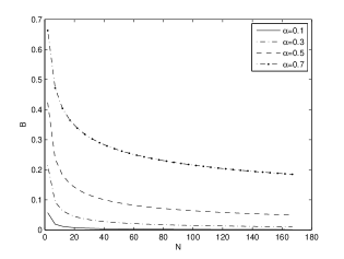
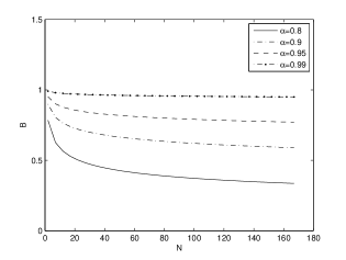
Figure 5.1: $B(\alpha,N)$ for different values of $\alpha$ and $N$.

Remark 23.

Similar computations give rise to an expansion formula for ${{}_{t}D_{b}^{\alpha}}$, the right Riemann–Liouville fractional derivative:

$${{}_{t}D_{b}^{\alpha}}x(t)\approx A(b-t)^{-\alpha}x(t)-B(b-t)^{1-\alpha}\dot{x}(t)-\sum_{p=2}^{N}C(\alpha,p)(b-t)^{1-p-\alpha}W_{p}(t),$$ (5.14)

where

$$W_{p}(t)=(1-p)\int_{t}^{b}(b-\tau)^{p-2}x(\tau)d\tau.$$

The coefficients $A=A(\alpha,N)$ and $B=B(\alpha,N)$ are the same as (5.11) and (5.12), respectively, and $C(\alpha,p)$ is given by (20).

Remark 24.

As stated before, Caputo derivatives are closely related to those of Riemann–Liouville. For any function, $x(\cdot)$, and for $\alpha\in(0,1)$, if these two kind of fractional derivatives exist, then we have

$${{}_{a}^{C}D_{t}^{\alpha}}x(t)={{}_{a}D_{t}^{\alpha}}x(t)-\frac{x(a)}{\Gamma(1-\alpha)}(t-a)^{-\alpha}$$

and

$${{}_{t}^{C}D_{b}^{\alpha}}x(t)={{}_{t}D_{b}^{\alpha}}x(t)-\frac{x(b)}{\Gamma(1-\alpha)}(b-t)^{-\alpha}.$$

Using these relations, we can easily construct approximation formulas for left and right Caputo fractional derivatives:

$${{}_{a}^{C}D_{t}^{\alpha}}x(t) \approx A(\alpha,N)(t-a)^{-\alpha}x(t)+B(\alpha,N)(t-a)^{1-\alpha}\dot{x}(t)$$

$$-\sum_{p=2}^{N}C(\alpha,p)(t-a)^{1-p-\alpha}V_{p}(t)-\frac{x(a)}{\Gamma(1-\alpha)}(t-a)^{-\alpha}.$$

Formula (5.7) consists of two parts: an infinite series and two terms including the first derivative and the function itself. It can be generalized to contain derivatives of higher-order.

Theorem 25.

Fix $n\in\mathbb{N}$ and let $x(\cdot)\in C^{n}[a,b]$. Then,

$${{}_{a}D_{t}^{\alpha}}x(t)=\frac{1}{\Gamma(1-\alpha)}(t-a)^{-\alpha}x(t)+\sum_{i=1}^{n-1}A(\alpha,i)(t-a)^{i-\alpha}x^{(i)}(t)\\ +\sum_{p=n}^{\infty}\left[\frac{-\Gamma(p-n+1+\alpha)}{\Gamma(-\alpha)\Gamma(1+\alpha)(p-n+1)!}(t-a)^{-\alpha}x(t)+B(\alpha,p)(t-a)^{n-1-p-\alpha}V_{p}(t)\right],$$ (5.15)

where

$$A(\alpha,i) = \frac{1}{\Gamma(i+1-\alpha)}\left[1+\sum_{p=n-i}^{\infty}\frac{\Gamma(p-n+1+\alpha)}{\Gamma(\alpha-i)(p-n+i+1)!}\right],\quad i=1,\ldots,n-1,$$

$$B(\alpha,p) = \frac{\Gamma(p-n+1+\alpha)}{\Gamma(-\alpha)\Gamma(1+\alpha)(p-n+1)!},$$

$$V_{p}(t) = (p-n+1)\int_{a}^{t}(\tau-a)^{p-n}x(\tau)d\tau.$$

Proof.

Successive integrating by parts in (5.6) gives

$${{}_{a}D_{t}^{\alpha}}x(t) = \frac{x(a)}{\Gamma(1-\alpha)}(t-a)^{-\alpha}+\frac{\dot{x}(a)}{\Gamma(2-\alpha)}(t-a)^{1-\alpha}+\cdots+\frac{x^{(n-1)}(a)}{\Gamma(n-\alpha)}(t-a)^{n-1-\alpha}$$

$$+\frac{1}{\Gamma(1-\alpha)}\int_{a}^{t}(t-\tau)^{n-1-\alpha}x^{(n)}(\tau)d\tau.$$

Using the binomial theorem, we expand the integral term as

$$\int_{a}^{t}(t-\tau)^{n-1-\alpha}x^{(n)}(\tau)d\tau=(t-a)^{n-1-\alpha}\sum_{p=0}^{\infty}\frac{\Gamma(p-n+1+\alpha)}{\Gamma(1-n+\alpha)p!(t-a)^{p}}\int_{a}^{t}(\tau-a)^{p}x^{(n)}(\tau)d\tau.$$

Splitting the sum into $p=0$ and $p=1\ldots\infty$, and integrating by parts the last integral, we get

$${{}_{a}D_{t}^{\alpha}}x(t) = \frac{(t-a)^{-\alpha}}{\Gamma(1-\alpha)}x(a)+\cdots+\frac{(t-a)^{n-2-\alpha}}{\Gamma(n-1-\alpha)}x^{(n-2)}(a)$$

$$+\frac{(t-a)^{n-1-\alpha}}{\Gamma(n-\alpha)}x^{(n-2)}(t)\left[1+\sum_{p=1}^{\infty}\frac{\Gamma(p-n+1+\alpha)}{\Gamma(-n+1+\alpha)p!}\right]$$

$$+\frac{(t-a)^{n-1-\alpha}}{\Gamma(n-1-\alpha)}\sum_{p=1}^{\infty}\frac{\Gamma(p-n+1+\alpha)}{\Gamma(-n+2+\alpha)(p-1)!(t-a)^{p}}\int_{a}^{t}(\tau-a)^{p-1}x^{(n-1)}(\tau)d\tau.$$

The rest of the proof follows a similar routine, i.e., by splitting the sum into two parts, the first term and the rest, and integrating by parts the last integral until $x(\cdot)$ appears in the integrand. ∎

Remark 26.

The series that appear in $A(\alpha,i)$ is convergent for all $i\in\{1,\ldots,n-1\}$. Fix an $i$ and observe that

$$\sum_{p=n-i}^{\infty}\frac{\Gamma(p-n+1+\alpha)}{\Gamma(\alpha-i)(p-n+i+1)!}=\sum_{p=1}^{\infty}\frac{\Gamma(p+\alpha-i)}{\Gamma(\alpha-i)p!}={{}_{1}F_{0}}(\alpha-i,1)-1,$$

where ${}_{1}F_{0}$ stands for a hypergeometric function [18]. Since $i>\alpha$, ${{}_{1}F_{0}}(\alpha-i,1)$ converges by Theorem 2.1.1 of [18].

In practice we only use finite sums and for $A(\alpha,i)$ we can easily compute the truncation error. Although this is a partial error, it gives a good intuition of why this approximation works well. Using the fact that ${{}_{1}F_{0}}(a,1)=0$ if $a<0$ (cf. Eq. (2.1.6) in [18]), we have

$$\begin{split}\frac{1}{\Gamma(i+1-\alpha)}&\sum_{p=N+1}^{\infty}\frac{\Gamma(p-n+1+\alpha)}{\Gamma(\alpha-i)(p-n+i+1)!}\\ &=\frac{1}{\Gamma(i+1-\alpha)}\left({{}_{1}F_{0}}(\alpha-i,1)-\sum_{p=0}^{N-n+i+1}\frac{\Gamma(p+\alpha-i)}{\Gamma(\alpha-i)p!}\right)\\ &=\frac{-1}{\Gamma(i+1-\alpha)}\sum_{p=0}^{N-n+i+1}\frac{\Gamma(p+\alpha-i)}{\Gamma(\alpha-i)p!}.\end{split}$$ (5.16)

In Table 5.2 we give some values for this error, with $\alpha=0.5$ and different values for $i$ and $N-n$.

	0	5	10	15	20
1	-0.4231	-0.2364	-0.1819	-0.1533	-0.1350
2	0.04702	0.009849	0.004663	0.002838	0.001956
3	-0.007052	-0.0006566	-0.0001999	-0.00008963	-0.00004890
4	0.001007	0.00004690	0.000009517	0.000003201	0.000001397

Table 5.2: The truncation error (5.16) of $A(\alpha,i)$ for $\alpha=0.5$, that is, $A(\alpha,i)-A(\alpha,i,N)$ with $A(\alpha,i,N)$ given by (5.18).

Remark 27.

Using Euler’s reflection formula, one can define $B(\alpha,p)$ of Theorem 25 as

$$B(\alpha,p)=\frac{-\sin(\pi\alpha)\Gamma(p-n+1+\alpha)}{\pi(p-n+1)!}.$$

For numerical purposes, only finite sums are taken to approximate fractional derivatives. Therefore, for a fixed $n\in\mathbb{N}$ and $N\geq n$, one has

$${{}_{a}D_{t}^{\alpha}}x(t)\approx\sum_{i=0}^{n-1}A(\alpha,i,N)(t-a)^{i-\alpha}x^{(i)}(t)+\sum_{p=n}^{N}B(\alpha,p)(t-a)^{n-1-p-\alpha}V_{p}(t),$$ (5.17)

where

$$A(\alpha,i,N)=\frac{1}{\Gamma(i+1-\alpha)}\left[1+\sum_{p=2}^{N}\frac{\Gamma(p-n+1+\alpha)}{\Gamma(\alpha-i)(p-n+i+1)!}\right],\quad i=0,\ldots,n-1,$$ (5.18)

$$B(\alpha,p) = \frac{\Gamma(p-n+1+\alpha)}{\Gamma(-\alpha)\Gamma(1+\alpha)(p-n+1)!},$$

$$V_{p}(t) = (p-n+1)\int_{a}^{t}(\tau-a)^{p-n}x(\tau)d\tau.$$

Similarly, we can deduce an expansion formula for the right fractional derivative.

Theorem 28.

Fix $n\in\mathbb{N}$ and $x(\cdot)\in C^{n}[a,b]$. Then,

$${{}_{t}D_{b}^{\alpha}}x(t)=\frac{1}{\Gamma(1-\alpha)}(b-t)^{-\alpha}x(t)+\sum_{i=1}^{n-1}A(\alpha,i)(b-t)^{i-\alpha}x^{(i)}(t)\\ +\sum_{p=n}^{\infty}\left[\frac{-\Gamma(p-n+1+\alpha)}{\Gamma(-\alpha)\Gamma(1+\alpha)(p-n+1)!}(b-t)^{-\alpha}x(t)+B(\alpha,p)(b-t)^{n-1-\alpha-p}W_{p}(t)\right],$$

where

$$A(\alpha,i) = \frac{(-1)^{i}}{\Gamma(i+1-\alpha)}\left[1+\sum_{p=n-i}^{\infty}\frac{\Gamma(p-n+1+\alpha)}{\Gamma(-i+\alpha)(p-n+1+i)!}\right],\quad i=1,\ldots,n-1,$$

$$B(\alpha,p) = \frac{(-1)^{n}\Gamma(p-n+1+\alpha)}{\Gamma(-\alpha)\Gamma(1+\alpha)(p-n+1)!},$$

$$W_{p}(t) = (p-n+1)\int_{t}^{b}(b-\tau)^{p-n}x(\tau)d\tau.$$

Proof.

Analogous to the proof of Theorem 25. ∎

5.1.3 Numerical evaluation of fractional derivatives

In [93] a numerical method to evaluate fractional derivatives is given based on the Grünwald–Letnikov definition of fractional derivatives. It uses the fact that for a large class of functions, the Riemann–Liouville and the Grünwald–Letnikov definitions are equivalent. We claim that the approximations discussed so far provide a good tool to compute numerically the fractional derivatives of given functions. For functions whose higher-order derivatives are easily available, we can freely choose between approximations (5.4) or (5.10). But in the case that difficulties arise in computing higher-order derivatives, we choose the approximation (5.10) that needs only the values of the first derivative and function itself. Even if the first derivative is not easily computable, we can use the approximation given by (5.13) with large values for $N$ and $\alpha$ not so close to one. As an example, we compute ${{}_{a}D_{t}^{\alpha}}x(t)$, with $\alpha=\frac{1}{2}$, for $x(t)=t^{4}$ and $x(t)=e^{2t}$. The exact formulas of the derivatives are derived from

$${{}_{0}D_{t}^{0.5}}(t^{n})=\frac{\Gamma(n+1)}{\Gamma(n+1-0.5)}t^{n-0.5}\quad\text{and}\quad{{}_{0}D_{t}^{0.5}}(e^{\lambda t})=t^{-0.5}E_{1,1-0.5}(\lambda t),$$

where $E_{\alpha,\beta}$ is the two parameter Mittag–Leffler function [93]. Figure 5.2 shows the results using approximation (5.4) with error $E$ computed by (3). As we can see, the third approximations are reasonably accurate for both cases. Indeed, for $x(t)=t^{4}$, the approximation with $N=4$ coincides with the exact solution because the derivatives of order five and more vanish.

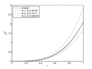
(a) ${{}_{0}D_{t}^{0.5}}(t^{4})$

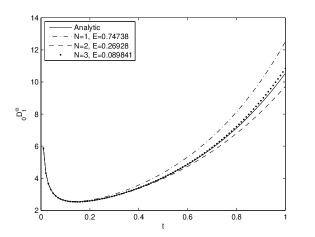
(b) ${{}_{0}D_{t}^{0.5}}(e^{2t})$

Figure 5.2: Analytic (solid line) versus numerical approximation (5.4).

The same computations are carried out using approximation (5.10). In this case, given a function $x(\cdot)$, we can compute $V_{p}$ by definition or integrate the system (5.9) analytically or by any numerical integrator. As it is clear from Figure 5.3, one can get better results by using larger values of $N$.

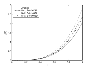
(a) ${{}_{0}D_{t}^{0.5}}(t^{4})$

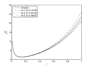
(b) ${{}_{0}D_{t}^{0.5}}(e^{2t})$

Figure 5.3: Analytic (solid line) versus numerical approximation (5.10).

Comparing Figures 5.2 and 5.3, we find out that the approximation (5.4) shows a faster convergence. Observe that both functions are analytic and it is easy to compute higher-order derivatives. The approximation (5.4) fails for non-analytic functions as stated in [23].

Remark 29.

A closer look to (5.4) and (5.10) reveals that in both cases the approximations are not computable at $a$ and $b$ for the left and right fractional derivatives, respectively. At these points we assume that it is possible to extend them continuously to the closed interval $[a,b]$.

In what follows, we show that by omitting the first derivative from the expansion, as done in [23], one may loose a considerable accuracy in computation. Once again, we compute the fractional derivatives of $x(t)=t^{4}$ and $x(t)=e^{2t}$, but this time we use the approximation given by (5.13). Figure 5.4 summarizes the results. The expansion up to the first derivative gives a more realistic approximation using quite small $N$, $3$ in this case.

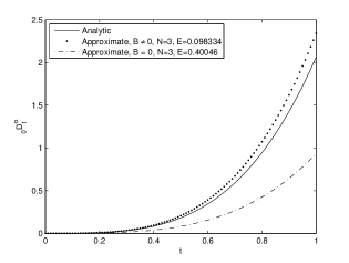
(a) ${{}_{0}D_{t}^{0.5}}(t^{4})$

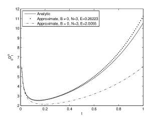
(b) ${{}_{0}D_{t}^{0.5}}(e^{2t})$

Figure 5.4: Comparison of approximation (5.10) proposed here and approximation (5.13) of [23].

To show how the appearance of higher-order derivatives in generalization (5.15) gives better results, we evaluate fractional derivatives of $x(t)=t^{4}$ and $x(t)=e^{2t}$ for different values of $n$. We consider $n=1,2,3$, $N=6$ for $x(t)=t^{4}$ (Figure 5.5(a)) and $N=4$ for $x(t)=e^{2t}$ (Figure 5.5(b)).

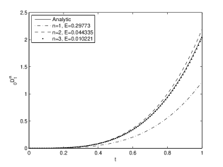
(a) ${{}_{0}D_{t}^{0.5}}(t^{4})$

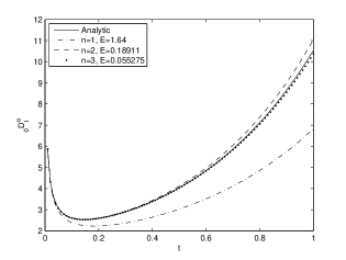
(b) ${{}_{0}D_{t}^{0.5}}(e^{2t})$

Figure 5.5: Analytic (solid line) versus numerical approximation (5.15).

5.1.4 Fractional derivatives of tabular data

In many situations, the function itself is not accessible in a closed form, but as a tabular data for discrete values of the independent variable. Thus, we cannot use the definition to compute the fractional derivative directly. Approximation (5.10) that uses the function and its first derivative to evaluate the fractional derivative, seems to be a good candidate in those cases. Suppose that we know the values of $x(t_{i})$ on $n+1$ distinct points in a given interval $[a,b]$, i.e., for $t_{i}$, $i=0,1,\ldots,n$, with $t_{0}=a$ and $t_{n}=b$. According to formula (5.10), the value of the fractional derivative of $x(\cdot)$ at each point $t_{i}$ is given approximately by

$${{}_{a}D_{t_{i}}^{\alpha}}x(t_{i})\approx A(\alpha,N)(t_{i}-a)^{-\alpha}x(t_{i})+B(\alpha,N)(t_{i}-a)^{1-\alpha}\dot{x}(t_{i})-\sum_{p=2}^{N}C(p,\alpha)(t_{i}-a)^{1-p-\alpha}V_{p}(t_{i}).$$

The values of $x(t_{i})$, $i=0,1,\ldots,n$, are given. A good approximation for $\dot{x}(t_{i})$ can be obtained using the forward, centered, or backward difference approximation of the first-order derivative [114]. For $V_{p}(t_{i})$ one can either use the definition and compute the integral numerically, i.e., $V_{p}(t_{i})=\int_{a}^{t_{i}}(1-p)(\tau-a)^{p-2}x(\tau)d\tau$, or it is possible to solve (5.9) as an initial value problem. All required computations are straightforward and only need to be implemented with the desired accuracy. The only thing to take care is the way of choosing a good order, $N$, in the formula (5.10). Because no value of $N$, guaranteeing the error to be smaller than a certain preassigned number, is known a priori, we start with some prescribed value for $N$ and increase it step by step. In each step we compare, using an appropriate norm, the result with the one of previous step. For instance, one can use the Euclidean norm $\|({{}_{a}D_{t}^{\alpha}})^{new}-({{}_{a}D_{t}^{\alpha}})^{old}\|_{2}$ and terminate the procedure when it’s value is smaller than a predefined $\epsilon$. For illustrative purposes, we compute the fractional derivatives of order $\alpha=0.5$ for tabular data extracted from $x(t)=t^{4}$ and $x(t)=e^{2t}$. The results are given in Figure 5.6.

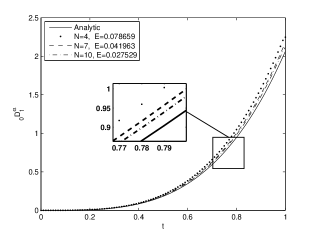
(a) ${{}_{0}D_{t}^{0.5}}(t^{4})$

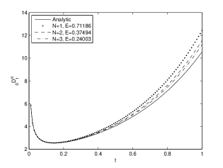
(b) ${{}_{0}D_{t}^{0.5}}(e^{2t})$

Figure 5.6: Fractional derivatives of tabular data.

5.1.5 Applications to fractional differential equations

The classical theory of ordinary differential equations is a well developed field with many tools available for numerical purposes. Using the approximations (5.4) and (5.10), one can transform a fractional ordinary differential equation into a classical ODE.

We should mention here that, using (5.4), derivatives of higher-order appear in the resulting ODE, while we only have a limited number of initial or boundary conditions available. In this case the value of $N$, the order of approximation, should be equal to the number of given conditions. If we choose a larger $N$, we will encounter lack of initial or boundary conditions. This problem is not present in the case in which we use the approximation (5.10), because the initial values for the auxiliary variables $V_{p}$, $p=2,3,\ldots$, are known and we don’t need any extra information.

Consider, as an example, the following initial value problem:

$$\left\{\begin{array}[]{l}{{}_{0}D_{t}^{0.5}}x(t)+x(t)=t^{2}+\frac{2}{\Gamma(2.5)}t^{\frac{3}{2}},\\ x(0)=0.\end{array}\right.$$ (5.19)

We know that ${{}_{0}D_{t}^{0.5}}(t^{2})=\frac{2}{\Gamma(2.5)}t^{\frac{3}{2}}$. Therefore, the analytic solution for system (5.19) is $x(t)=t^{2}$. Because only one initial condition is available, we can only expand the fractional derivative up to the first derivative in (5.4). One has

$$\left\{\begin{array}[]{l}1.5642~{}t^{-0.5}x(t)+0.5642~{}t^{0.5}\dot{x}(t)=t^{2}+1.5045~{}t^{1.5},\\ x(0)=0.\end{array}\right.$$ (5.20)

This is a classical initial value problem and can be easily treated numerically. The solution is drawn in Figure 5.7(a). As expected, the result is not satisfactory. Let us now use the approximation given by (5.10). The system in (5.19) becomes

$$\left\{\begin{array}[]{l}A(N)t^{-0.5}x(t)+B(N)t^{0.5}\dot{x}(t)-\sum_{p=2}^{N}C(p)t^{0.5-p}V_{p}+x(t)=t^{2}+\frac{2}{\Gamma(2.5)}t^{1.5},\\ \dot{V}_{p}(t)=(1-p)(t-a)^{p-2}x(t),\quad p=2,3,\ldots,N,\\ x(0)=0,\\ V_{p}(0)=0,\quad p=2,3,\ldots,N.\end{array}\right.$$ (5.21)

We solve this initial value problem for $N=7$. The MATLAB^® ode45 built-in function is used to integrate system (5.21). The solution is given in Figure 5.7(b) and shows a better approximation when compared with (5.20).

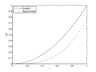
(a) Exact versus Approximation (5.4).

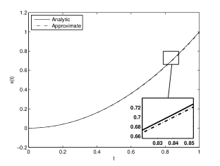
(b) Exact versus Approximation (5.10).

Figure 5.7: Two approximations applied to fractional differential equation (5.19).

Remark 30.

To show the difference caused by the appearance of the first derivative in formula (5.10), we solve the initial value problem (5.19) with $B(\alpha,N)=0$. Since the original fractional differential equation does not depend on integer-order derivatives of function $x(\cdot)$, i.e., it has the form

$${{}_{a}D_{t}^{\alpha}}x(t)+f(x,t)=0,$$

by (5.13) the dependence to derivatives of $x(\cdot)$ vanishes. In this case one needs to apply the operator ${}_{a}D_{t}^{1-\alpha}$ to the above equation and obtain

$$\dot{x}(t)+_{a}D_{t}^{1-\alpha}[f(x,t)]=0.$$

Nevertheless, we can use (5.10) directly without any trouble. Figure 5.8 shows that at least for a moderate accurate method, like the MATLAB^® routine ode45, taking $B(\alpha,N)\neq 0$ into account gives a better approximation.

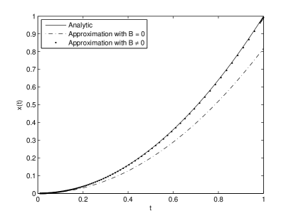
Figure 5.8: Comparison of our approach to that of [23].

5.2 Hadamard derivatives

For Hadamard derivatives, the expansions can be obtained in a quite similar way and are introduced next [97].

5.2.1 Approximation by a sum of integer-order derivatives

Assume that a function $x(\cdot)$ admits derivatives of any order, then expansion formulas for the Hadamard fractional integrals and derivatives of $x$, in terms of its integer-order derivatives, are given in [35, Theorem 17]:

$${{}_{0}\mathcal{I}_{t}^{\alpha}}x(t)=\sum_{k=0}^{\infty}S(-\alpha,k)t^{k}x^{(k)}(t)$$

and

$${{}_{0}\mathcal{D}_{t}^{\alpha}}x(t)=\sum_{k=0}^{\infty}S(\alpha,k)t^{k}x^{(k)}(t),$$

where

$$S(\alpha,k)=\frac{1}{k!}\sum_{j=1}^{k}(-1)^{k-j}{k\choose j}j^{\alpha}$$

is the Stirling function.

As approximations we truncate infinite sums at an appropriate order $N$ and get the following forms:

$${{}_{0}\mathcal{I}_{t}^{\alpha}}x(t)=\sum_{k=0}^{N}S(-\alpha,k)t^{k}x^{(k)}(t)$$

and

$${{}_{0}\mathcal{D}_{t}^{\alpha}}x(t)=\sum_{k=0}^{N}S(\alpha,k)t^{k}x^{(k)}(t).$$

5.2.2 Approximation using moments of a function

The same idea of expanding Riemann–Liouville derivatives, with slightly different techniques, is used to derive expansion formulas for left and right Hadamard derivatives. The following lemma is the basis for such new relations.

Lemma 31.

Let $\alpha\in(0,1)$ and $x(\cdot)$ be an absolutely continuous function on $[a,b]$. Then the Hadamard fractional derivatives may be expressed by

$${{}_{a}\mathcal{D}_{t}^{\alpha}}x(t)=\frac{x(a)}{\Gamma(1-\alpha)}\left(\ln\frac{t}{a}\right)^{-\alpha}+\frac{1}{\Gamma(1-\alpha)}\int_{a}^{t}\left(\ln\frac{t}{\tau}\right)^{-\alpha}\dot{x}(\tau)d\tau$$ (5.22)

and

$${{}_{t}\mathcal{D}_{b}^{\alpha}}x(t)=\frac{x(b)}{\Gamma(1-\alpha)}\left(\ln\frac{b}{t}\right)^{-\alpha}-\frac{1}{\Gamma(1-\alpha)}\int_{t}^{b}\left(\ln\frac{\tau}{t}\right)^{-\alpha}\dot{x}(\tau)d\tau.$$ (5.23)

A proof of this lemma for an arbitrary $\alpha>0$ can be found in [65, Theorem 3.2].

Applying similar techniques as presented in Theorem 25 to the formulas (5.22) and (5.23) gives the following theorem.

Theorem 32.

Let $n\in\mathbb{N}$, $0<a<b$ and $x:[a,b]\to\mathbb{R}$ be a function of class $C^{n+1}$. Then

$${{}_{a}\mathcal{D}_{t}^{\alpha}}x(t)\approx\sum_{i=0}^{n}A_{i}(\alpha,N)\left(\ln\frac{t}{a}\right)^{i-\alpha}x_{i,0}(t)+\sum_{p=n+1}^{N}B(\alpha,p)\left(\ln\frac{t}{a}\right)^{n-\alpha-p}V_{p}(t)$$

with

$$\begin{array}[]{rl}A_{i}(\alpha,N)&=\displaystyle\frac{1}{\Gamma(i+1-\alpha)}\left[1+\sum_{p=n-i+1}^{N}\frac{\Gamma(p+\alpha-n)}{\Gamma(\alpha-i)(p-n+i)!}\right],\quad i\in\{0,\ldots,n\},\\[12.0pt] B(\alpha,p)&=\displaystyle\frac{\Gamma(p+\alpha-n)}{\Gamma(-\alpha)\Gamma(1+\alpha)(p-n)!},\quad p\in\{n+1,\ldots\},\\[12.0pt] V_{p}(t)&=\displaystyle\int_{a}^{t}(p-n)\left(\ln\frac{\tau}{a}\right)^{p-n-1}\frac{x(\tau)}{\tau}d\tau,\quad p\in\{n+1,\ldots\}.\end{array}$$

Remark 33.

The right Hadamard fractional derivative can be expanded in the same way. This gives the following approximation:

$${{}_{t}\mathcal{D}_{b}^{\alpha}}x(t) \approx A(\alpha,N)\left(\ln\frac{b}{t}\right)^{-\alpha}x(t)-B(\alpha,N)\left(\ln\frac{b}{t}\right)^{1-\alpha}t\dot{x}(t)$$

$$\quad-\sum_{p=2}^{N}C(\alpha,p)\left(\ln\frac{b}{t}\right)^{1-\alpha-p}W_{p}(t),$$

with

$$W_{p}(t)=(1-p)\int_{t}^{b}\left(\ln\frac{b}{\tau}\right)^{p-2}\frac{x(\tau)}{\tau}d\tau.$$

Remark 34.

In the particular case $n=1$, one obtains from Theorem 32 that

$${{}_{a}\mathcal{D}_{t}^{\alpha}}x(t) \approx A(\alpha,N)\left(\ln\frac{t}{a}\right)^{-\alpha}x(t)+B(\alpha,N)\left(\ln\frac{t}{a}\right)^{1-\alpha}t\dot{x}(t)$$ (5.24)

$$\quad+\sum_{p=2}^{N}C(\alpha,p)\left(\ln\frac{t}{a}\right)^{1-\alpha-p}V_{p}(t)$$

with

$$A(\alpha,N) = \frac{1}{\Gamma(1-\alpha)}\left(1+\sum_{p=2}^{N}\frac{\Gamma(p+\alpha-1)}{\Gamma(\alpha)(p-1)!}\right),$$

$$B(\alpha,N) = \frac{1}{\Gamma(2-\alpha)}\left(1+\sum_{p=1}^{N}\frac{\Gamma(p+\alpha-1)}{\Gamma(\alpha-1)p!}\right).$$

5.2.3 Examples

In this section we apply (5.24) to compute fractional derivatives, of order $\alpha=0.5$, for $x(t)=\ln(t)$ and $x(t)=t^{4}$. The exact Hadamard fractional derivative is available for $x(t)=\ln(t)$ and we have

$${{}_{1}\mathcal{D}_{t}^{0.5}}(\ln(t))=\frac{\sqrt{\ln t}}{\Gamma(1.5)}.$$

For $x(t)=t^{4}$ only an approximation of Hadamard fractional derivative is found in the literature:

$${{}_{1}\mathcal{D}_{t}^{0.5}}t^{4}\approx\frac{1}{\Gamma(0.5)\sqrt{\ln t}}+\frac{0.5908179503}{\Gamma(0.5)}4t^{4}\mbox{erf}(3\sqrt{\ln t}),$$

where $\mbox{erf}(\cdot)$ in the so-called Gauss error function,

$$\mbox{erf}(t)=\frac{1}{\sqrt{\pi}}\int_{0}^{t}e^{-\tau^{2}}\,d\tau.$$

The results of applying (5.24) to evaluate fractional derivatives are depicted in Figure 5.9.

(a) ${{}_{1}\mathcal{D}_{t}^{0.5}}(\ln t)$

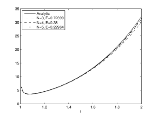
(b) ${{}_{1}\mathcal{D}_{t}^{0.5}}(t^{4})$

Figure 5.9: Analytic versus numerical approximation (5.24).

As another example, we consider the following fractional differential equation involving a Hadamard fractional derivative:

$$\left\{\begin{array}[]{l}\displaystyle{{}_{1}\mathcal{D}_{t}^{0.5}}x(t)+x(t)=\frac{\sqrt{x(t)}}{\Gamma(1.5)}+\ln t\\ x(1)=0.\end{array}\right.$$ (5.25)

Obviously, $x(t)=\ln t$ is a solution for (5.25). Since we have only one initial condition, we replace the operator ${{}_{1}\mathcal{D}_{t}^{0.5}}(\cdot)$ by the expansion with $n=1$ and thus obtaining

$$\left\{\begin{array}[]{l}\displaystyle\left[1+A_{0}(\ln t)^{-0.5}\right]x(t)+A_{1}(\ln t)^{0.5}t\dot{x}(t)+\sum_{p=2}^{N}B(0.5,p)(\ln t)^{0.5-p}V_{p}(t)=\frac{\sqrt{x(t)}}{\Gamma(1.5)}+\ln t,\\ \displaystyle\dot{V_{p}}(t)=(p-1)(\ln t)^{p-2}\frac{x(t)}{t},\quad p=2,3,\ldots,N,\\ x(1)=0,\\ V_{p}(1)=0,\quad p=2,3,\ldots,N.\end{array}\right.$$ (5.26)

In Figure 5.10 we compare the analytical solution of problem (5.25) with the numerical result for $N=2$ in (5.26).

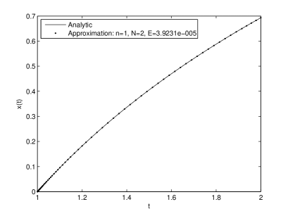
Figure 5.10: Analytic versus numerical approximation for problem (5.25) with one initial condition.

5.3 Error analysis

When we approximate an infinite series by a finite sum, the choice of the order of approximation is a key question. Having an estimate knowledge of truncation errors, one can choose properly up to which order the approximations should be made to suit the accuracy requirements. In this section we study the errors of the approximations presented so far.

Separation of an error term in (5.3) ends in

$${{}_{a}D_{t}^{\alpha}}x(t) = \frac{1}{\Gamma(1-\alpha)}\frac{d}{dt}\int_{a}^{t}\left((t-\tau)^{-\alpha}\sum_{k=0}^{N}\frac{(-1)^{k}x^{(k)}(t)}{k!}(t-\tau)^{k}\right)d\tau$$ (5.27)

$$+\frac{1}{\Gamma(1-\alpha)}\frac{d}{dt}\int_{a}^{t}\left((t-\tau)^{-\alpha}\sum_{k=N+1}^{\infty}\frac{(-1)^{k}x^{(k)}(t)}{k!}(t-\tau)^{k}\right)d\tau.$$

The first term in (5.27) gives (5.4) directly and the second term is the error caused by truncation. The next step is to give a local upper bound for this error, $E_{tr}(t)$.

The series

$$\sum_{k=N+1}^{\infty}\frac{(-1)^{k}x^{(k)}(t)}{k!}(t-\tau)^{k},\quad\tau\in(a,t),\quad t\in(a,b),$$

is the remainder of the Taylor expansion of $x(\tau)$ and thus bounded by $\left|\frac{M}{(N+1)!}(t-\tau)^{N+1}\right|$ in which

$$M=\displaystyle\max_{\tau\in[a,t]}|x^{(N+1)}(\tau)|.$$

Then,

$$E_{tr}(t)\leq\left|\frac{M}{\Gamma(1-\alpha)(N+1)!}\frac{d}{dt}\int_{a}^{t}(t-\tau)^{N+1-\alpha}d\tau\right|=\frac{M}{\Gamma(1-\alpha)(N+1)!}(t-a)^{N+1-\alpha}.$$

In order to estimate a truncation error for approximation (5.10), the expansion procedure is carried out with separation of $N$ terms in binomial expansion as

$$\left(1-\frac{\tau-a}{t-a}\right)^{1-\alpha} = \sum_{p=0}^{\infty}\frac{\Gamma(p-1+\alpha)}{\Gamma(\alpha-1)p!}\left(\frac{\tau-a}{t-a}\right)^{p}$$ (5.28)

$$= \sum_{p=0}^{N}\frac{\Gamma(p-1+\alpha)}{\Gamma(\alpha-1)p!}\left(\frac{\tau-a}{t-a}\right)^{p}+R_{N}(\tau),$$

where

$$R_{N}(\tau)=\sum_{p=N+1}^{\infty}\frac{\Gamma(p-1+\alpha)}{\Gamma(\alpha-1)p!}\left(\frac{\tau-a}{t-a}\right)^{p}.$$

Integration by parts on the right-hand-side of (5.6) gives

$${{}_{a}D_{t}^{\alpha}}x(t)=\frac{x(a)}{\Gamma(1-\alpha)}(t-a)^{-\alpha}+\frac{\dot{x}(a)}{\Gamma(2-\alpha)}(t-a)^{1-\alpha}+\frac{1}{\Gamma(2-\alpha)}\int_{a}^{t}(t-\tau)^{1-\alpha}\ddot{x}(\tau)d\tau.$$ (5.29)

Substituting (5.28) into (5.29), we get

$${{}_{a}D_{t}^{\alpha}}x(t) = \frac{x(a)}{\Gamma(1-\alpha)}(t-a)^{-\alpha}+\frac{\dot{x}(a)}{\Gamma(2-\alpha)}(t-a)^{1-\alpha}$$

$$+\frac{(t-a)^{1-\alpha}}{\Gamma(2-\alpha)}\int_{a}^{t}\left(\sum_{p=0}^{N}\frac{\Gamma(p-1+\alpha)}{\Gamma(\alpha-1)p!}\left(\frac{\tau-a}{t-a}\right)^{p}+R_{N}(\tau)\right)\ddot{x}(\tau)d\tau$$

$$= \frac{x(a)}{\Gamma(1-\alpha)}(t-a)^{-\alpha}+\frac{\dot{x}(a)}{\Gamma(2-\alpha)}(t-a)^{1-\alpha}$$

$$+\frac{(t-a)^{1-\alpha}}{\Gamma(2-\alpha)}\int_{a}^{t}\left(\sum_{p=0}^{N}\frac{\Gamma(p-1+\alpha)}{\Gamma(\alpha-1)p!}\left(\frac{\tau-a}{t-a}\right)^{p}\right)\ddot{x}(\tau)d\tau$$

$$+\frac{(t-a)^{1-\alpha}}{\Gamma(2-\alpha)}\int_{a}^{t}R_{N}(\tau)\ddot{x}(\tau)d\tau.$$

At this point, we apply the techniques of [23] to the first three terms with finite sums. Then, we receive (5.10) with an extra term of truncation error:

$$E_{tr}(t)=\frac{(t-a)^{1-\alpha}}{\Gamma(2-\alpha)}\int_{a}^{t}R_{N}(\tau)\ddot{x}(\tau)d\tau.$$

Since $0\leq\frac{\tau-a}{t-a}\leq 1$ for $\tau\in[a,t]$, one has

$$|R_{N}(\tau)| \leq \sum_{p=N+1}^{\infty}\left|\frac{\Gamma(p-1+\alpha)}{\Gamma(\alpha-1)p!}\right|=\sum_{p=N+1}^{\infty}\left|\binom{1-\alpha}{p}\right|\leq\sum_{p=N+1}^{\infty}\frac{\mathrm{e}^{(1-\alpha)^{2}+1-\alpha}}{p^{2-\alpha}}$$

$$\leq \int_{p=N}^{\infty}\frac{\mathrm{e}^{(1-\alpha)^{2}+1-\alpha}}{p^{2-\alpha}}dp=\frac{\mathrm{e}^{(1-\alpha)^{2}+1-\alpha}}{(1-\alpha)N^{1-\alpha}}.$$

Finally, assuming $L_{n}=\displaystyle\max_{\tau\in[a,t]}\left|x^{(n)}(\tau)\right|$, we conclude that

$$|E_{tr}(t)|\leq L_{2}\frac{\mathrm{e}^{(1-\alpha)^{2}+1-\alpha}}{\Gamma(2-\alpha)(1-\alpha)N^{1-\alpha}}(t-a)^{2-\alpha}.$$

In the general case, the error is given by the following result.

Theorem 35.

If we approximate the left Riemann–Liouville fractional derivative by the finite sum (5.17), then the error $E_{tr}(\cdot)$ is bounded by

$$|E_{tr}(t)|\leq L_{n}\frac{\mathrm{e}^{(n-1-\alpha)^{2}+n-1-\alpha}}{\Gamma(n-\alpha)(n-1-\alpha)N^{n-1-\alpha}}(t-a)^{n-\alpha}.$$ (5.30)

From (5.30) we see that if the test function grows very fast or the point $t$ is far from $a$, then the value of $N$ should also increase in order to have a good approximation. Clearly, if we increase the value of $n$, then we need also to increase the value of $N$ to control the error.

Remark 36.

Following similar techniques, one can extract an error bound for the approximations of Hadamard derivatives. When we consider finite sums in (5.24), the error is bounded by

$$\left|E_{tr}(t)\right|\leq L(t)\frac{e^{(1-\alpha)^{2}+1-\alpha}}{\Gamma(2-\alpha)(1-\alpha)N^{1-\alpha}}\left(\ln\frac{t}{a}\right)^{1-\alpha}(t-a),$$

where

$$L(t)=\max_{\tau\in[a,t]}|\dot{x}(\tau)+\tau\ddot{x}(\tau)|.$$

For the general case, the expansion up to the derivative of order $n$, the error is bounded by

$$\left|E_{tr}(t)\right|\leq L_{n}(t)\frac{e^{(n-\alpha)^{2}+n-\alpha}}{\Gamma(n+1-\alpha)(n-\alpha)N^{n-\alpha}}\left(\ln\frac{t}{a}\right)^{n-\alpha}(t-a),$$

where

$$L_{n}(t)=\max_{\tau\in[a,t]}|x_{n,1}(\tau)|.$$

Chapter 6 Approximating fractional integrals

We obtain a new decomposition of the Riemann–Liouville operators of fractional integration as a series involving derivatives (of integer order). The new formulas are valid for functions of class $C^{n}$, $n\in\mathbb{N}$, and allow us to develop suitable numerical approximations with known estimations for the error. The usefulness of the obtained results, in solving fractional integral equations, is illustrated [95].

6.1 Riemann–Liouville fractional integral

6.1.1 Approximation by a sum of integer-order derivatives

For analytical functions, we can rewrite the left Riemann–Liouville fractional integral as a series involving integer-order derivatives only. If $x$ is analytic in $[a,b]$, then

$${{}_{a}I_{t}^{\alpha}}x(t)=\frac{1}{\Gamma(\alpha)}\sum_{k=0}^{\infty}\frac{(-1)^{k}(t-a)^{k+\alpha}}{(k+\alpha)k!}x^{(k)}(t)$$ (6.1)

for all $t\in[a,b]$ (cf. Eq. (3.44) in [83]). From the numerical point of view, one considers finite sums and the following approximation:

$${{}_{a}I_{t}^{\alpha}}x(t)\approx\frac{1}{\Gamma(\alpha)}\sum_{k=0}^{N}\frac{(-1)^{k}(t-a)^{k+\alpha}}{(k+\alpha)k!}x^{(k)}(t).$$ (6.2)

One problem with formula (6.1) is that in order to have a “good” approximation we need to take a large value for $n$. In applications, this approach may not be suitable. Here we present a new decomposition formula for functions of class $C^{n}$. The advantage is that even for $n=1$, we can achieve an appropriate accuracy.

6.1.2 Approximation using moments of a function

Before we give the result in its full extension, we explain the method for $n=3$. To that purpose, let $x\in C^{3}[a,b]$. Using integration by parts three times, we deduce that

$${{}_{a}I_{t}^{\alpha}}x(t) = \frac{x(a)}{\Gamma(\alpha+1)}(t-a)^{\alpha}+\frac{\dot{x}(a)}{\Gamma(\alpha+2)}(t-a)^{\alpha+1}+\frac{\ddot{x}(a)}{\Gamma(\alpha+3)}(t-a)^{\alpha+2}$$

$$+\frac{1}{\Gamma(\alpha+3)}\int_{a}^{t}(t-\tau)^{\alpha+2}x^{(3)}(\tau)d\tau.$$

By the binomial formula, we can rewrite the fractional integral as

$${{}_{a}I_{t}^{\alpha}}x(t) = \frac{x(a)}{\Gamma(\alpha+1)}(t-a)^{\alpha}+\frac{\dot{x}(a)}{\Gamma(\alpha+2)}(t-a)^{\alpha+1}+\frac{\ddot{x}(a)}{\Gamma(\alpha+3)}(t-a)^{\alpha+2}$$

$$+\frac{(t-a)^{\alpha+2}}{\Gamma(\alpha+3)}\sum_{p=0}^{\infty}\frac{\Gamma(p-\alpha-2)}{\Gamma(-\alpha-2)p!(t-a)^{p}}\int_{a}^{t}(\tau-a)^{p}x^{(3)}(\tau)d\tau.$$

The rest of the procedure follows the same pattern: decompose the sum into a first term plus the others, and integrate by parts. Then assuming

$$\begin{array}[]{ll}A_{0}(\alpha)&=\displaystyle\frac{1}{\Gamma(\alpha+1)}\left[1+\sum_{p=3}^{\infty}\frac{\Gamma(p-\alpha-2)}{\Gamma(-\alpha)(p-2)!}\right],\\ A_{1}(\alpha)&=\displaystyle\frac{1}{\Gamma(\alpha+2)}\left[1+\sum_{p=2}^{\infty}\frac{\Gamma(p-\alpha-2)}{\Gamma(-\alpha-1)(p-1)!}\right],\\ A_{2}(\alpha)&=\displaystyle\frac{1}{\Gamma(\alpha+3)}\left[1+\sum_{p=1}^{\infty}\frac{\Gamma(p-\alpha-2)}{\Gamma(-\alpha-2)p!}\right],\\ \end{array}$$

we obtain

$$\begin{split}{{}_{a}I_{t}^{\alpha}}x(t)&=\frac{x(a)}{\Gamma(\alpha+1)}(t-a)^{\alpha}+\frac{\dot{x}(a)}{\Gamma(\alpha+2)}(t-a)^{\alpha+1}+A_{2}(\alpha)(t-a)^{\alpha+2}\ddot{x}(t)\\ &\quad+\frac{(t-a)^{\alpha+2}}{\Gamma(\alpha+2)}\sum_{p=1}^{\infty}\frac{\Gamma(p-\alpha-2)}{\Gamma(-\alpha-1)(p-1)!(t-a)^{p}}\int_{a}^{t}(\tau-a)^{p-1}\ddot{x}(\tau)d\tau\\ &=\frac{x(a)}{\Gamma(\alpha+1)}(t-a)^{\alpha}+A_{1}(\alpha)(t-a)^{\alpha+1}\dot{x}(t)+A_{2}(\alpha)(t-a)^{\alpha+2}\ddot{x}(t)\\ &\quad+\frac{(t-a)^{\alpha+2}}{\Gamma(\alpha+1)}\sum_{p=2}^{\infty}\frac{\Gamma(p-\alpha-2)}{\Gamma(-\alpha)(p-2)!(t-a)^{p}}\int_{a}^{t}(\tau-a)^{p-2}\dot{x}(\tau)d\tau\\ &=A_{0}(\alpha)(t-a)^{\alpha}x(t)+A_{1}(\alpha)(t-a)^{\alpha+1}\dot{x}(t)+A_{2}(\alpha)(t-a)^{\alpha+2}\ddot{x}(t)\\ &\quad+\frac{(t-a)^{\alpha+2}}{\Gamma(\alpha)}\sum_{p=3}^{\infty}\frac{\Gamma(p-\alpha-2)}{\Gamma(-\alpha+1)(p-3)!(t-a)^{p}}\int_{a}^{t}(\tau-a)^{p-3}x(\tau)d\tau.\end{split}$$

Therefore, we can expand ${{}_{a}I_{t}^{\alpha}}x(t)$ as

$${{}_{a}I_{t}^{\alpha}}x(t)=A_{0}(\alpha)(t-a)^{\alpha}x(t)+A_{1}(\alpha)(t-a)^{\alpha+1}\dot{x}(t)+A_{2}(\alpha)(t-a)^{\alpha+2}\ddot{x}(t)\\ +\sum_{p=3}^{\infty}B(\alpha,p)(t-a)^{\alpha+2-p}V_{p}(t),$$ (6.3)

where

$$B(\alpha,p)=\frac{\Gamma(p-\alpha-2)}{\Gamma(\alpha)\Gamma(1-\alpha)(p-2)!},$$ (6.4)

and

$$V_{p}(t)=\int_{a}^{t}(p-2)(\tau-a)^{p-3}x(\tau)d\tau.$$ (6.5)

Remark 37.

Function $V_{p}$ given by (6.5) may be defined as the solution of the differential equation

$$\left\{\begin{array}[]{l}\dot{V}_{p}(t)=(p-2)(t-a)^{p-3}x(t)\\ V_{p}(a)=0,\end{array}\right.$$

for $p=3,4,\ldots$

Remark 38.

When $\alpha$ is not an integer, we may use Euler’s reflection formula (cf. [28])

$$\Gamma(\alpha)\Gamma(1-\alpha)=\frac{\pi}{\sin(\pi\alpha)},$$

to simplify expression $B(\alpha,p)$ in (6.4).

Following the same reasoning, we are able to deduce a general formula of decomposition for fractional integrals, depending on the order of smoothness of the test function.

Theorem 39.

Let $n\in\mathbb{N}$ and $x\in C^{n}[a,b]$. Then

$${{}_{a}I_{t}^{\alpha}}x(t)=\sum_{i=0}^{n-1}A_{i}(\alpha)(t-a)^{\alpha+i}x^{(i)}(t)+\sum_{p=n}^{\infty}B(\alpha,p)(t-a)^{\alpha+n-1-p}V_{p}(t),$$ (6.6)

where

$$\begin{array}[]{ll}A_{i}(\alpha)&=\displaystyle\frac{1}{\Gamma(\alpha+i+1)}\left[1+\sum_{p=n-i}^{\infty}\frac{\Gamma(p-\alpha-n+1)}{\Gamma(-\alpha-i)(p-n+1+i)!}\right],\quad i=0,\ldots,n-1,\\ B(\alpha,p)&=\displaystyle\frac{\Gamma(p-\alpha-n+1)}{\Gamma(\alpha)\Gamma(1-\alpha)(p-n+1)!},\end{array}$$ (6.7)

and

$$V_{p}(t)=\int_{a}^{t}(p-n+1)(\tau-a)^{p-n}x(\tau)d\tau,$$ (6.8)

$p=n,n+1,\ldots$

A remark about the convergence of the series in $A_{i}(\alpha)$, for $i\in\{0,\ldots,n-1\}$, is in order. Since

$$\begin{array}[]{ll}\displaystyle\sum_{p=n-i}^{\infty}\frac{\Gamma(p-\alpha-n+1)}{\Gamma(-\alpha-i)(p-n+1+i)!}&=\displaystyle\sum_{p=0}^{\infty}\frac{\Gamma(p-\alpha-i)}{\Gamma(-\alpha-i)p!}-1\\ &={{}_{1}F_{0}}(-\alpha-i,1),\\ \end{array}$$ (6.9)

where ${{}_{1}F_{0}}$ denotes the hypergeometric function, and because $\alpha+i>0$, we conclude that (6.9) converges absolutely (cf. Theorem 2.1.2 in [18]). In fact, we may use Eq. (2.1.6) in [18] to conclude that

$$\sum_{p=n-i}^{\infty}\frac{\Gamma(p-\alpha-n+1)}{\Gamma(-\alpha-i)(p-n+1+i)!}=-1.$$

Therefore, the first $n$ terms of our decomposition (6.6) vanish. However, because of numerical reasons, we do not follow this procedure here. Indeed, only finite sums of these coefficients are to be taken, and we obtain a better accuracy for the approximation taking them into account (see Figures 6.5(a) and 6.5(b)). More precisely, we consider finite sums up to order $N$, with $N\geq n$. Thus, our approximation will depend on two parameters: the order of the derivative $n\in\mathbb{N}$, and the number of terms taken in the sum, which is given by $N$. The left fractional integral is then approximated by

$${{}_{a}I_{t}^{\alpha}}x(t)\approx\sum_{i=0}^{n-1}A_{i}(\alpha,N)(t-a)^{\alpha+i}x^{(i)}(t)+\sum_{p=n}^{N}B(\alpha,p)(t-a)^{\alpha+n-1-p}V_{p}(t),$$ (6.10)

where

$$A_{i}(\alpha,N)=\frac{1}{\Gamma(\alpha+i+1)}\left[1+\sum_{p=n-i}^{N}\frac{\Gamma(p-\alpha-n+1)}{\Gamma(-\alpha-i)(p-n+1+i)!}\right],$$ (6.11)

and $B(\alpha,p)$ and $V_{p}(t)$ are given by (6.7) and (6.8), respectively.

To measure the truncation errors made by neglecting the remaining terms, observe that

$$\begin{split}\frac{1}{\Gamma(\alpha+i+1)}&\sum_{p=N+1}^{\infty}\frac{\Gamma(p-\alpha-n+1)}{\Gamma(-\alpha-i)(p-n+1+i)!}=\frac{1}{\Gamma(\alpha+i+1)}\sum_{p=N-n+2+i}^{\infty}\frac{\Gamma(p-\alpha-i)}{\Gamma(-\alpha-i)p!}\\ &=\frac{1}{\Gamma(\alpha+i+1)}\left[{{}_{2}F_{1}}(-\alpha-i,-,-,1)-\sum_{p=0}^{N-n+1+i}\frac{\Gamma(p-\alpha-i)}{\Gamma(-\alpha-i)p!}\right]\\ &=\frac{-1}{\Gamma(\alpha+i+1)}\sum_{p=0}^{N-n+i+1}\frac{\Gamma(p-\alpha-i)}{\Gamma(-\alpha-i)p!}.\end{split}$$ (6.12)

Similarly,

$$\frac{1}{\Gamma(\alpha)\Gamma(1-\alpha)}\sum_{p=N+1}^{\infty}\frac{\Gamma(p-\alpha-n+1)}{(p-n+1)!}=\frac{-1}{\Gamma(\alpha)\Gamma(1-\alpha)}\sum_{p=0}^{N-n+1}\frac{\Gamma(p-\alpha)}{p!}.$$ (6.13)

In Tables 6.1 and 6.2 we exemplify some values for (6.12) and (6.13), respectively, with $\alpha=0.5$ and for different values of $N$, $n$ and $i$. Observe that the errors only depend on the values of $N-n$ and $i$ for (6.12), and on the value of $N-n$ for (6.13).

	0	1	2	3	4
0	-0.5642	-0.4231	-0.3526	-0.3085	-0.2777
1	0.09403	0.04702	0.02938	0.02057	0.01543
2	-0.01881	-0.007052	-0.003526	-0.002057	-0.001322
3	0.003358	0.001007	0.0004198	0.0002099	0.0001181
4	-0.0005224	-0.0001306	-0.00004664	-0.00002041	-0.00001020
5	$7.12\times 10^{-5}$	$1.52\times 10^{-5}$	$4.77\times 10^{-6}$	$1.85\times 10^{-6}$	$8.34\times 10^{-7}$

Table 6.1: Values of error (6.12) for $\alpha=0.5$.

$N-n$	0	1	2	3	4
	0.5642	0.4231	0.3526	0.3085	0.2777

Table 6.2: Values of error (6.13) for $\alpha=0.5$.

Everything done so far is easily adapted to the right fractional integral. In fact, one has:

Theorem 40.

Let $n\in\mathbb{N}$ and $x\in C^{n}[a,b]$. Then

$${{}_{t}I_{b}^{\alpha}}x(t)=\sum_{i=0}^{n-1}A_{i}(\alpha)(b-t)^{\alpha+i}x^{(i)}(t)+\sum_{p=n}^{\infty}B(\alpha,p)(b-t)^{\alpha+n-1-p}W_{p}(t),$$

where

$$\begin{split}A_{i}(\alpha)&=\frac{(-1)^{i}}{\Gamma(\alpha+i+1)}\left[1+\sum_{p=n-i}^{\infty}\frac{\Gamma(p-\alpha-n+1)}{\Gamma(-\alpha-i)(p-n+1+i)!}\right],\\ B(\alpha,p)&=\frac{(-1)^{n}\Gamma(p-\alpha-n+1)}{\Gamma(\alpha)\Gamma(1-\alpha)(p-n+1)!},\\ W_{p}(t)&=\int_{t}^{b}(p-n+1)(b-\tau)^{p-n}x(\tau)d\tau.\end{split}$$

6.1.3 Numerical evaluation of fractional integrals

In this section we exemplify the proposed approximation procedure with some examples. In each step, we evaluate the accuracy of our method, i.e., the error when substituting ${{}_{a}I_{t}^{\alpha}}x$ by an approximation $\tilde{{{}_{a}I_{t}^{\alpha}}}x$. For that purpose, we take the distance given by

$$E=\sqrt{\int_{a}^{b}\left({{}_{a}I_{t}^{\alpha}}x(t)-\tilde{{{}_{a}I_{t}^{\alpha}}}x(t)\right)^{2}dt}.$$

Firstly, consider $x_{1}(t)=t^{3}$ and $x_{2}(t)=t^{10}$ with $t\in[0,1]$. Then

$${{}_{0}I_{t}^{0.5}}x_{1}(t)=\frac{\Gamma(4)}{\Gamma(4.5)}t^{3.5}\ \mbox{ and }\ {{}_{0}I_{t}^{0.5}}x_{2}(t)=\frac{\Gamma(11)}{\Gamma(11.5)}t^{10.5}$$

(cf. Property 2.1 in [66]). Let us consider Theorem 39 for $n=3$, i.e., expansion (6.3) for different values of step $N$. For function $x_{1}$, small values of $N$ are enough ($N=3,4,5$). For $x_{2}$ we take $N=4,6,8$. In Figures 6.1(a) and 6.1(b) we represent the graphs of the fractional integrals of $x_{1}$ and $x_{2}$ of order $\alpha=0.5$ together with different approximations. As expected, when $N$ increases we obtain a better approximation for each fractional integral.

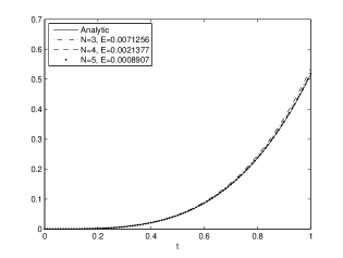
(a) ${{}_{0}I_{t}^{0.5}}(t^{3})$

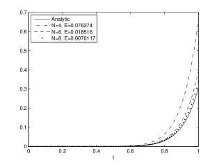
(b) ${{}_{0}I_{t}^{0.5}}(t^{10})$

Figure 6.1: Analytic versus numerical approximation for a fixed $n$.

Secondly, we apply our procedure to the transcendental functions $x_{3}(t)=e^{t}$ and $x_{4}(t)=\sin(t)$. Simple calculations give

$${{}_{0}I_{t}^{0.5}}x_{3}(t)=\sqrt{t}\sum_{k=0}^{\infty}\frac{t^{k}}{\Gamma(k+1.5)}\ \mbox{ and }\ {{}_{0}I_{t}^{0.5}}x_{4}(t)=\sqrt{t}\sum_{k=0}^{\infty}\frac{(-1)^{k}t^{2k+1}}{\Gamma(2k+2.5)}.$$

Figures 6.2(a) and 6.2(b) show the numerical results for each approximation, with $n=3$. We see that for a small value of $N$ one already obtains a good approximation for each function.

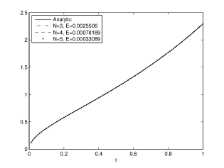
(a) ${{}_{0}I_{t}^{0.5}}(e^{t})$

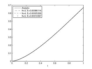
(b) ${{}_{0}I_{t}^{0.5}}(\sin(t))$

Figure 6.2: Analytic versus numerical approximation for a fixed $n$.

For analytical functions, we may apply the well-known formula (6.2). In Figure 6.3 we show the results of approximating with (6.2), $N=1,2,3$, for functions $x_{3}(t)$ and $x_{4}(t)$. We remark that, when we consider expansions up to the second derivative, i.e., the cases $n=3$ as in (6.3) and expansion (6.2) with $N=2$, we obtain a better accuracy using our approximation (6.3) even for a small value of $N$.

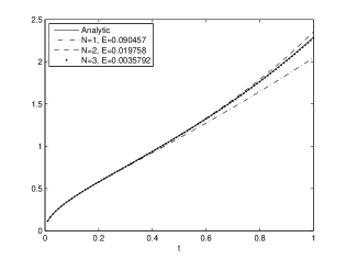
(a) ${{}_{0}I_{t}^{0.5}}(e^{t})$

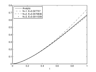
(b) ${{}_{0}I_{t}^{0.5}}(\sin(t))$

Figure 6.3: Numerical approximation using (6.2) of previous literature.

Another way to approximate fractional integrals is to fix $N$ and consider several sizes for the decomposition, i.e., letting $n$ to vary. Let us consider the two test functions $x_{1}(t)=t^{3}$ and $x_{2}(t)=t^{10}$, with $t\in[0,1]$ as before. In both cases we consider the first three approximations of the fractional integral, i.e., for $n=1,2,3$. For the first function we fix $N=3$, for the second one we choose $N=8$. Figures 6.4(a) and 6.4(b) show the numerical results. As expected, for a greater value of $n$ the error decreases.

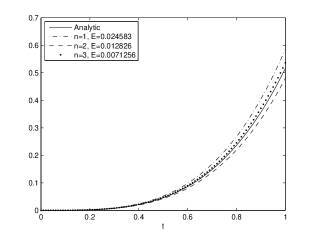
(a) ${{}_{0}I_{t}^{0.5}}(t^{3})$

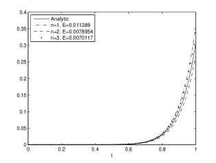
(b) ${{}_{0}I_{t}^{0.5}}(t^{10})$

Figure 6.4: Analytic versus numerical approximation for a fixed $N$.

We mentioned before that although the terms $A_{i}$ are all equal to zero, for $i\in\{0,\ldots,n-1\}$, we consider them in the decomposition formula. Indeed, after we truncate the sum, the error is lower. This is illustrated in Figures 6.5(a) and 6.5(b), where we study the approximations for ${{}_{0}I_{t}^{0.5}}x_{1}(t)$ and ${{}_{0}I_{t}^{0.5}}x_{2}(t)$ with $A_{i}\not=0$ and $A_{i}=0$.

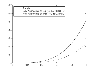
(a) ${{}_{0}I_{t}^{0.5}}(t^{3})$

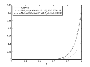
(b) ${{}_{0}I_{t}^{0.5}}(t^{10})$

Figure 6.5: Comparison of approximation (6.3) and approximation with $A_{i}=0$.

6.1.4 Applications to fractional integral equations

In this section we show how the proposed approximations can be applied to solve a fractional integral equation (Example 41) which depends on the left Riemann–Liouville fractional integral. The main idea is to rewrite the initial problem by replacing the fractional integrals by an expansion of type (6.1) or (6.6), and thus getting a problem involving integer-order derivatives, which can be solved by standard techniques.

Example 41.

Consider the following fractional system:

$$\left\{\begin{array}[]{l}{{}_{0}I_{t}^{0.5}}x(t)=\frac{\Gamma(4.5)}{24}t^{4}\\ x(0)=0.\end{array}\right.$$ (6.14)

Since ${{}_{0}I_{t}^{0.5}}t^{3.5}=\frac{\Gamma(4.5)}{24}t^{\alpha}$, the function $t\mapsto t^{3.5}$ is a solution to problem (6.14).

To provide a numerical method to solve such type of systems, we replace the fractional integral by approximations (6.2) and (6.10), for a suitable order. We remark that the order of approximation, $N$ in (6.2) and $n$ in (6.10), are restricted by the number of given initial or boundary conditions. Since (6.14) has one initial condition, in order to solve it numerically, we will consider the expansion for the fractional integral up to the first derivative, i.e., $N=1$ in (6.2) and $n=2$ in (6.10). The order $N$ in (6.10) can be freely chosen.

Applying approximation (6.2), with $\alpha=0.5$, we transform (6.14) into the initial value problem

$$\left\{\begin{array}[]{l}1.1285t^{0.5}x(t)-0.3761t^{1.5}\dot{x}(t)=\frac{\Gamma(4.5)}{24}t^{4},\\ x(0)=0,\end{array}\right.$$

which is a first order ODE. The solution is shown in Figure 6.6(a). It reveals that the approximation remains close to the exact solution for a short time and diverges drastically afterwards. Since we have no extra information, we cannot increase the order of approximation to proceed.

To use expansion (6.6), we rewrite the problem as a standard one, depending only on a derivative of first order. The approximated system that we must solve is

$$\left\{\begin{array}[]{l}A_{0}(0.5,N)t^{0.5}x(t)+A_{1}(0.5,N)t^{1.5}\dot{x}(t)+\sum_{p=2}^{N}B(0.5,p)t^{1.5-p}V_{p}(t)=\frac{\Gamma(4.5)}{24}t^{4},\\ \dot{V}_{p}(t)=(p-1)t^{p-2}x(t),\quad p=2,3,\ldots,N,\\ x(0)=0,\\ V_{p}(0)=0,\quad p=2,3,\ldots,N,\\ \end{array}\right.$$

where $A_{0}$ and $A_{1}$ are given as in (6.11) and $B$ is given by Theorem 39. Here, by increasing $N$, we get better approximations to the fractional integral and we expect more accurate solutions to the original problem (6.14). For $N=2$ and $N=3$ we transform the resulting system of ordinary differential equations to a second and a third order differential equation, respectively. Finally, we solve them using the Maple built in function dsolve. For example, for $N=2$ the second-order equation takes the form

$$\left\{\begin{array}[]{l}\ddot{V}_{2}(t)=\frac{6}{t}\dot{V}_{2}(t)+\frac{6}{t^{2}}V_{2}(t)-5.1542t^{2.5}\\ V_{2}(0)=0\\ \dot{V}_{2}(0)=x(0)=0,\end{array}\right.$$

and the solution is $x(t)=\dot{V}_{2}(t)=1.34t^{3.5}$. In Figure 6.6(b) we compare the exact solution with numerical approximations for two values of $N$.

(a) Approximation by (6.2).

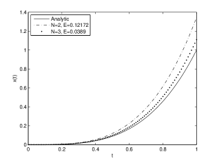
(b) Approximation by (6.10).

Figure 6.6: Analytic versus numerical solution to problem (6.14).

6.2 Hadamard fractional integrals

6.2.1 Approximation by a sum of integer-order derivatives

For an arbitrary $\alpha>0$ we refer the reader to [65, Theorem 3.2]. If a function $x$ admits derivatives of any order, then expansion formulas for the Hadamard fractional integrals and derivatives of $x$, in terms of its integer-order derivatives, are given in [35, Theorem 17]:

$${{}_{0}\mathcal{I}_{t}^{\alpha}}x(t)=\sum_{k=0}^{\infty}S(-\alpha,k)t^{k}x^{(k)}(t)$$

and

$${{}_{0}\mathcal{D}_{t}^{\alpha}}x(t)=\sum_{k=0}^{\infty}S(\alpha,k)t^{k}x^{(k)}(t),$$

where

$$S(\alpha,k)=\frac{1}{k!}\sum_{j=1}^{k}(-1)^{k-j}{k\choose j}j^{\alpha}$$

is the Stirling function.

6.2.2 Approximation using moments of a function

In this section we consider the class of differentiable functions up to order $n+1$, $x\in C^{n+1}[a,b]$, and deduce expansion formulas for the Hadamard fractional integrals in terms of $x^{(i)}(\cdot)$, for $i\in\{0,\ldots,n\}$. Before presenting the result in its full extension, we briefly explain the techniques involved for the particular case $n=2$. To that purpose, let $x\in C^{3}[a,b]$. Integrating by parts three times, we obtain

$$\begin{array}[]{ll}{{}_{a}\mathcal{I}_{t}^{\alpha}}x(t)&=\displaystyle-\frac{1}{\Gamma(\alpha)}\int_{a}^{t}-\frac{1}{\tau}\left(\ln\frac{t}{\tau}\right)^{\alpha-1}x(\tau)d\tau\\ &=\displaystyle\frac{1}{\Gamma(\alpha+1)}\left(\ln\frac{t}{a}\right)^{\alpha}x(a)-\frac{1}{\Gamma(\alpha+1)}\int_{a}^{t}-\frac{1}{\tau}\left(\ln\frac{t}{\tau}\right)^{\alpha}\tau\dot{x}(\tau)d\tau\\ &=\displaystyle\frac{1}{\Gamma(\alpha+1)}\left(\ln\frac{t}{a}\right)^{\alpha}x(a)+\frac{1}{\Gamma(\alpha+2)}\left(\ln\frac{t}{a}\right)^{\alpha+1}a\dot{x}(a)\\ &\quad\displaystyle-\frac{1}{\Gamma(\alpha+2)}\int_{a}^{t}-\frac{1}{\tau}\left(\ln\frac{t}{\tau}\right)^{\alpha+1}(\tau\dot{x}(\tau)+\tau^{2}\ddot{x}(\tau))d\tau\\ &=\displaystyle\frac{1}{\Gamma(\alpha+1)}\left(\ln\frac{t}{a}\right)^{\alpha}x(a)+\frac{1}{\Gamma(\alpha+2)}\left(\ln\frac{t}{a}\right)^{\alpha+1}a\dot{x}(a)\\ &\displaystyle\quad+\frac{1}{\Gamma(\alpha+3)}\left(\ln\frac{t}{a}\right)^{\alpha+2}(a\dot{x}(a)+a^{2}\ddot{x}(a))\\ &\quad+\displaystyle\frac{1}{\Gamma(\alpha+3)}\int_{a}^{t}\left(\ln\frac{t}{\tau}\right)^{\alpha+2}(\dot{x}(\tau)+3\tau\ddot{x}(\tau)+\tau^{2}\dddot{x}(\tau))d\tau.\end{array}$$

On the other hand, using the binomial theorem, we have

$$\begin{array}[]{ll}\displaystyle\left(\ln\frac{t}{\tau}\right)^{\alpha+2}&=\displaystyle\left(\ln\frac{t}{a}\right)^{\alpha+2}\left(1-\frac{\ln\frac{\tau}{a}}{\ln\frac{t}{a}}\right)^{\alpha+2}\\ &=\displaystyle\left(\ln\frac{t}{a}\right)^{\alpha+2}\sum_{p=0}^{\infty}\frac{\Gamma(p-\alpha-2)}{\Gamma(-\alpha-2)p!}\cdot\frac{\left(\ln\frac{\tau}{a}\right)^{p}}{\left(\ln\frac{t}{a}\right)^{p}}.\end{array}$$

This series converges since $\tau\in[a,t]$ and $\alpha+2>0$. Combining these formulas, we get

$${{}_{a}\mathcal{I}_{t}^{\alpha}}x(t) = \frac{x(a)}{\Gamma(\alpha+1)}\left(\ln\frac{t}{a}\right)^{\alpha}+\frac{a\dot{x}(a)}{\Gamma(\alpha+2)}\left(\ln\frac{t}{a}\right)^{\alpha+1}+\frac{a\dot{x}(a)+a^{2}\ddot{x}(a)}{\Gamma(\alpha+3)}\left(\ln\frac{t}{a}\right)^{\alpha+2}$$

$$+\frac{1}{\Gamma(\alpha+3)}\left(\ln\frac{t}{a}\right)^{\alpha+2}\sum_{p=0}^{\infty}\Gamma_{0}(\alpha,p,t)\int_{a}^{t}\left(\ln\frac{\tau}{a}\right)^{p}\left(\dot{x}(\tau)+3\tau\ddot{x}(\tau)+\tau^{2}\dddot{x}(\tau)\right)d\tau,$$

where

$$\Gamma_{i}(\alpha,p,t)=\frac{\Gamma(p-\alpha-2)}{\Gamma(-\alpha-2+i)(p-i)!\left(\ln\frac{t}{a}\right)^{p}}.$$

Now, split the series into the two cases $p=0$ and $p=1\ldots\infty$, and integrate by parts the second one. We obtain

$$\begin{array}[]{ll}{{}_{a}\mathcal{I}_{t}^{\alpha}}x(t)&=\displaystyle\frac{1}{\Gamma(\alpha+1)}\left(\ln\frac{t}{a}\right)^{\alpha}x(a)+\frac{1}{\Gamma(\alpha+2)}\left(\ln\frac{t}{a}\right)^{\alpha+1}a\dot{x}(a)\\ &\displaystyle\quad+\frac{1}{\Gamma(\alpha+3)}\left(\ln\frac{t}{a}\right)^{\alpha+2}(t\dot{x}(t)+t^{2}\ddot{x}(t))\left[1+\sum_{p=1}^{\infty}\frac{\Gamma(p-\alpha-2)}{\Gamma(-\alpha-2)p!}\right]\\ &\displaystyle\quad+\frac{1}{\Gamma(\alpha+2)}\left(\ln\frac{t}{a}\right)^{\alpha+2}\sum_{p=1}^{\infty}\Gamma_{1}(\alpha,p,t)\int_{a}^{t}\left(\ln\frac{\tau}{a}\right)^{p-1}(\dot{x}(\tau)+\tau\ddot{x}(\tau))d\tau.\end{array}$$

Repeating this procedure two more times, we obtain the following:

$$\begin{array}[]{ll}{{}_{a}\mathcal{I}_{t}^{\alpha}}x(t)&=\displaystyle\frac{1}{\Gamma(\alpha+1)}\left(\ln\frac{t}{a}\right)^{\alpha}x(t)\left[1+\sum_{p=3}^{\infty}\frac{\Gamma(p-\alpha-2)}{\Gamma(-\alpha)(p-2)!}\right]\\ &\displaystyle\quad+\frac{1}{\Gamma(\alpha+2)}\left(\ln\frac{t}{a}\right)^{\alpha+1}t\dot{x}(t)\left[1+\sum_{p=2}^{\infty}\frac{\Gamma(p-\alpha-2)}{\Gamma(-\alpha-1)(p-1)!}\right]\\ &\displaystyle\quad+\frac{1}{\Gamma(\alpha+3)}\left(\ln\frac{t}{a}\right)^{\alpha+2}(t\dot{x}(t)+t^{2}\ddot{x}(t))\left[1+\sum_{p=1}^{\infty}\frac{\Gamma(p-\alpha-2)}{\Gamma(-\alpha-2)p!}\right]\\ &\displaystyle\quad+\frac{1}{\Gamma(\alpha)}\left(\ln\frac{t}{a}\right)^{\alpha+2}\sum_{p=3}^{\infty}\frac{\Gamma(p-\alpha-2)}{\Gamma(-\alpha+1)(p-3)!\left(\ln\frac{t}{a}\right)^{p}}\int_{a}^{t}\left(\ln\frac{\tau}{a}\right)^{p-3}\frac{x(\tau)}{\tau}d\tau,\end{array}$$

or, in a more concise way,

$$\begin{array}[]{ll}{{}_{a}\mathcal{I}_{t}^{\alpha}}x(t)&=\displaystyle A_{0}(\alpha)\left(\ln\frac{t}{a}\right)^{\alpha}x(t)+A_{1}(\alpha)\left(\ln\frac{t}{a}\right)^{\alpha+1}t\dot{x}(t)\\ &\quad\displaystyle+A_{2}(\alpha)\left(\ln\frac{t}{a}\right)^{\alpha+2}(t\dot{x}(t)+t^{2}\ddot{x}(t))+\sum_{p=3}^{\infty}B(\alpha,p)\left(\ln\frac{t}{a}\right)^{\alpha+2-p}V_{p}(t),\end{array}$$

with

$$\begin{array}[]{ll}A_{0}(\alpha)&=\displaystyle\frac{1}{\Gamma(\alpha+1)}\left[1+\sum_{p=3}^{\infty}\frac{\Gamma(p-\alpha-2)}{\Gamma(-\alpha)(p-2)!}\right],\\ A_{1}(\alpha)&=\displaystyle\frac{1}{\Gamma(\alpha+2)}\left[1+\sum_{p=2}^{\infty}\frac{\Gamma(p-\alpha-2)}{\Gamma(-\alpha-1)(p-1)!}\right],\\ A_{2}(\alpha)&=\displaystyle\frac{1}{\Gamma(\alpha+3)}\left[1+\sum_{p=1}^{\infty}\frac{\Gamma(p-\alpha-2)}{\Gamma(-\alpha-2)p!}\right],\end{array}$$

$$B(\alpha,p)=\displaystyle\frac{\Gamma(p-\alpha-2)}{\Gamma(\alpha)\Gamma(1-\alpha)(p-2)!},$$ (6.15)

and

$$V_{p}(t)=\int_{a}^{t}(p-2)\left(\ln\frac{\tau}{a}\right)^{p-3}\frac{x(\tau)}{\tau}d\tau,$$ (6.16)

where we assume the series and the integral $V_{p}$ to be convergent.

Remark 42.

When useful, namely on fractional differential and integral equations, we can define $V_{p}$ as in (6.16) by the solution of the system

$$\left\{\begin{array}[]{l}\dot{V_{p}}(t)=\displaystyle(p-2)\left(\ln\frac{t}{a}\right)^{p-3}\frac{x(t)}{t}\\ V_{p}(a)=0,\end{array}\right.$$

for all $p=3,4,\ldots$

We now discuss the convergence of the series involved in the definitions of $A_{i}(\alpha)$, for $i\in\{0,1,2\}$. Simply observe that

$$\sum_{p=3-i}^{\infty}\frac{\Gamma(p-\alpha-2)}{\Gamma(-\alpha-i)(p-2+i)!}={{}_{1}F_{0}}(-\alpha-i,1)-1,$$

and ${{}_{1}F_{0}}(a,x)$ converges absolutely when $|x|=1$ if $a<0$ ([18, Theorem 2.1.2]).

For numerical purposes, only finite sums are considered, and thus the Hadamard left fractional integral is approximated by the decomposition

$$\begin{array}[]{ll}{{}_{a}\mathcal{I}_{t}^{\alpha}}x(t)&\approx\displaystyle A_{0}(\alpha,N)\left(\ln\frac{t}{a}\right)^{\alpha}x(t)+A_{1}(\alpha,N)\left(\ln\frac{t}{a}\right)^{\alpha+1}t\dot{x}(t)\\ &\quad\displaystyle+A_{2}(\alpha,N)\left(\ln\frac{t}{a}\right)^{\alpha+2}(t\dot{x}(t)+t^{2}\ddot{x}(t))+\sum_{p=3}^{N}B(\alpha,p)\left(\ln\frac{t}{a}\right)^{\alpha+2-p}V_{p}(t),\end{array}$$ (6.17)

with

$$\begin{array}[]{ll}A_{0}(\alpha,N)&=\displaystyle\frac{1}{\Gamma(\alpha+1)}\left[1+\sum_{p=3}^{N}\frac{\Gamma(p-\alpha-2)}{\Gamma(-\alpha)(p-2)!}\right],\\ A_{1}(\alpha,N)&=\displaystyle\frac{1}{\Gamma(\alpha+2)}\left[1+\sum_{p=2}^{N}\frac{\Gamma(p-\alpha-2)}{\Gamma(-\alpha-1)(p-1)!}\right],\\ A_{2}(\alpha,N)&=\displaystyle\frac{1}{\Gamma(\alpha+3)}\left[1+\sum_{p=1}^{N}\frac{\Gamma(p-\alpha-2)}{\Gamma(-\alpha-2)p!}\right],\end{array}$$

$B(\alpha,p)$ and $V_{p}(t)$ as in (6.15)–(6.16), and $N\geq 3$.

Following similar arguments as done for $n=2$, we can prove the general case with an expansion up to the derivative of order $n$. First, we introduce a notation. Given $k\in\mathbb{N}\cup\{0\}$, we define the sequences $x_{k,0}(t)$ and $x_{k,1}(t)$ recursively by the formulas

$$x_{0,0}(t)=x(t)\mbox{ and }x_{k+1,0}(t)=t\frac{d}{dt}x_{k,0}(t),\mbox{ for }k\in\mathbb{N}\cup\{0\},$$

and

$$x_{0,1}(t)=\dot{x}(t)\mbox{ and }x_{k+1,1}(t)=\frac{d}{dt}(tx_{k,1}(t)),\mbox{ for }k\in\mathbb{N}\cup\{0\}.$$

Theorem 43.

Let $n\in\mathbb{N}$, $0<a<b$ and $x:[a,b]\to\mathbb{R}$ be a function of class $C^{n+1}$. Then,

$${{}_{a}\mathcal{I}_{t}^{\alpha}}x(t)=\sum_{i=0}^{n}A_{i}(\alpha)\left(\ln\frac{t}{a}\right)^{\alpha+i}x_{i,0}(t)+\sum_{p=n+1}^{\infty}B(\alpha,p)\left(\ln\frac{t}{a}\right)^{\alpha+n-p}V_{p}(t)$$

with

$$\begin{array}[]{ll}A_{i}(\alpha)&=\displaystyle\frac{1}{\Gamma(\alpha+i+1)}\left[1+\sum_{p=n-i+1}^{\infty}\frac{\Gamma(p-\alpha-n)}{\Gamma(-\alpha-i)(p-n+i)!}\right],\\[12.0pt] B(\alpha,p)&=\displaystyle\frac{\Gamma(p-\alpha-n)}{\Gamma(\alpha)\Gamma(1-\alpha)(p-n)!},\\[12.0pt] V_{p}(t)&=\displaystyle\int_{a}^{t}(p-n)\left(\ln\frac{\tau}{a}\right)^{p-n-1}\frac{x(\tau)}{\tau}d\tau.\end{array}$$

Proof.

Applying integration by parts repeatedly and the binomial formula, we arrive to

$$\begin{array}[]{ll}{{}_{a}\mathcal{I}_{t}^{\alpha}}x(t)&=\displaystyle\sum_{i=0}^{n}\frac{1}{\Gamma(\alpha+i+1)}\left(\ln\frac{t}{a}\right)^{\alpha+i}x_{i,0}(a)\\ &\quad\displaystyle+\frac{1}{\Gamma(\alpha+n+1)}\left(\ln\frac{t}{a}\right)^{\alpha+n}\sum_{p=0}^{\infty}\frac{\Gamma(p-\alpha-n)}{\Gamma(-\alpha-n)p!\left(\ln\frac{t}{a}\right)^{p}}\int_{a}^{t}\left(\ln\frac{\tau}{a}\right)^{p}x_{n,1}(\tau)d\tau.\end{array}$$

To achieve the expansion formula, we repeat the same procedure as for the case $n=2$: we split the sum into two parts (the first term plus the remaining) and integrate by parts the second one. The convergence of the series $A_{i}(\alpha)$ is ensured by the relation

$$\sum_{p=n-i+1}^{\infty}\frac{\Gamma(p-\alpha-n)}{\Gamma(-\alpha-i)(p-n+i)!}={{}_{1}F_{0}}(-\alpha-i,1)-1.$$

∎

An estimation for the error bound is given in Section 6.3.

Similarly to what was done with the left fractional integral, we can also expand the right Hadamard fractional integral.

Theorem 44.

Let $n\in\mathbb{N}$, $0<a<b$ and $x:[a,b]\to\mathbb{R}$ be a function of class $C^{n+1}$. Then,

$${{}_{t}\mathcal{I}_{b}^{\alpha}}x(t)=\sum_{i=0}^{n}A_{i}(\alpha)\left(\ln\frac{b}{t}\right)^{\alpha+i}x_{i,0}(t)+\sum_{p=n+1}^{\infty}B(\alpha,p)\left(\ln\frac{b}{t}\right)^{\alpha+n-p}W_{p}(t)$$

with

$$\begin{array}[]{ll}A_{i}(\alpha)&=\displaystyle\frac{(-1)^{i}}{\Gamma(\alpha+i+1)}\left[1+\sum_{p=n-i+1}^{\infty}\frac{\Gamma(p-\alpha-n)}{\Gamma(-\alpha-i)(p-n+i)!}\right],\\ B(\alpha,p)&=\displaystyle\frac{\Gamma(p-\alpha-n)}{\Gamma(\alpha)\Gamma(1-\alpha)(p-n)!},\\ W_{p}(t)&=\displaystyle\int_{t}^{b}(p-n)\left(\ln\frac{b}{\tau}\right)^{p-n-1}\frac{x(\tau)}{\tau}d\tau.\end{array}$$

Remark 45.

Analogously to what was done for the left fractional integral, one can consider an approximation for the right Hadamard fractional integral by considering finite sums in the expansion obtained in Theorem 44.

6.2.3 Examples

We obtained approximation formulas for the Hadamard fractional integrals. The error caused by such decompositions is given later in Section 6.3. In this section we study several cases, comparing the solution with the approximations. To gather more information on the accuracy, we evaluate the error using the distance

$$E=\sqrt{\int_{a}^{b}\left({{}_{a}\mathcal{I}_{t}^{\alpha}}x(t)-\tilde{{{}_{a}\mathcal{I}_{t}^{\alpha}}}x(t)\right)^{2}dt},$$

where $\tilde{{{}_{a}\mathcal{I}_{t}^{\alpha}}}x(t)$ is the approximated value.

To begin with, we consider $\alpha=0.5$ and functions $x_{1}(t)=\ln t$ and $x_{2}(t)=1$ with $t\in[1,10]$. Then,

$${{}_{1}\mathcal{I}_{t}^{0.5}}x_{1}(t)=\frac{\sqrt{\ln^{3}t}}{\Gamma(2.5)}\mbox{ and }{{}_{1}\mathcal{I}_{t}^{0.5}}x_{2}(t)=\frac{\sqrt{\ln t}}{\Gamma(1.5)}$$

(cf. [66, Property 2.24]). We consider the expansion formula for $n=2$ as in (6.17) for both cases. We obtain then the approximations

$${{}_{1}\mathcal{I}_{t}^{0.5}}x_{1}(t)\approx\left[A_{0}(0.5,N)+A_{1}(0.5,N)+\sum_{p=3}^{N}B(0.5,p)\frac{p-2}{p-1}\right]\sqrt{\ln^{3}t}$$

and

$${{}_{1}\mathcal{I}_{t}^{0.5}}x_{2}(t)\approx\left[A_{0}(0.5,N)+\sum_{p=3}^{N}B(0.5,p)\right]\sqrt{\ln t}.$$

The results are exemplified in Figures 6.7(a) and 6.7(b). As can be seen, the value $N=3$ is enough in order to obtain a good accuracy in the sense of the error function.

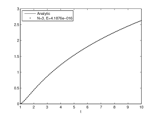
(a) ${{}_{1}\mathcal{I}_{t}^{0.5}}(\ln t)$

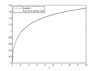
(b) ${{}_{1}\mathcal{I}_{t}^{0.5}}(1)$

Figure 6.7: Analytic vs. numerical approximation for $n=2$.

We now test the approximation on the power functions $x_{3}(t)=t^{4}$ and $x_{4}(t)=t^{9}$, with $t\in[1,2]$. Observe first that

$${{}_{1}\mathcal{I}_{t}^{0.5}}(t^{k})=\frac{1}{\Gamma(0.5)}\int_{1}^{t}\left(\ln\frac{t}{\tau}\right)^{-0.5}\tau^{k-1}d\tau=\frac{t^{k}}{\Gamma(0.5)}\int_{0}^{\ln t}\xi^{-0.5}e^{-\xi k}d\xi$$

by the change of variables $\xi=\ln\frac{t}{\tau}$. In our cases,

$${{}_{1}\mathcal{I}_{t}^{0.5}}(t^{4})\approx\frac{0.8862269255}{\Gamma(0.5)}t^{4}\mbox{erf}(2\sqrt{\ln t})\mbox{ and }{{}_{1}\mathcal{I}_{t}^{0.5}}(t^{9})\approx\frac{0.5908179503}{\Gamma(0.5)}t^{9}\mbox{erf}(3\sqrt{\ln t}),$$

where $\mbox{erf}(\cdot)$ is the error function. In Figures 6.8(a) and 6.8(b) we show approximations for several values of $N$. We mention that, as $N$ increases, the error decreases and thus we obtain a better approximation.

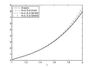
(a) ${{}_{1}\mathcal{I}_{t}^{0.5}}(t^{4})$

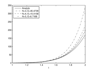
(b) ${{}_{1}\mathcal{I}_{t}^{0.5}}(t^{9})$

Figure 6.8: Analytic vs. numerical approximation for $n=2$.

Another way to obtain different expansion formulas is to vary $n$. To exemplify, we choose the previous test functions $x_{i}$, for $i=1,2,3,4$, and consider the cases $n=2,3,4$ with $N=5$ fixed. The results are shown in Figures 6.9(a), 6.9(b), 6.9(c) and 6.9(d). Observe that as $n$ increases, the error may increase. This can be easily explained by analysis of the error formula, and the values of the sequence $x_{(k,0)}$ involved. For example, for $x_{4}$ we have $x_{(k,0)}(t)=9^{k}t^{9}$, for $k=0\ldots,n$. This suggests that, when we increase the value of $n$ and the function grows fast, in order to obtain a better accuracy on the method, the value of $N$ should also increase.

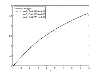
(a) ${{}_{1}\mathcal{I}_{t}^{0.5}}(\ln t)$

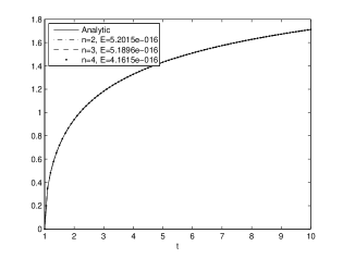
(b) ${{}_{1}\mathcal{I}_{t}^{0.5}}(1)$

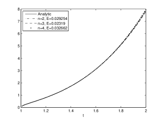
(c) ${{}_{1}\mathcal{I}_{t}^{0.5}}(t^{4})$

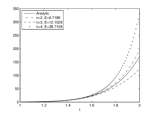
(d) ${{}_{1}\mathcal{I}_{t}^{0.5}}(t^{9})$

Figure 6.9: Analytic vs. numerical approximation for $n=2,3,4$ and $N=5$.

6.3 Error analysis

In the previous section we deduced an approximation formula for the left Riemann–Liouville fractional integral (Eq. (6.10)). The order of magnitude of the coefficients that we ignore during this procedure is small for the examples that we have chosen (Tables 6.1 and 6.2). The aim of this section is to obtain an estimation for the error, when considering sums up to order $N$. We proved that

$${{}_{a}I_{t}^{\alpha}}x(t)=\frac{(t-a)^{\alpha}}{\Gamma(\alpha+1)}x(a)+\cdots+\frac{(t-a)^{\alpha+n-1}}{\Gamma(\alpha+n)}x^{(n-1)}(a)\\ +\frac{(t-a)^{\alpha+n-1}}{\Gamma(\alpha+n)}\int_{a}^{t}\left(1-\frac{\tau-a}{t-a}\right)^{\alpha+n-1}x^{(n)}(\tau)d\tau.$$

Expanding up to order $N$ the binomial, we get

$$\left(1-\frac{\tau-a}{t-a}\right)^{\alpha+n-1}=\sum_{p=0}^{N}\frac{\Gamma(p-\alpha-n+1)}{\Gamma(1-\alpha-n)\,p!}\left(\frac{\tau-a}{t-a}\right)^{p}+R_{N}(\tau),$$

where

$$R_{N}(\tau)=\sum_{p=N+1}^{\infty}\frac{\Gamma(p-\alpha-n+1)}{\Gamma(1-\alpha-n)\,p!}\left(\frac{\tau-a}{t-a}\right)^{p}.$$

Since $\tau\in[a,t]$, we easily deduce an upper bound for $R_{N}(\tau)$:

$$\begin{split}\left|R_{N}(\tau)\right|&\leq\sum_{p=N+1}^{\infty}\left|\frac{\Gamma(p-\alpha-n+1)}{\Gamma(1-\alpha-n)\,p!}\right|=\sum_{p=N+1}^{\infty}\left|\binom{\alpha+n-1}{p}\right|\leq\sum_{p=N+1}^{\infty}\frac{e^{(\alpha+n-1)^{2}+\alpha+n-1}}{p^{\alpha+n}}\\ &\leq\int_{N}^{\infty}\frac{e^{(\alpha+n-1)^{2}+\alpha+n-1}}{p^{\alpha+n}}dp=\frac{e^{(\alpha+n-1)^{2}+\alpha+n-1}}{(\alpha+n-1)N^{\alpha+n-1}}.\end{split}$$

Thus, we obtain an estimation for the truncation error $E_{tr}(\cdot)$:

$$\left|E_{tr}(t)\right|\leq L_{n}\frac{(t-a)^{\alpha+n}e^{(\alpha+n-1)^{2}+\alpha+n-1}}{\Gamma(\alpha+n)(\alpha+n-1)N^{\alpha+n-1}},$$

where $\displaystyle L_{n}=\max_{\tau\in[a,t]}|x^{(n)}(\tau)|$.

We proceed with an estimation for the error on the approximation for the Hadamard fractional integral. We have proven before that

$${{}_{a}\mathcal{I}_{t}^{\alpha}}x(t) = \frac{x(a)}{\Gamma(\alpha+1)}\left(\ln\frac{t}{a}\right)^{\alpha}+\frac{a\dot{x}(a)}{\Gamma(\alpha+2)}\left(\ln\frac{t}{a}\right)^{\alpha+1}+\frac{(a\dot{x}(a)+a^{2}\ddot{x}(a))}{\Gamma(\alpha+3)}\left(\ln\frac{t}{a}\right)^{\alpha+2}$$

$$+\frac{1}{\Gamma(\alpha+3)}\left(\ln\frac{t}{a}\right)^{\alpha+2}\int_{a}^{t}\sum_{p=0}^{\infty}\Gamma_{1}(\alpha,p,t)(\dot{x}(\tau)+3\tau\ddot{x}(\tau)+\tau^{2}\dddot{x}(\tau))d\tau.$$

When we consider finite sums up to order $N$, the error is given by

$$\left|E_{tr}(t)\right|=\left|\frac{1}{\Gamma(\alpha+3)}\left(\ln\frac{t}{a}\right)^{\alpha+2}\int_{a}^{t}R_{N}(\tau)(\dot{x}(\tau)+3\tau\ddot{x}(\tau)+\tau^{2}\dddot{x}(\tau))d\tau\right|$$

with

$$R_{N}(\tau)=\sum_{p=N+1}^{\infty}\frac{\Gamma(p-\alpha-2)}{\Gamma(-\alpha-2)p!}\frac{\left(\ln\frac{\tau}{a}\right)^{p}}{\left(\ln\frac{t}{a}\right)^{p}}.$$

Since $\tau\in[a,t]$, we have

$$\begin{array}[]{ll}|R_{N}(\tau)|&\displaystyle\leq\sum_{p=N+1}^{\infty}\left|\binom{\alpha+2}{p}\right|\leq\sum_{p=N+1}^{\infty}\frac{e^{(\alpha+2)^{2}+\alpha+2}}{p^{\alpha+3}}\\ &\displaystyle\leq\int_{N}^{\infty}\frac{e^{(\alpha+2)^{2}+\alpha+2}}{p^{\alpha+3}}dp=\frac{e^{(\alpha+2)^{2}+\alpha+2}}{(\alpha+2)N^{\alpha+2}}.\end{array}$$

Therefore,

$$\left|E_{tr}(t)\right|\leq\frac{e^{(\alpha+2)^{2}+\alpha+2}}{(\alpha+2)N^{\alpha+2}}\frac{\left(\ln\frac{t}{a}\right)^{\alpha+2}}{\Gamma(\alpha+3)}\left[(t-a)L_{1}(t)+3(t-a)^{2}L_{2}(t)+(t-a)^{3}L_{3}(t)\right],$$

where

$$L_{i}(t)=\max_{\tau\in[a,t]}|x^{(i)}(\tau)|,\quad i\in\{1,2,3\}.$$

We remark that the error formula tends to zero as $N$ increases. Moreover, if we consider the approximation

$${{}_{a}\mathcal{I}_{t}^{\alpha}}x(t)\approx\sum_{i=0}^{n}A_{i}(\alpha,N)\left(\ln\frac{t}{a}\right)^{\alpha+i}x_{i,0}(t)+\sum_{p=n+1}^{N}B(\alpha,p)\left(\ln\frac{t}{a}\right)^{\alpha+n-p}V_{p}(t)$$

with $N\geq n+1$ and

$$A_{i}(\alpha,N)=\frac{1}{\Gamma(\alpha+i+1)}\left[1+\sum_{p=n-i+1}^{N}\frac{\Gamma(p-\alpha-n)}{\Gamma(-\alpha-i)(p-n+i)!}\right],$$

then the error is bounded by the expression

$$\left|E_{tr}(t)\right|\leq L_{n}(t)\frac{e^{(\alpha+n)^{2}+\alpha+n}}{\Gamma(\alpha+n+1)(\alpha+n)N^{\alpha+n}}\left(\ln\frac{t}{a}\right)^{\alpha+n}(t-a),$$

where

$$L_{n}(t)=\max_{\tau\in[a,t]}|x_{n,1}(\tau)|.$$

For the right Hadamard integral, the error is bounded by

$$\left|E_{tr}(t)\right|\leq L_{n}(t)\frac{e^{(\alpha+n)^{2}+\alpha+n}}{\Gamma(\alpha+n+1)(\alpha+n)N^{\alpha+n}}\left(\ln\frac{b}{t}\right)^{\alpha+n}(b-t),$$

where

$$L_{n}(t)=\max_{\tau\in[t,b]}|x_{n,1}(\tau)|.$$

Chapter 7 Direct methods

In the presence of fractional operators, the same ideas that were discussed in Section 1.1.3, are applied to discretize the problem. Many works can be found in the literature that use different types of basis functions to establish Ritz-like methods for the fractional calculus of variations and optimal control. Nevertheless, finite differences have got less interest. A brief introduction of using finite differences has been made in [106], which can be regarded as a predecessor to what we call here an Euler-like direct method. A generalization of Leitmann’s direct method can be found in [16], while [75] discusses the Ritz direct method for optimal control problems that can easily be reduced to a problem of the calculus of variations.

7.1 Finite differences for fractional derivatives

Recall the definitions of Grünwald–Letnikov, e.g. (2.1). It exhibits a finite difference nature involving an infinite series. For numerical purposes we need a finite sum in (2.1). Given a grid on $[a,b]$ as $a=t_{0},t_{1},\ldots,t_{n}=b$, where $t_{i}=t_{0}+ih$ for some $h>0$, we approximate the left Riemann–Liouville derivative as

$${{}_{a}D_{t}^{\alpha}}x(t_{i})\approx\frac{1}{h^{\alpha}}\sum_{k=0}^{i}\left(\omega_{k}^{\alpha}\right)x(t_{i}-kh),$$ (7.1)

where $\left(\omega_{k}^{\alpha}\right)=(-1)^{k}\binom{\alpha}{k}=\frac{\Gamma(k-\alpha)}{\Gamma(-\alpha)\Gamma(k+1)}$.

Remark 46.

Similarly, one can approximate the right Riemann–Liouville derivative by

$${{}_{t}D_{b}^{\alpha}}x(t_{i})\approx\frac{1}{h^{\alpha}}\sum_{k=0}^{n-i}\left(\omega_{k}^{\alpha}\right)x(t_{i}+kh).$$ (7.2)

Remark 47.

The Grünwald–Letnikov approximation of Riemann–Liouville is a first order approximation [93], i.e.,

$${{}_{a}D_{t}^{\alpha}}x(t_{i})=\frac{1}{h^{\alpha}}\sum_{k=0}^{i}\left(\omega_{k}^{\alpha}\right)x(t_{i}-kh)+\mathcal{O}(h).$$

Remark 48.

It has been shown that the implicit Euler method solution to a certain fractional partial differential equation based on Grünwald–Letnikov approximation to the fractional derivative, is unstable [82]. Therefore, discretizing fractional derivatives, shifted Grünwald–Letnikov derivatives are used and despite the slight difference they exhibit a stable performance at least for certain cases. The left shifted Grünwald–Letnikov derivative is defined by

$${{}^{sGL}_{\phantom{1}a}D_{t}^{\alpha}}x(t_{i})\approx\frac{1}{h^{\alpha}}\sum_{k=0}^{i}\left(\omega_{k}^{\alpha}\right)x(t_{i}-(k-1)h).$$

Other finite difference approximations can be found in the literature. Specifically, we refer to [41], Diethelm’s backward finite differences formula for Caputo fractional derivative, with $0<\alpha<2$ and $\alpha\neq 1$, that is an approximation of order $\mathcal{O}(h^{2-\alpha})$:

$${{}_{a}^{C}D_{t}^{\alpha}}x(t_{i})\approx\frac{h^{-\alpha}}{\Gamma(2-\alpha)}\sum_{j=0}^{i}a_{i,j}\left(x_{i-j}-\sum_{k=0}^{\lfloor\alpha\rfloor}\frac{(i-j)^{k}h^{k}}{k!}x^{(k)}(a)\right),$$

where

$$a_{i,j}=\left\{\begin{array}[]{ll}1,&\text{if }i=0,\\ (j+1)^{1-\alpha}-2j^{1-\alpha}+(j-1)^{1-\alpha},&\text{if }0<j<i,\\ (1-\alpha)i^{-\alpha}-i^{1-\alpha}+(i-1)^{1-\alpha},&\text{if }j=i.\end{array}\right.$$

7.2 Euler-like direct method for variational problems

7.2.1 Euler’s classic direct method

Euler’s method in the classical theory of the calculus of variations uses finite difference approximations for derivatives and is also referred as the method of finite differences. The basic idea of this method is that instead of considering the values of a functional

$$J[x(\cdot)]=\int_{a}^{b}L(t,x(t),\dot{x}(t))dt$$

with boundary conditions $x(a)=x_{a}$ and $x(b)=x_{b}$, on arbitrary admissible curves, we only track the values at an $n+1$ grid points, $t_{i},~{}i=0,\ldots,n$, of the interested time interval [96]. The functional $J[x(\cdot)]$ is then transformed into a function $\Psi(x(t_{1}),x(t_{2}),\ldots,x(t_{n-1}))$ of the values of the unknown function on mesh points. Assuming $h=t_{i}-t_{i-1}$, $x(t_{i})=x_{i}$ and $\dot{x}_{i}\approx\frac{x_{i}-x_{i-1}}{h}$, one has

$$J[x(\cdot)] \approx \Psi(x_{1},x_{2},\ldots,x_{n-1})=h\sum_{i=1}^{n}L\left(t_{i},x_{i},\frac{x_{i}-x_{i-1}}{h}\right),$$

$$x_{0}=x_{a},\quad x_{n}=x_{b}.$$

The desired values of $x_{i}$, $i=1,\ldots,n-1$, are the extremum of the multi-variable function $\Psi$ which is the solution to the system

$$\frac{\partial\Psi}{\partial x_{i}}=0,\quad i=1,\ldots,n-1.$$

The fact that only two terms in the sum, $(i-1)$th and $i$th, depend on $x_{i}$ makes it rather easy to find the extremum of $\Psi$ solving a system of algebraic equations. For each $n$, we obtain a polygonal line which is an approximate solution of the original problem. It has been shown that passing to the limit as $h\rightarrow 0$, the linear system corresponding to finding the extremum of $\Psi$ is equivalent to the Euler–Lagrange equation for problem [122].

7.2.2 Euler-like direct method

As mentioned earlier, we consider a simple version of fractional variational problems where the fractional term has a Riemann–Liouville derivative on a finite time interval $[a,b]$. The boundary conditions are given and we approximate the derivative using Grünwald–Letnikov approximation given by (7.1). In this context, we discretize the functional in (3.1) using a simple quadrature rule on the mesh points, $a=t_{0},t_{1},,\ldots,t_{n}=b$, with $h=\frac{b-a}{n}$. The goal is to find the values $x_{1},\ldots,x_{n-1}$ of the unknown function $x(\cdot)$ at the points $t_{i}$, $i=1,\ldots,n-1$. The values of $x_{0}$ and $x_{n}$ are given. Applying the quadrature rule gives

$$J[x(\cdot)] = \sum_{i=1}^{n}\int_{t_{i-1}}^{t_{i}}L(t_{i},x_{i},{{}_{a}D_{t_{i}}^{\alpha}}x_{i})dt\approx\sum_{i=1}^{n}hL(t_{i},x_{i},{{}_{a}D_{t_{i}}^{\alpha}}x_{i}),$$

and by approximating the fractional derivatives at mesh points using (7.1) we have

$$J[x(\cdot)]\approx\sum_{i=1}^{n}hL\left(t_{i},x_{i},\frac{1}{h^{\alpha}}\sum_{k=0}^{i}\left(\omega_{k}^{\alpha}\right)x_{i-k}\right).$$ (7.3)

Hereafter the procedure is the same as in classical case. The right-hand-side of (7.3) can be regarded as a function $\Psi$ of $n-1$ unknowns $\mathbf{x}=(x_{1},x_{2},\ldots,x_{n-1})$,

$$\Psi(\mathbf{x})=\sum_{i=1}^{n}hL\left(t_{i},x_{i},\frac{1}{h^{\alpha}}\sum_{k=0}^{i}\left(\omega_{k}^{\alpha}\right)x_{i-k}\right).$$ (7.4)

To find an extremum for $\Psi$, one has to solve the following system of algebraic equations:

$$\frac{\partial\Psi}{\partial x_{i}}=0,\qquad i=1,\ldots,n-1.$$ (7.5)

Unlike the classical case, all terms, starting from $i$th term, in (7.4) depend on $x_{i}$ and we have

$$\frac{\partial\Psi}{\partial x_{i}} = h\frac{\partial L}{\partial x}(t_{i},x_{i},{{}_{a}D_{t_{i}}^{\alpha}}x_{i})+h\sum_{k=0}^{n-i}\frac{1}{h^{\alpha}}\left(\omega_{k}^{\alpha}\right)\frac{\partial L}{\partial~{}{{}_{a}D_{t}^{\alpha}}x}(t_{i+k},x_{i+k},{{}_{a}D_{t_{i+k}}^{\alpha}}x_{i+k}).$$ (7.6)

Equating the right hand side of (7.6) with zero one has

$$\frac{\partial L}{\partial x}(t_{i},x_{i},{{}_{a}D_{t_{i}}^{\alpha}}x_{i})+\frac{1}{h^{\alpha}}\sum_{k=0}^{n-i}\left(\omega_{k}^{\alpha}\right)\frac{\partial L}{\partial~{}{{}_{a}D_{t}^{\alpha}}x}(t_{i+k},x_{i+k},{{}_{a}D_{t_{i+k}}^{\alpha}}x_{i+k})=0.$$

Passing to the limit and considering the approximation formula for the right Riemann–Liouville derivative, equation (7.2), it is straightforward to verify that:

Theorem 49.

The Euler-like method for a fractional variational problem of the form (3.1) is equivalent to the fractional Euler–Lagrange equation

$$\frac{\partial L}{\partial x}+{{}_{t}D_{b}^{\alpha}}\frac{\partial L}{\partial~{}{{}_{a}D_{t}^{\alpha}}x}=0,$$

as the mesh size, $h$, tends to zero.

Proof.

Consider a minimizer $(x_{1},\ldots,x_{n-1})$ of $\Psi$, a variation function $\eta\in C[a,b]$ with $\eta(a)=\eta(b)=0$ and define $\eta_{i}=\eta(t_{i})$, for $i=0,\ldots,n$. We remark that $\eta_{0}=\eta_{n}=0$ and that $(x_{1}+\epsilon\eta_{1},\ldots,x_{n-1}+\epsilon\eta_{n-1})$ is a variation of $(x_{1},\ldots,x_{n-1})$, with $|\epsilon|<r$, for some fixed $r>0$. Therefore, since $(x_{1},\ldots,x_{n-1})$ is a minimum for $\Psi$, proceeding with Taylor’s expansion, we deduce

$$0 \leq \Psi(x_{1}+\epsilon\eta_{1},\ldots,x_{n-1}+\epsilon\eta_{n-1})-\Psi(x_{1},\ldots,x_{n-1})$$

$$= \epsilon\sum_{i=1}^{n}h\left[\frac{\partial L}{\partial x}[i]\eta_{i}+\frac{\partial L}{\partial{{}_{a}D_{t}^{\alpha}}}[i]\frac{1}{h^{\alpha}}\sum_{k=0}^{i}(\omega^{\alpha}_{k})\eta_{i-k}\right]+\mathcal{O}(\epsilon),$$

where

$$[i]=\left(t_{i},x_{i},\frac{1}{h^{\alpha}}\sum_{k=0}^{i}(\omega^{\alpha}_{k})x_{i-k}\right).$$

Since $\epsilon$ takes any value, it follows that

$$\sum_{i=1}^{n}h\left[\frac{\partial L}{\partial x}[i]\eta_{i}+\frac{\partial L}{\partial{{}_{a}D_{t}^{\alpha}}}[i]\frac{1}{h^{\alpha}}\sum_{k=0}^{i}(\omega^{\alpha}_{k})\eta_{i-k}\right]=0.$$ (7.7)

On the other hand, since $\eta_{0}=0$, reordering the terms of the sum, it follows immediately that

$$\sum_{i=1}^{n}\frac{\partial L}{\partial{{}_{a}D_{t}^{\alpha}}}[i]\sum_{k=0}^{i}(\omega^{\alpha}_{k})\eta_{i-k}=\sum_{i=1}^{n}\eta_{i}\sum_{k=0}^{n-i}(\omega^{\alpha}_{k})\frac{\partial L}{\partial{{}_{a}D_{t}^{\alpha}}}[i+k].$$

Substituting this relation into equation (7.7), we obtain

$$\sum_{i=1}^{n}\eta_{i}h\left[\frac{\partial L}{\partial x}[i]+\frac{1}{h^{\alpha}}\sum_{k=0}^{n-i}(\omega^{\alpha}_{k})\frac{\partial L}{\partial{{}_{a}D_{t}^{\alpha}}}[i+k]\right]=0.$$

Since $\eta_{i}$ is arbitrary, for $i=1,\ldots,n-1$, we deduce that

$$\frac{\partial L}{\partial x}[i]+\frac{1}{h^{\alpha}}\sum_{k=0}^{n-i}(\omega^{\alpha}_{k})\frac{\partial L}{\partial{{}_{a}D_{t}^{\alpha}}}[i+k]=0,\quad\mbox{for }i=1,\ldots,n-1.$$

Let us study the case when $n$ goes to infinity. Let $\overline{t}\in]a,b[$ and $i\in\{1,\ldots,n\}$ such that $t_{i-1}<\overline{t}\leq t_{i}$. First observe that in such case, we also have $i\to\infty$ and $n-i\to\infty$. In fact, let $i\in\{1,\ldots,n\}$ be such that

$$a+(i-1)h<\overline{t}\leq a+ih.$$

So, $i<(\overline{t}-a)/h+1$, which implies that

$$n-i>n\frac{b-\overline{t}}{b-a}-1.$$

Then

$$\lim_{n\to\infty,i\to\infty}t_{i}=\overline{t}.$$

Assume that there exists a function $\overline{x}\in C[a,b]$ satisfying

$$\forall\epsilon>0\,\exists N\,\forall n\geq N\,:|x_{i}-\overline{x}(t_{i})|<\epsilon,\quad\forall i=1,\ldots,n-1.$$

As $\overline{x}$ is uniformly continuous, we have

$$\forall\epsilon>0\,\exists N\,\forall n\geq N\,:|x_{i}-\overline{x}(\overline{t})|<\epsilon,\quad\forall i=1,\ldots,n-1.$$

By the continuity assumption of $\overline{x}$, we deduce that

$$\lim_{n\to\infty,i\to\infty}\frac{1}{h^{\alpha}}\sum_{k=0}^{n-i}(\omega^{\alpha}_{k})\frac{\partial L}{\partial{{}_{a}D_{t}^{\alpha}}}[i+k]={{}_{t}D^{\alpha}_{b}}\frac{\partial L}{\partial{{}_{a}D_{t}^{\alpha}}}(\overline{t},\overline{x}(\overline{t}),{{}_{a}D_{\overline{t}}^{\alpha}}\overline{x}(\overline{t})).$$

For $n$ sufficiently large (and therefore $i$ also sufficiently large),

$$\lim_{n\to\infty,i\to\infty}\frac{\partial L}{\partial x}[i]=\frac{\partial L}{\partial x}(\overline{t},\overline{x}(\overline{t}),{{}_{a}D_{\overline{t}}^{\alpha}}\overline{x}(\overline{t})).$$

In conclusion,

$$\frac{\partial L}{\partial x}(\overline{t},\overline{x}(\overline{t}),{{}_{a}D_{\overline{t}}^{\alpha}}\overline{x}(\overline{t}))+{{}_{t}D^{\alpha}_{b}}\frac{\partial L}{\partial{{}_{a}D_{t}^{\alpha}}}(\overline{t},\overline{x}(\overline{t}),{{}_{a}D_{\overline{t}}^{\alpha}}\overline{x}(\overline{t}))=0.$$ (7.8)

Using the continuity condition, we prove that the fractional Euler–Lagrange equation (7.8) for all values on the closed interval $a\leq t\leq b$ holds. ∎

7.2.3 Examples

Now we apply Euler-like direct method to some test problems for which the exact solutions are in hand. Although we propose problems on to the interval $[0,1]$, moving to arbitrary intervals is a matter of more computations. To measure the errors related to approximations, different norms can be used. Since a direct method seeks for the function values at certain points, we use the maximum norm to determine how close we can get to the exact value at that point. Assume that the exact value of the function $x(\cdot)$, at the point $t_{i}$, is $x(t_{i})$ and it is approximated by $x_{i}$. The error is defined as

$$E=\max\{|x(t_{i})-x_{i}|,~{}i=1,2,\ldots,n\}.$$ (7.9)

Example 50.

Our goal here is to minimize a quadratic Lagrangian on $[0,1]$ with fixed boundary conditions. Consider the following minimization problem:

$$\left\{\begin{array}[]{l}J[x(\cdot)]=\int_{0}^{1}\left({{}_{0}D_{t}^{0.5}}x(t)-\frac{2}{\Gamma(2.5)}t^{1.5}\right)^{2}dt\rightarrow\min\\ x(0)=0,~{}x(1)=1.\end{array}\right.$$ (7.10)

Since the Lagrangian is always positive, problem (7.10) attains its minimum when

$${{}_{0}D_{t}^{0.5}}x(t)-\frac{2}{\Gamma(2.5)}t^{1.5}=0,$$

and has the obvious solution of the form $x(t)=t^{2}$ because ${{}_{0}D_{t}^{0.5}}t^{2}=\frac{2}{\Gamma(2.5)}t^{1.5}$.

To begin with, we approximate the fractional derivative by

$${{}_{0}D_{t}^{0.5}}x(t_{i})\approx\frac{1}{h^{0.5}}\sum_{k=0}^{i}\left(\omega_{k}^{0.5}\right)x(t_{i}-kh)$$

for a fixed $h>0$. The functional is now transformed into

$$J[x(\cdot)]\approx\int_{0}^{1}\left(\frac{1}{h^{0.5}}\sum_{k=0}^{i}\left(\omega_{k}^{0.5}\right)x_{i-k}-\frac{2}{\Gamma(2.5)}t^{1.5}\right)^{2}dt.$$

Finally, we approximate the integral by a rectangular rule and end with the discrete problem

$$\Psi(\mathbf{x})=\sum_{i=1}^{n}h\left(\frac{1}{h^{0.5}}\sum_{k=0}^{i}\left(\omega_{k}^{0.5}\right)x_{i-k}-\frac{2}{\Gamma(2.5)}t^{1.5}_{i}\right)^{2}.$$

Since the Lagrangian in this example is quadratic, system (7.5) has a linear form and therefore is easy to solve. Other problems may end with a system of nonlinear equations. Simple calculations lead to the system

$$\mathbf{A}\mathbf{x}=\mathbf{b},$$ (7.11)

in which

$$\mathbf{A}=\left[\begin{array}[]{llll}\sum_{i=0}^{n-1}A_{i}^{2}&\sum_{i=1}^{n-1}A_{i}A_{i-1}&\cdots&\sum_{i=n-2}^{n-1}A_{i}A_{i-(n-2)}\\ \sum_{i=0}^{n-2}A_{i}A_{i+1}&\sum_{i=1}^{n-2}A_{i}^{2}&\cdots&\sum_{i=n-3}^{n-2}A_{i}A_{i-(n-3)}\\ \sum_{i=0}^{n-3}A_{i}A_{i+2}&\sum_{i=1}^{n-3}A_{i}A_{i+1}&\cdots&\sum_{i=n-4}^{n-3}A_{i}A_{i-(n-4)}\\ \vdots&\vdots&\ddots&\vdots\\ \sum_{i=0}^{1}A_{i}A_{i+n-2}&\sum_{i=0}^{1}A_{i}A_{i+n-3}&\cdots&\sum_{i=0}^{1}A_{i}^{2}\end{array}\right]$$

where $A_{i}=(-1)^{i}h^{1.5}\binom{0.5}{i}$, ${\bf x}=(x_{1},\cdots,x_{n-1})^{T}$ and $\mathbf{b}=(b_{1},\cdots,b_{n-1})^{T}$ with

$$b_{i}=\sum_{k=0}^{n-i}\frac{2h^{2}A_{k}}{\Gamma(2.5)}t_{k+i}^{1.5}-A_{n-i}A_{0}-\left(\sum_{k=0}^{n-i}A_{k}A_{k+i}\right).$$

The linear system (7.11) is easily solved for different values of $n$. As indicated in Figure 7.1, by increasing the value of $n$ we get better solutions.

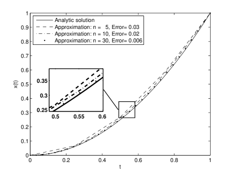
Figure 7.1: Analytic and approximate solutions of Example 50.

Let us now move to another example for which the solution is obtained by the fractional Euler–Lagrange equation.

Example 51.

Consider the following minimization problem:

$$\left\{\begin{array}[]{l}J[x(\cdot)]=\int_{0}^{1}\left({{}_{0}D_{t}^{0.5}}x(t)-\dot{x}^{2}(t)\right)dt\rightarrow\min\\ x(0)=0,~{}x(1)=1.\end{array}\right.$$ (7.12)

In this case the only way to get a solution is by use of Euler–Lagrange equations. The Lagrangian depends not only on the fractional derivative, but also on the first order derivative of the function. The Euler–Lagrange equation for this setting becomes

$$\frac{\partial L}{\partial x}+{{}_{t}D_{b}^{\alpha}}\frac{\partial L}{\partial{{}_{a}D_{t}^{\alpha}}}-\frac{d}{dt}\left(\frac{\partial L}{\partial\dot{x}}\right)=0$$

and, by direct computations, a necessary condition for $x(\cdot)$ to be a minimizer of (7.12) is

$${}_{t}D_{1}^{\alpha}1+2\ddot{x}(t)=0,~{}\mbox{or}~{}\ddot{x}(t)=\frac{1}{2\Gamma(1-\alpha)}(1-t)^{-\alpha}.$$

Subject to the given boundary conditions, the above second-order ordinary differential equation has the solution

$$x(t)=-\frac{1}{2\Gamma(3-\alpha)}(1-t)^{2-\alpha}+\left(1-\frac{1}{2\Gamma(3-\alpha)}\right)t+\frac{1}{2\Gamma(3-\alpha)}.$$ (7.13)

Discretizing problem (7.12) with the same assumptions of Example 50 ends in a linear system of the form

$$\left[\begin{array}[]{ccccccc}2&-1&0&0&\cdots&0&0\\ -1&2&-1&0&\cdots&0&0\\ 0&-1&2&-1&\cdots&0&0\\ \vdots&\vdots&\vdots&\vdots&\ddots&\vdots&\vdots\\ 0&0&0&0&\cdots&-1&2\end{array}\right]\left[\begin{array}[]{c}x_{1}\\ x_{2}\\ x_{3}\\ \vdots\\ x_{n-1}\end{array}\right]=\left[\begin{array}[]{c}b_{1}\\ b_{2}\\ b_{3}\\ \vdots\\ b_{n-1}\end{array}\right],$$ (7.14)

where

$$b_{i}=\frac{h}{2}\sum_{k=0}^{n-i-1}(-1)^{k}h^{0.5}\binom{0.5}{k},\qquad i=1,2,\cdots,n-2,$$

and

$$b_{n-1}=\frac{h}{2}\sum_{k=0}^{1}\left((-1)^{k}h^{0.5}\binom{0.5}{k}\right)+x_{n}.$$

System (7.14) is linear and can be solved for any $n$ to reach the desired accuracy. The analytic solution together with some approximated solutions are shown in Figure 7.2.

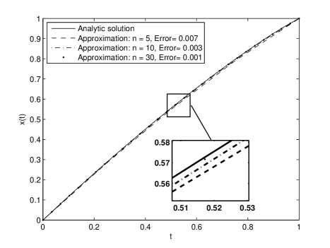
Figure 7.2: Analytic and approximate solutions of Example 51.

Both examples above end with linear systems and their solvability is simply dependant on the matrix of coefficients. Now we try our method on a more complicated problem, yet analytically solvable with an oscillating solution.

Example 52.

Let $0<\alpha<1$ and we are supposed to minimize a functional with the following Lagrangian on $[0,1]$:

$$L=\left({{}_{0}D_{t}^{0.5}}x(t)-\frac{16\Gamma(6)}{\Gamma(5.5)}t^{4.5}+\frac{20\Gamma(4)}{\Gamma(3.5)}t^{2.5}-\frac{5}{\Gamma(1.5)}t^{0.5}\right)^{4}.$$

This example has an obvious solution too. Since $L$ is positive, $\int_{0}^{1}Ldt$ subject to the boundary conditions $x(0)=0$ and $x(1)=1$ has a minimizer of the form

$$x(t)=16t^{5}-20t^{3}+5t.$$

Note that ${{}_{a}D_{t}^{\alpha}}(t-a)^{\nu}=\frac{\Gamma(\nu+1)}{\Gamma(\nu+\-\alpha)}(t-a)^{\nu-\alpha}$.

The appearance of a fourth power in the Lagrangian, results in a nonlinear system as we apply the Euler-like direct method to this problem. For $j=1,\ldots,n-1$, we have

$$\sum_{i=j}^{n}\left(\omega_{i-j}^{0.5}\right)\left(\frac{1}{h^{0.5}}\sum_{k=0}^{i}\left(\omega_{k}^{0.5}\right)x_{i-k}-\phi(t_{i})\right)^{3}=0,$$ (7.15)

where

$$\phi(t)=\frac{16\Gamma(6)}{\Gamma(5.5)}t^{4.5}+\frac{20\Gamma(4)}{\Gamma(3.5)}t^{2.5}-\frac{5}{\Gamma(1.5)}t^{0.5}.$$

System (7.15) is solved for different values of $n$ and the results are depicted in Figure 7.3.

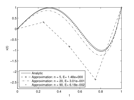
Figure 7.3: Analytic and approximate solutions of Example 52.

These examples show that an Euler-like direct method reduces a variational problem to a system of algebraic equations. When the resulting system is linear, better solutions are obtained by increasing the number of mesh points as long as the resulted matrix of coefficients is invertible. The method is very fast in this case.

The situation is completely different when the problem ends with a nonlinear system. Table 7.1 summarizes the results regarding the running time and the error.

	n	T	E
Example 1	5	$1.9668\times 10^{-4}$	0.0264
	10	$2.8297\times 10^{-4}$	0.0158
	30	$9.8318\times 10^{-4}$	0.0065
Example 2	5	$2.4053\times 10^{-4}$	0.0070
	10	$3.0209\times 10^{-4}$	0.0035
	30	$7.3457\times 10^{-4}$	0.0012
Example 3	5	0.0126	1.4787
	20	0.2012	0.3006
	90	26.355	0.0618

Table 7.1: Number of mesh points, $n$, with corresponding run time in seconds, $T$, and error, $E$ (7.9).

7.3 A discrete time method on the first variation

The fact that the first variation of a variational functional must vanish along an extremizer is the base of most effective solution schemes to solve problems of the calculus of variations. We generalize the method to variational problems involving fractional order derivatives. First order splines are used as variations, for which fractional derivatives are known. The Grünwald–Letnikov definition of fractional derivative is used, because of its intrinsic discrete nature that leads to straightforward approximations [103].

The problem under consideration is stated in the following way: find the extremizers of

$$J[x]=\int_{a}^{b}L(t,x(t),{{}_{a}D_{t}^{\alpha}}x(t))\,dt$$ (7.16)

subject to given boundary conditions $x(a)=x_{a}$ and $x(b)=x_{b}$. Here, $L:[a,b]\times\mathbb{R}^{2}\to\mathbb{R}$ is such that $\frac{\partial L}{\partial x}$ and $\frac{\partial L}{\partial{{}_{a}D_{t}^{\alpha}}x}$ exist and are continuous for all triplets $(t,x(t),{{}_{a}D_{t}^{\alpha}}x(t))$. If $x$ is a solution to the problem and $\eta:[a,b]\to\mathbb{R}$ is a variation function, i.e., $\eta(a)=\eta(b)=0$, then the first variation of $J$ at $x$, with the variation $\eta$, whatever choice of $\eta$ is taken, must vanish:

$$J^{\prime}[x,\eta]=\int_{a}^{b}\left[\frac{\partial L}{\partial x}(t,x(t),{{}_{a}D_{t}^{\alpha}}x(t))\eta(t)+\frac{\partial L}{\partial{{}_{a}D_{t}^{\alpha}}x}(t,x(t),{{}_{a}D_{t}^{\alpha}}x(t)){{}_{a}D_{t}^{\alpha}}\eta(t)\right]\,dt=0.$$ (7.17)

Using an integration by parts formula for fractional derivatives and the Dubois–Reymond lemma, Riewe [107] proved that if $x$ is an extremizer of (7.16), then

$$\frac{\partial L}{\partial x}(t,x(t),{{}_{a}D_{t}^{\alpha}}x(t))+{{}_{t}D^{\alpha}_{b}}\left(\frac{\partial L}{\partial{{}_{a}D_{t}^{\alpha}}x}\right)(t,x(t),{{}_{a}D_{t}^{\alpha}}x(t))=0$$

(see also [1]). This fractional differential equation is called an Euler–Lagrange equation. For the state of the art on the subject we refer the reader to the recent book [79]. Here, instead of solving such Euler–Lagrange equation, we apply a discretization over time and solve a system of algebraic equations. The procedure has proven to be a successful tool for classical variational problems [59, 60].

The discretization method is the following. Let $n\in\mathbb{N}$ be a fixed parameter and $h=\frac{b-a}{n}$. If we define $t_{i}=a+ih$, $x_{i}=x(t_{i})$, and $\eta_{i}=\eta(t_{i})$ for $i=0,\ldots,n$, the integral (7.17) can be approximated by the sum

$$J^{\prime}[x,\eta)]\approx h\sum_{i=1}^{n}\left[\frac{\partial L}{\partial x}(t_{i},x(t_{i}),{{}_{a}D_{t_{i}}^{\alpha}}x(t_{i}))\eta(t_{i})+\frac{\partial L}{\partial{{}_{a}D_{t}^{\alpha}}x}(t_{i},x(t_{i}),{{}_{a}D_{t_{i}}^{\alpha}}x(t_{i})){{}_{a}D_{t_{i}}^{\alpha}}\eta(t_{i})\right].$$

To compute the fractional derivative, we replace it by the sum as in (7.1), and to find an approximation for $x$ on mesh points one must solve the equation

$$\sum_{i=1}^{n} \left[\frac{\partial L}{\partial x}\left(t_{i},x_{i},\frac{1}{h^{\alpha}}\sum_{k=0}^{i}\left(\omega_{k}^{\alpha}\right)x_{i-k}\right)\eta_{i}\right.$$

$$\qquad\left.+\frac{\partial L}{\partial{{}_{a}D_{t}^{\alpha}}x}\left(t_{i},x_{i},\frac{1}{h^{\alpha}}\sum_{k=0}^{i}\left(\omega_{k}^{\alpha}\right)x_{i-k}\right)\frac{1}{h^{\alpha}}\sum_{k=0}^{i}\left(\omega_{k}^{\alpha}\right)\eta_{i-k}\right]=0.$$ (7.18)

For different choices of $\eta$, one obtains different equations. Here we use simple variations. More precisely, we use first order splines as the set of variation functions:

$$\eta_{j}(t)=\left\{\begin{array}[]{ll}\displaystyle\frac{t-t_{j-1}}{h}&\mbox{ if }t_{j-1}\leq t<t_{j},\\ \displaystyle\frac{t_{j+1}-t}{h}&\mbox{ if }t_{j}\leq t<t_{j+1},\\ 0&\mbox{ otherwise,}\end{array}\right.$$ (7.19)

for $j=1,\ldots,n-1$. We remark that conditions $\eta_{j}(a)=\eta_{j}(b)=0$ are fulfilled for all $j$, and that $\eta_{j}(t_{i})=0$ for $i\not=j$ and $\eta_{j}(t_{j})=1$. The fractional derivative of $\eta_{j}$ at any point $t_{i}$ is also computed using approximation (7.1):

$${{}_{a}D_{t_{i}}^{\alpha}}\eta_{j}(t_{i})=\left\{\begin{array}[]{ll}\displaystyle\frac{1}{h^{\alpha}}(w_{i-j}^{\alpha})&\mbox{ if }j\leq i,\\ 0&\mbox{ otherwise.}\end{array}\right.$$

Using $\eta_{j}$, $j=1,\ldots,n-1$, and equation (7.3) we establish the following system of $n-1$ algebraic equations with $n-1$ unknown variables $x_{1},\ldots,x_{n-1}$:

$$\left\{\begin{array}[]{l}\displaystyle\frac{\partial L}{\partial x}\{x_{1}\}+\frac{1}{h^{\alpha}}\sum_{i=1}^{n}\left[\frac{\partial L}{\partial{{}_{a}D_{t}^{\alpha}}x}\{x_{i}\}(w_{i-1}^{\alpha})\right]=0,\\ \displaystyle\frac{\partial L}{\partial x}\{x_{2}\}+\frac{1}{h^{\alpha}}\sum_{i=2}^{n}\left[\frac{\partial L}{\partial{{}_{a}D_{t}^{\alpha}}x}\{x_{i}\}(w_{i-2}^{\alpha})\right]=0,\\ \quad\vdots\\ \displaystyle\frac{\partial L}{\partial x}\{x_{n-1}\}+\frac{1}{h^{\alpha}}\sum_{i=n-1}^{n}\left[\frac{\partial L}{\partial{{}_{a}D_{t}^{\alpha}}x}\{x_{i}\}(w_{i-n+1}^{\alpha})\right]=0,\end{array}\right.$$ (7.20)

where we define

$$\{x_{i}\}=\left(t_{i},x_{i},\frac{1}{h^{\alpha}}\sum_{k=0}^{i}\left(\omega_{k}^{\alpha}\right)x_{i-k}\right).$$

The solution to (7.20), if exists, gives an approximation to the values of the unknown function $x$ on mesh points $t_{i}$.

We have considered so far the so called fundamental or basic problem of the fractional calculus of variations [79]. However, other types of problems can be solved applying similar techniques. Let us show how to solve numerically the isoperimetric problem, that is, when in the initial problem the set of admissible functions must satisfy some integral constraint that involves a fractional derivative. We state the fractional isoperimetric problem as follows.

Assume that the set of admissible functions are subject not only to some prescribed boundary conditions, but to some integral constraint, say

$$\int_{a}^{b}g(t,x(t),{{}_{a}D_{t}^{\alpha}}x(t))\,dt=K,$$

for a fixed $K\in\mathbb{R}$. As usual, we assume that $g:[a,b]\times\mathbb{R}^{2}\to\mathbb{R}$ is such that $\frac{\partial g}{\partial x}$ and $\frac{\partial g}{\partial{{}_{a}D_{t}^{\alpha}}x}$ exist and are continuous. The common procedure to solve this problem follows some simple steps: first we consider the auxiliary function

$$F=\lambda_{0}L(t,x(t),{{}_{a}D_{t}^{\alpha}}x(t))+\lambda g(t,x(t),{{}_{a}D_{t}^{\alpha}}x(t)),$$ (7.21)

for some constants $\lambda_{0}$ and $\lambda$ to be determined later. Next, it can be proven that $F$ satisfies the fractional Euler–Lagrange equation and that in case the extremizer does not satisfies the Euler–Lagrange associated to $g$, then we can take $\lambda_{0}=1$ (cf. [9]). In conclusion, the first variation of $F$ evaluated along an extremal must vanish, and so we obtain a system similar to (7.20), replacing $L$ by $F$. Also, from the integral constraint, we obtain another equation derived by discretization that is used to obtain $\lambda$:

$$h\sum_{i=1}^{n}g\left(t_{i},x_{i},\frac{1}{h^{\alpha}}\sum_{k=0}^{i}\left(\omega_{k}^{\alpha}\right)x_{i-k}\right)=K.$$

We show the usefulness of our approximate method with three problems of the fractional calculus of variations.

7.3.1 Basic fractional variational problems

Example 53.

Consider the following variational problem: to minimize the functional

$$J(x)=\int_{0}^{1}\left({{}_{0}D_{t}^{0.5}}x(t)-\frac{2}{\Gamma(2.5)}t^{1.5}\right)^{2}\,dt$$

subject to the boundary conditions $x(0)=0$ and $x(1)=1$. It is an easy exercise to verify that the solution is the function $x(t)=t^{2}$.

We apply our method to this problem, for the variation (7.19). The functional $J$ does not depend on $x$ and is quadratic with respect to the fractional term. Therefore, the first variation is linear. The resulting algebraic system from (7.20) is also linear and easy to solve:

$$\left\{\begin{array}[]{l}\displaystyle\sum_{i=0}^{n-1}\left(\omega_{i}^{0.5}\right)^{2}x_{1}+\sum_{i=1}^{n-1}\left(\omega_{i}^{0.5}\right)\left(\omega_{i-1}^{0.5}\right)x_{2}+\sum_{i=2}^{n-1}\left(\omega_{i}^{0.5}\right)\left(\omega_{i-2}^{0.5}\right)x_{3}\\ \quad\displaystyle+\cdots+\sum_{i=n-2}^{n-1}\left(\omega_{i}^{0.5}\right)\left(\omega_{i-(n-2)}^{0.5}\right)x_{n-1}=\frac{2h^{2}}{\Gamma(2.5)}\sum_{i=0}^{n-1}\left(\omega_{i}^{0.5}\right)(i+1)^{1.5}-\left(\omega_{0}^{0.5}\right)\left(\omega_{n-1}^{0.5}\right),\\ \displaystyle\sum_{i=0}^{n-2}\left(\omega_{i}^{0.5}\right)\left(\omega_{i+1}^{0.5}\right)x_{1}+\sum_{i=0}^{n-2}\left(\omega_{i}^{0.5}\right)^{2}x_{2}+\sum_{i=1}^{n-2}\left(\omega_{i}^{0.5}\right)\left(\omega_{i-1}^{0.5}\right)x_{3}\\ \quad\displaystyle+\cdots+\sum_{i=n-3}^{n-2}\left(\omega_{i}^{0.5}\right)\left(\omega_{i-(n-3)}^{0.5}\right)x_{n-1}=\frac{2h^{2}}{\Gamma(2.5)}\sum_{i=0}^{n-2}\left(\omega_{i}^{0.5}\right)(i+2)^{1.5}-\left(\omega_{0}^{0.5}\right)\left(\omega_{n-2}^{0.5}\right),\\ \qquad\vdots\\ \displaystyle\sum_{i=0}^{1}\left(\omega_{i}^{0.5}\right)\left(\omega_{i+n-2}^{0.5}\right)x_{1}+\sum_{i=0}^{1}\left(\omega_{i}^{0.5}\right)\left(\omega_{i+n-3}^{0.5}\right)x_{2}+\sum_{i=0}^{1}\left(\omega_{i}^{0.5}\right)\left(\omega_{i+n-4}^{0.5}\right)x_{3}\\ \quad\displaystyle+\cdots+\sum_{i=0}^{1}\left(\omega_{i}^{0.5}\right)^{2}x_{n-1}=\frac{2h^{2}}{\Gamma(2.5)}\sum_{i=0}^{1}\left(\omega_{i}^{0.5}\right)(i+n-1)^{1.5}-\left(\omega_{0}^{0.5}\right)\left(\omega_{1}^{0.5}\right).\end{array}\right.$$

The exact solution together with three numerical approximations, with different discretization step sizes, are depicted in Figure 7.4.

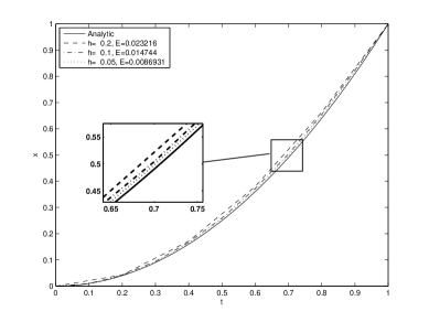
Figure 7.4: Exact solution versus numerical approximations to Example 53.

Example 54.

Find the minimizer of the functional

$$J(x)=\int_{0}^{1}\left({{}_{0}D_{t}^{0.5}}x(t)-\frac{16\Gamma(6)}{\Gamma(5.5)}t^{4.5}+\frac{20\Gamma(4)}{\Gamma(3.5)}t^{2.5}-\frac{5}{\Gamma(1.5)}t^{0.5}\right)^{4}\,dt$$

subject to $x(0)=0$ and $x(1)=1$. The minimum value of this functional is zero and the minimizer is

$$x(t)=16t^{5}-20t^{3}+5t.$$

Discretizing the first variation as discussed above, leads to a nonlinear system of algebraic equation. Its solution, using different step sizes, is depicted in Figure 7.5.

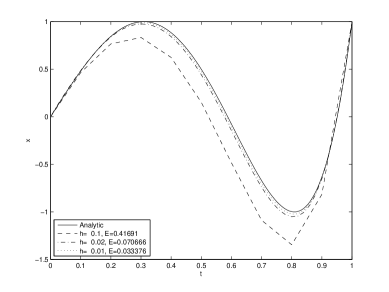
Figure 7.5: Exact solution versus numerical approximations to Example 54.

7.3.2 An isoperimetric fractional variational problem

Example 55.

Let us search the minimizer of

$$J(x)=\int_{0}^{1}\left(t^{4}+\left({{}_{0}D_{t}^{0.5}}x(t)\right)^{2}\right)\,dt$$

subject to the boundary conditions

$$x(0)=0\quad\mbox{and}\quad x(1)=\frac{16}{15\Gamma(0.5)}$$

and the integral constraint

$$\int_{0}^{1}t^{2}\,{{}_{0}D_{t}^{0.5}}x(t)\,dt=\frac{1}{5}.$$

In [13] it is shown that the solution to this problem is the function

$$x(t)=\frac{16t^{2.5}}{15\Gamma(0.5)}.$$

Because $x$ does not satisfy the fractional Euler–Lagrange equation associated to the integral constraint, one can take $\lambda_{0}=1$ and the auxiliary function (7.21) is $F=t^{4}+\left({{}_{0}D_{t}^{0.5}}x(t)\right)^{2}+\lambda\,t^{2}\,{{}_{0}D_{t}^{0.5}}x(t)$. Now we calculate the first variation of $\int_{0}^{1}Fdt$. An extra unknown, $\lambda$, is present in the new setting, that is obtained by discretizing the integral constraint, as explained in Section 7.3. The solutions to the resulting algebraic system, with different step sizes, are given in Figure 7.6.

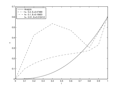
Figure 7.6: Exact versus numerical approximations to the isoperimetric problem of Example 55.

Chapter 8 Indirect methods

As in the classical case, indirect methods in fractional sense provide necessary conditions of optimality using the first variation. Fractional Euler–Lagrange equations are now a well-known and well-studied subject in fractional calculus. For a simple problem of the form (3.1), following [1], a necessary condition implies that the solution must satisfy a fractional boundary value differential equation.

Let $x(\cdot)$ have a continuous left Riemann–Liouville derivative of order $\alpha$ and $J[x]$ be a functional of the form

$$J[x(\cdot)]=\int_{a}^{b}L(t,x(t),{{}_{a}D_{t}^{\alpha}}x(t))dt$$ (8.1)

subject to the boundary conditions $x(a)=x_{a}$ and $x(b)=x_{b}$. Recall that

$$\left\{\begin{array}[]{l}\frac{\partial L}{\partial x}+{{}_{t}D_{b}^{\alpha}}\frac{\partial L}{\partial~{}{{}_{a}D_{t}^{\alpha}}x}=0\\ x(a)=x_{a},\quad x(b)=x_{b}\end{array}\right.$$ (8.2)

is the fractional Euler–Lagrange equation and is a necessary optimality condition.

Many variants of (8.2) can be found in the literature. Different types of fractional terms have been embedded in the Lagrangian and appropriate versions of Euler–Lagrange equations have been derived using proper integration by parts formulas. See [8, 12, 21, 77, 87] for details.

For fractional optimal control problems, a so called Hamiltonian system is constructed using Lagrange multipliers. For example, cf. [25]. Assume that we are required to minimize a functional of the form

$$J[x(\cdot),u(\cdot)]=\int_{a}^{b}L(t,x(t),u(t))dt$$

such that $x(a)=x_{a}$, $x(b)=x_{b}$ and ${{}_{a}D_{t}^{\alpha}}x(t)=f(t,x(t),u(t))$. Similar to the classical methods, one can introduce a Hamiltonian

$$H=L(t,x(t),u(t))+\lambda(t)f(t,x(t),u(t)),$$

where $\lambda(t)$ is considered as a Lagrange multiplier. In this case we define the augmented functional as

$$J[x(\cdot),u(\cdot)]=\int_{a}^{b}[H(t,x(t),u(t),\lambda(t))-\lambda(t){{}_{a}D_{t}^{\alpha}}x(t)]dt.$$

Optimizing the latter functional results into the following necessary optimality conditions:

$$\left\{\begin{array}[]{l}{{}_{a}D_{t}^{\alpha}}x(t)=\displaystyle\frac{\partial H}{\partial\lambda}\\[8.0pt] {{}_{t}D_{b}^{\alpha}}\lambda(t)=\displaystyle\frac{\partial H}{\partial x}\end{array}\right.,\qquad\frac{\partial H}{\partial u}=0.$$ (8.3)

Together with the prescribed boundary conditions, this makes a two point fractional boundary value problem.

These arguments reveal that, like in the classical case, fractional variational problems end with fractional boundary value problems. To reach an optimal solution, one needs to deal with a fractional differential equation or a system of fractional differential equations. There are a few attempts in the literature to present analytic solutions to fractional variational problems. Simple problems have been treated in [16]; some other examples are presented in [20].

Many solution methods, theoretical and numerical, furnish the classical theory of differential equations; nevertheless, solving a fractional differential equation is a rather tough task [38]. To benefit from those methods, especially all solvers that are available to solve an integer-order differential equation numerically, we can either approximate a fractional variational problem by an equivalent integer-order one or approximate the necessary optimality conditions (8.2) and (8.3). The rest of this section discusses two types of approximations that are used to transform a fractional problem to one in which only integer-order derivatives are present, i.e., we approximate the original problem by substituting a fractional term by its corresponding expansion formulas. This is mainly done by case studies on certain examples. The examples are chosen so that either they have a trivial solution or it is possible to get an analytic solution using the fractional Euler–Lagrange equations [98].

By substituting the approximations (5.4) or (5.10) for the fractional derivative in (8.1), the problem is transformed to

$$J[x(\cdot)] \approx \int_{a}^{b}L\left(t,x(t),\sum_{k=0}^{N}\frac{(-1)^{k-1}\alpha x^{(k)}(t)}{k!(k-\alpha)\Gamma(1-\alpha)}(t-a)^{k-\alpha}\right)dt$$

$$= \int_{a}^{b}L^{\prime}\left(t,x(t),\dot{x}(t),\ldots,x^{(N)}(t)\right)dt$$

or

$$J[x(\cdot)] \approx \int_{a}^{b}L\left(t,x(t),\frac{Ax(t)}{(t-a)^{\alpha}}+\frac{B\dot{x}(t)}{(t-a)^{\alpha-1}}-\sum_{p=2}^{N}\frac{C(\alpha,p)V_{p}(t)}{(t-a)^{p+\alpha-1}}\right)dt$$

$$= \int_{a}^{b}L^{\prime}\left(t,x(t),\dot{x}(t),V_{2}(t),\ldots,V_{N}(t)\right)dt$$

with

$$\left\{\begin{array}[]{l}\dot{V}_{p}(t)=(1-p)(t-a)^{p-2}x(t)\\ V_{p}(a)=0,\qquad p=2,3,\ldots\end{array}\right.$$

The former problem is a classical variational problem containing higher order derivatives. The latter is a multi-state problem, subject to an ordinary differential equation constraint. Together with the boundary conditions, both above problems belong to classes of well studied variational problems.

To accomplish a detailed study, as test problems, we consider here Example 51,

$$\left\{\begin{array}[]{l}J[x(\cdot)]=\int_{0}^{1}\left({{}_{0}D_{t}^{0.5}}x(t)-\dot{x}^{2}(t)\right)dt\rightarrow\min\\ x(0)=0,~{}x(1)=1,\end{array}\right.$$ (8.4)

and the following example.

Example 56.

Given $\alpha\in(0,1)$, consider the functional

$$J[x(\cdot)]=\int_{0}^{1}({{}_{a}D_{t}^{\alpha}}x(t)-1)^{2}dt$$ (8.5)

to be minimized subject to the boundary conditions $x(0)=0$ and $x(1)=\frac{1}{\Gamma(\alpha+1)}$. Since the integrand in (8.5) is non-negative, the functional attains its minimum when ${{}_{a}D_{t}^{\alpha}}x(t)=1$, i.e., for $x(t)=\frac{t^{\alpha}}{\Gamma(\alpha+1)}$.

We illustrate the use of the two different expansions separately.

8.1 Expansion to integer orders

Using approximation (5.4) for the fractional derivative in (8.4), we get the approximated problem

$$\tilde{J}[x(\cdot)]=\int_{0}^{1}\left[\sum_{n=0}^{N}C(n,\alpha)t^{n-\alpha}x^{(n)}(t)-\dot{x}^{2}(t)\right]dt\longrightarrow\min$$ (8.6)

$$x(0)=0,\quad x(1)=1,$$

which is a classical higher-order problem of the calculus of variations that depends on derivatives up to order $N$. The corresponding necessary optimality condition is a well-known result.

Theorem 57 (cf., e.g., [71]).

Suppose that $x(\cdot)\in C^{2N}[a,b]$ minimizes

$$\int_{a}^{b}L(t,x(t),x^{(1)}(t),x^{(2)}(t),\ldots,x^{(N)}(t))dt$$

with given boundary conditions

$$x(a)=a_{0}, x(b)=b_{0},$$

$$x^{(1)}(a)=a_{1}, x^{(1)}(b)=b_{1},$$

$$\vdots$$

$$x^{(N-1)}(a)=a_{N-1}, x^{(N-1)}(b)=b_{N-1}.$$

Then $x(\cdot)$ satisfies the Euler–Lagrange equation

$$\frac{\partial L}{\partial x}-\frac{d}{dt}\left(\frac{\partial L}{\partial x^{(1)}}\right)+\frac{d^{2}}{dt^{2}}\left(\frac{\partial L}{\partial x^{(2)}}\right)-\cdots+(-1)^{N}\frac{d^{N}}{dt^{N}}\left(\frac{\partial L}{\partial x^{(N)}}\right)=0.$$ (8.7)

In general (8.7) is an ODE of order $2N$, depending on the order $N$ of the approximation we choose, and the method leaves $2N-2$ parameters unknown. In our example, however, the Lagrangian in (8.6) is linear with respect to all derivatives of order higher than two. The resulting Euler–Lagrange equation is the second-order ODE

$$\sum_{n=0}^{N}(-1)^{n}C(n,\alpha)\frac{d^{n}}{dt^{n}}(t^{n-\alpha})-\frac{d}{dt}\left[-2\dot{x}(t)\right]=0,$$

that has the solution

$$x(t)=M_{1}(\alpha,N)t^{2-\alpha}+M_{2}(\alpha,N)t,$$

where

$$M_{1}(\alpha,N) = -\frac{1}{2\Gamma(3-\alpha)}\left[\sum_{n=0}^{N}(-1)^{n}\Gamma(n+1-\alpha)C(n,\alpha)\right],$$

$$M_{2}(\alpha,N) = \left[1+\frac{1}{2\Gamma(3-\alpha)}\sum_{n=0}^{N}(-1)^{n}\Gamma(n+1-\alpha)C(n,\alpha)\right].$$

Figure 8.1 shows the analytic solution together with several approximations. It reveals that by increasing $N$, approximate solutions do not converge to the analytic one. The reason is the fact that the solution (7.13) to Example 51 is not an analytic function. We conclude that (5.4) may not be a good choice to approximate fractional variational problems. In contrast, as we shall see, the approximation (5.10) leads to good results.

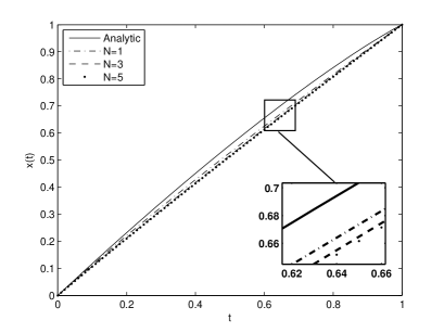
Figure 8.1: Analytic versus approximate solutions to Example 51 using approximation (5.4) with $\alpha=0.5$.

To solve Example 51 using (5.4) as an approximation for the fractional derivative, the problem becomes

$$\tilde{J}[x(\cdot)]=\int_{0}^{1}\left(\sum_{n=0}^{N}C(n,\alpha)t^{n-\alpha}x^{(n)}(t)-1\right)^{2}dt\longrightarrow\min$$

$$x(0)=0,\quad x(1)=\frac{1}{\Gamma(\alpha+1)}.$$

The Euler–Lagrange equation (8.7) gives a $2N$ order ODE. For $N\geq 2$ this approach is inappropriate since the two given boundary conditions $x(0)=0$ and $x(1)=\frac{1}{\Gamma(\alpha+1)}$ are not enough to determine the $2N$ constants of integration.

8.2 Expansion through the moments of a function

If we use (5.10) to approximate the optimization problem (8.4), with $A=A(\alpha,N)$, $B=B(\alpha,N)$ and $C_{p}=C(\alpha,p)$, we have

$$\begin{split}\tilde{J}[x(\cdot)]&=\int_{0}^{1}\left[At^{-\alpha}x(t)+Bt^{1-\alpha}\dot{x}(t)-\sum_{p=2}^{N}C_{p}t^{1-p-\alpha}V_{p}(t)-\dot{x}^{2}(t)\right]dt\longrightarrow\min\\ \dot{V}_{p}(t)&=(1-p)t^{p-2}x(t),\quad p=2,3,\ldots,N,\\ V_{p}(0)&=0,\quad p=2,3,\ldots,N,\\ x(0)&=0,\quad x(1)=1.\end{split}$$ (8.8)

Problem (8.8) is constrained with a set of ordinary differential equations and is natural to look to it as an optimal control problem [94]. For that, we introduce the control variable $u(t)=\dot{x}(t)$. Then, using the Lagrange multipliers $\lambda_{1},\lambda_{2},\ldots,\lambda_{N}$, and the Hamiltonian system, one can reduce (8.8) to the study of the two point boundary value problem

$$\left\{\begin{array}[]{rl}\dot{x}(t)&=\frac{1}{2}Bt^{1-\alpha}-\frac{1}{2}\lambda_{1}(t),\\ \dot{V}_{p}(t)&=(1-p)t^{p-2}x(t),\quad p=2,3,\ldots,N,\\ \dot{\lambda}_{1}(t)&=At^{-\alpha}-\sum_{p=2}^{N}(1-p)t^{p-2}\lambda_{p}(t),\\ \dot{\lambda}_{p}(t)&=-C_{p}t^{(1-p-\alpha)},\quad p=2,3,\ldots,N,\\ \end{array}\right.$$ (8.9)

with boundary conditions

$$\left\{\begin{array}[]{l}x(0)=0,\\ V_{p}(0)=0,\quad p=2,3,\ldots,N,\end{array}\right.\qquad\left\{\begin{array}[]{l}x(1)=1,\\ \lambda_{p}(1)=0,\quad p=2,3,\ldots,N,\end{array}\right.$$

where $x(0)=0$ and $x(1)=1$ are given. We have $V_{p}(0)=0$, $p=2,3,\ldots,N$, due to (5.9) and $\lambda_{p}(1)=0$, $p=2,3,\ldots,N$, because $V_{p}$ is free at final time for $p=2,3,\ldots,N$ [94]. In general, the Hamiltonian system is a nonlinear, hard to solve, two point boundary value problem that needs special numerical methods. In this case, however, (8.9) is a non-coupled system of ordinary differential equations and is easily solved to give

$$x(t)=M(\alpha,N)t^{2-\alpha}-\sum_{p=2}^{N}\frac{C(\alpha,p)}{2p(2-p-\alpha)}t^{p}+\left[1-M(\alpha,N)+\sum_{p=2}^{N}\frac{C(\alpha,p)}{2p(2-p-\alpha)}\right]t,$$

where

$$M(\alpha,N)=\frac{1}{2(2-\alpha)}\left[B(\alpha,N)-\frac{A(\alpha,N)}{1-\alpha}-\sum_{p=2}^{N}\frac{C(\alpha,p)(1-p)}{(1-\alpha)(2-p-\alpha)}\right].$$

Figure 8.2 shows the graph of $x(\cdot)$ for different values of $N$.

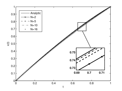
Figure 8.2: Analytic versus approximate solutions to Example 51 using approximation (5.10) with $\alpha=0.5$.

Let us now approximate Example 56 using (5.10). The resulting minimization problem has the following form:

$$\tilde{J}[x(\cdot)]=\int_{0}^{1}\left[At^{-\alpha}x(t)+Bt^{1-\alpha}\dot{x}(t)-\sum_{p=2}^{N}C_{p}t^{1-p-\alpha}V_{p}(t)-1\right]^{2}dt\longrightarrow\min$$ (8.10)

$$\dot{V}_{p}(t)=(1-p)t^{p-2}x(t),\quad p=2,3,\ldots,N,$$

$$V_{p}(0)=0,\quad p=2,3,\ldots,N,$$

$$x(0)=0,\quad x(1)=\frac{1}{\Gamma(\alpha+1)}.$$

Following the classical optimal control approach of Pontryagin [94], this time with

$$u(t)=At^{-\alpha}x(t)+Bt^{1-\alpha}\dot{x}(t)-\sum_{p=2}^{N}C_{p}t^{1-p-\alpha}V_{p}(t),$$

we conclude that the solution to (8.10) satisfies the system of differential equations

$$\left\{\begin{array}[]{rl}\dot{x}(t)&=-AB^{-1}t^{-1}x(t)+\sum_{p=2}^{N}B^{-1}C_{p}t^{-p}V_{p}(t)+\frac{1}{2}B^{-2}t^{2\alpha-2}\lambda_{1}(t)+B^{-1}t^{\alpha-1},\\ \dot{V}_{p}(t)&=(1-p)t^{p-2}x(t),\quad p=2,3,\ldots,N,\\ \dot{\lambda}_{1}(t)&=AB^{-1}t^{-1}\lambda_{1}-\sum_{p=2}^{N}(1-p)t^{p-2}\lambda_{p}(t),\\ \dot{\lambda}_{p}(t)&=-B^{-1}C_{p}t^{-p}\lambda_{1},\quad p=2,3,\ldots,N,\\ \end{array}\right.$$ (8.11)

where $A=A(\alpha,N)$, $B=B(\alpha,N)$ and $C_{p}=C(\alpha,p)$ are defined according to Section 5.1.2, subject to the boundary conditions

$$\left\{\begin{array}[]{l}x(0)=0,\\ V_{p}(0)=0,\quad p=2,3,\ldots,N,\end{array}\right.\qquad\left\{\begin{array}[]{l}x(1)=\displaystyle\frac{1}{\Gamma(\alpha+1)},\\ \lambda_{p}(1)=0,\quad p=2,3,\ldots,N.\end{array}\right.$$ (8.12)

The solution to system (8.11)–(8.12), with $N=2$, is shown in Figure 8.3.

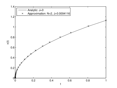
Figure 8.3: Analytic versus approximate solution to Example 56 using approximation (5.10) with $\alpha=0.5$.

Chapter 9 Fractional optimal control with free end-points

This chapter is devoted to fractional order optimal control problems in which the dynamic control system involves integer and fractional order derivatives and the terminal time is free. Necessary conditions for a state/control/terminal-time triplet to be optimal are obtained. Situations with constraints present at the end time are also considered. Under appropriate assumptions, it is shown that the obtained necessary optimality conditions become sufficient. Numerical methods to solve the problems are presented, and some computational simulations are discussed in detail [102].

9.1 Necessary optimality conditions

Let $\alpha\in(0,1)$, $a\in\mathbb{R}$, $L$ and $f$ be two differentiable functions with domain $[a,+\infty)\times\mathbb{R}^{2}$, and $\phi:[a,+\infty)\times\mathbb{R}\rightarrow\mathbb{R}$ be a differentiable function. The fundamental problem is stated in the following way:

$$J[x,u,T]=\int_{a}^{T}L(t,x(t),u(t))\,dt+\phi(T,x(T))\longrightarrow\min$$ (9.1)

subject to the control system

$$M\dot{x}(t)+N\;{{}^{C}_{a}D_{t}^{\alpha}}x(t)=f(t,x(t),u(t)),$$ (9.2)

and the initial boundary condition

$$x(a)=x_{a},$$ (9.3)

with $(M,N)\not=(0,0)$ and $x_{a}$ a fixed real number. Our goal is to generalize previous works on fractional optimal control problems by considering the end time, $T$, free and the dynamic control system (9.2) involving integer and fractional order derivatives. For convenience, we consider the one-dimensional case. However, using similar techniques, the results can be easily extended to problems with multiple states and multiple controls. Later we consider the cases $T$ and/or $x(T)$ fixed. Here, $T$ is a variable number with $a<T<\infty$. Thus, we are interested not only on the optimal trajectory $x$ and optimal control function $u$, but also on the corresponding time $T$ for which the functional $J$ attains its minimum value. We assume that the state variable $x$ is differentiable and that the control $u$ is piecewise continuous. When $N=0$ we obtain a classical optimal control problem; the case $M=0$ with fixed $T$ has already been studied for different types of fractional order derivatives (see, e.g., [2, 5, 7, 54, 53, 119, 120]). In [63] a special type of the proposed problem is also studied for fixed $T$.

Remark 58.

In this chapter the terminal time $T$ is a free decision variable and, a priori, no constraints are imposed. For future research, one may wish to consider a class of fractional optimal control problems in which the terminal time is governed by a stopping condition. Such problems were recently investigated, within the classical (integer-order) framework, in [73, 74].

9.1.1 Fractional necessary conditions

To deduce necessary optimality conditions that an optimal triplet $(x,u,T)$ must satisfy, we use a Lagrange multiplier to adjoin the dynamic constraint (9.2) to the performance functional (9.1). To start, we define the Hamiltonian function $H$ by

$$H(t,x,u,\lambda)=L(t,x,u)+\lambda f(t,x,u),$$ (9.4)

where $\lambda$ is a Lagrange multiplier, so that we can rewrite the initial problem as minimizing

$$\mathcal{J}[x,u,T,\lambda]=\int_{a}^{T}\left[H(t,x,u,\lambda)-\lambda(t)[M\dot{x}(t)+N\;{{}^{C}_{a}D_{t}^{\alpha}}x(t)]\right]\,dt+\phi(T,x(T)).$$

Next, we consider variations of the form

$$x+\delta x,\quad u+\delta u,\quad T+\delta T,\quad\lambda+\delta\lambda,$$

with $\delta x(a)=0$ by the imposed boundary condition (9.3). Using the well-known fact that the first variation of $\mathcal{J}$ must vanish when evaluated along a minimizer, we get

$$0=\int_{a}^{T}\Biggl{(}\frac{\partial H}{\partial x}\delta x+\frac{\partial H}{\partial u}\delta u+\frac{\partial H}{\partial\lambda}\delta\lambda-\delta\lambda\left(M\dot{x}(t)+N\;{{}^{C}_{a}D_{t}^{\alpha}}x(t)\right)\\ -\lambda(t)\left(M\dot{\delta x}(t)+N\;{{}^{C}_{a}D_{t}^{\alpha}}\delta x(t)\right)\Biggr{)}dt+\delta T\bigl{[}H(t,x,u,\lambda)\\ -\lambda(t)\left(M\dot{x}(t)+N\;{{}^{C}_{a}D_{t}^{\alpha}}x(t)\right)\bigr{]}_{t=T}+\frac{\partial\phi}{\partial t}(T,x(T))\delta T+\frac{\partial\phi}{\partial x}(T,x(T))\left(\dot{x}(T)\delta T+\delta x(T)\right)$$

with the partial derivatives of $H$ evaluated at $(t,x(t),u(t),\lambda(t))$. Integration by parts gives the relations

$$\int_{a}^{T}\lambda(t)\dot{\delta x}(t)\,dt=-\int_{a}^{T}\delta x(t)\dot{\lambda}(t)\,dt+\delta x(T)\lambda(T)$$

and

$$\int_{a}^{T}\lambda(t){{}^{C}_{a}D_{t}^{\alpha}}\delta x(t)\,dt=\int_{a}^{T}\delta x(t)\,{{}_{t}D_{T}^{\alpha}}\lambda(t)\,dt+\delta x(T)[{{}_{t}I_{T}^{1-\alpha}}\lambda(t)]_{t=T}.$$

Thus, we deduce the following formula:

$$\int_{a}^{T}\left[\delta x\left(\frac{\partial H}{\partial x}+M\dot{\lambda}-N\;{{}_{t}D_{T}^{\alpha}}\lambda\right)+\delta u\frac{\partial H}{\partial u}+\delta\lambda\left(\frac{\partial H}{\partial\lambda}-M\dot{x}-N\;{{}^{C}_{a}D_{t}^{\alpha}}x\right)\right]dt\\ -\delta x(T)\left[M\lambda+N\;{{}_{t}I_{T}^{1-\alpha}}\lambda-\frac{\partial\phi}{\partial x}(t,x)\right]_{t=T}\\ +\delta T\left[H(t,x,u,\lambda)-\lambda[M\dot{x}+N\;{{}^{C}_{a}D_{t}^{\alpha}}x]+\frac{\partial\phi}{\partial t}(t,x)+\frac{\partial\phi}{\partial x}(t,x)\dot{x}\right]_{t=T}=0.$$

Now, define the new variable

$$\delta x_{T}=[x+\delta x](T+\delta T)-x(T).$$

Because $\delta\dot{x}(T)$ is arbitrary, in particular one can consider variation functions for which $\delta\dot{x}(T)=0$. By Taylor’s theorem,

$$[x+\delta x](T+\delta T)-[x+\delta x](T)=\dot{x}(T)\delta T+O(\delta T^{2}),$$

where $\displaystyle\lim_{\zeta\to 0}\frac{O(\zeta)}{\zeta}$ is finite, and so $\delta x(T)=\delta x_{T}-\dot{x}(T)\delta T+O(\delta T^{2})$. In conclusion, we arrive at the expression

$$\delta T\left[H(t,x,u,\lambda)-N\lambda(t){{}^{C}_{a}D_{t}^{\alpha}}x(t)+N\dot{x}(t){{}_{t}I_{T}^{1-\alpha}}\lambda(t)+\frac{\partial\phi}{\partial t}(t,x(t))\right]_{t=T}\\ +\int_{a}^{T}\left[\delta x\left(\frac{\partial H}{\partial x}+M\dot{\lambda}(t)-N\;{{}_{t}D_{T}^{\alpha}}\lambda(t)\right)+\delta\lambda\left(\frac{\partial H}{\partial\lambda}-M\dot{x}(t)-N\;{{}^{C}_{a}D_{t}^{\alpha}}x(t)\right)\right.\\ \left.+\delta u\frac{\partial H}{\partial u}\right]dt-\delta x_{T}\left[M\lambda(t)+N\;{{}_{t}I_{T}^{1-\alpha}}\lambda(t)-\frac{\partial\phi}{\partial x}(t,x(t))\right]_{t=T}+O(\delta T^{2})=0.$$

Since the variation functions were chosen arbitrarily, the following theorem is proven.

Theorem 59.

If $(x,u,T)$ is a minimizer of (9.1) under the dynamic constraint (9.2) and the boundary condition (9.3), then there exists a function $\lambda$ for which the triplet $(x,u,\lambda)$ satisfies:

• the Hamiltonian system

  $$\begin{cases}M\dot{\lambda}(t)-N\;{{}_{t}D_{T}^{\alpha}}\lambda(t)=-\displaystyle\frac{\partial H}{\partial x}(t,x(t),u(t),\lambda(t))\\[8.0pt] M\dot{x}(t)+N\;{{}^{C}_{a}D_{t}^{\alpha}}x(t)=\displaystyle\frac{\partial H}{\partial\lambda}(t,x(t),u(t),\lambda(t))\end{cases}$$ (9.5)

  for all $t\in[a,T]$;

• the stationary condition

  $$\frac{\partial H}{\partial u}(t,x(t),u(t),\lambda(t))=0$$ (9.6)

  for all $t\in[a,T]$;

• and the transversality conditions

  $$\begin{gathered}\left[H(t,x(t),u(t),\lambda(t))-N\lambda(t){{}^{C}_{a}D_{t}^{\alpha}}x(t)+N\dot{x}(t){{}_{t}I_{T}^{1-\alpha}}\lambda(t)+\frac{\partial\phi}{\partial t}(t,x(t))\right]_{t=T}=0,\\ \left[M\lambda(t)+N\;{{}_{t}I_{T}^{1-\alpha}}\lambda(t)-\frac{\partial\phi}{\partial x}(t,x(t))\right]_{t=T}=0;\end{gathered}$$ (9.7)

where the Hamiltonian $H$ is defined by (9.4).

Remark 60.

In standard optimal control, a free terminal time problem can be converted into a fixed final time problem by using the well-known transformation $s=t/T$ (see Example 70). This transformation does not work in the fractional setting. Indeed, in standard optimal control, translating the problem from time $t$ to a new time variable $s$ is straightforward: the chain rule gives $\frac{dx}{ds}=\frac{dx}{dt}\frac{dt}{ds}$. For Caputo or Riemann–Liouville fractional derivatives, the chain rule has no practical use and such conversion is not possible.

Some interesting special cases are obtained when restrictions are imposed on the end time $T$ or on $x(T)$.

Corollary 61.

Let $(x,u)$ be a minimizer of (9.1) under the dynamic constraint (9.2) and the boundary condition (9.3).

1. If $T$ is fixed and $x(T)$ is free, then Theorem 59 holds with the transversality conditions (9.7) replaced by

   $$\left[M\lambda(t)+N\;{{}_{t}I_{T}^{1-\alpha}}\lambda(t)-\frac{\partial\phi}{\partial x}(t,x(t))\right]_{t=T}=0.$$

2. If $x(T)$ is fixed and $T$ is free, then Theorem 59 holds with the transversality conditions (9.7) replaced by

   $$\left[H(t,x(t),u(t),\lambda(t))-N\lambda(t){{}^{C}_{a}D_{t}^{\alpha}}x(t)+N\dot{x}(t){{}_{t}I_{T}^{1-\alpha}}\lambda(t)+\frac{\partial\phi}{\partial t}(t,x(t))\right]_{t=T}=0.$$

3. If $T$ and $x(T)$ are both fixed, then Theorem 59 holds with no transversality conditions.

4. If the terminal point $x(T)$ belongs to a fixed curve, i.e., $x(T)=\gamma(T)$ for some differentiable curve $\gamma$, then Theorem 59 holds with the transversality conditions (9.7) replaced by

   $$\Biggl{[}H(t,x(t),u(t),\lambda(t))-N\lambda(t){{}^{C}_{a}D_{t}^{\alpha}}x(t)+N\dot{x}(t){{}_{t}I_{T}^{1-\alpha}}\lambda(t)+\frac{\partial\phi}{\partial t}(t,x(t))\\ -\dot{\gamma}(t)\left(M\lambda(t)+N\;{{}_{t}I_{T}^{1-\alpha}}\lambda(t)-\frac{\partial\phi}{\partial x}(t,x(t))\right)\Biggr{]}_{t=T}=0.$$

5. If $T$ is fixed and $x(T)\geq K$ for some fixed $K\in\mathbb{R}$, then Theorem 59 holds with the transversality conditions (9.7) replaced by

   $$\left[M\lambda(t)+N\;{{}_{t}I_{T}^{1-\alpha}}\lambda(t)-\frac{\partial\phi}{\partial x}(t,x(t))\right]_{t=T}\leq 0,$$

   $$(x(T)-K)\left[M\lambda(t)+N\;{{}_{t}I_{T}^{1-\alpha}}\lambda(t)-\frac{\partial\phi}{\partial x}(t,x(t))\right]_{t=T}=0.$$

6. If $x(T)$ is fixed and $T\leq K$ for some fixed $K\in\mathbb{R}$, then Theorem 59 holds with the transversality conditions (9.7) replaced by

   $$\left[H(t,x(t),u(t),\lambda(t))-N\lambda(t){{}^{C}_{a}D_{t}^{\alpha}}x(t)+N\dot{x}(t){{}_{t}I_{T}^{1-\alpha}}\lambda(t)+\frac{\partial\phi}{\partial t}(t,x(t))\right]_{t=T}\geq 0,$$

   $$\left[H(t,x(t),u(t),\lambda(t))-N\lambda(t){{}^{C}_{a}D_{t}^{\alpha}}x(t)+N\dot{x}(t){{}_{t}I_{T}^{1-\alpha}}\lambda(t)+\frac{\partial\phi}{\partial t}(t,x(t))\right]_{t=T}\\ \times(T-K)=0.$$

Proof.

The first three conditions are obvious. The fourth follows from

$$\delta x_{T}=\gamma(T+\delta T)-\gamma(T)=\dot{\gamma}(T)\delta T+O(\delta T^{2}).$$

To prove 5, observe that we have two possible cases. If $x(T)>K$, then $\delta x_{T}$ may take negative and positive values, and so we get

$$\left[M\lambda(t)+N\;{{}_{t}I_{T}^{1-\alpha}}\lambda(t)-\frac{\partial\phi}{\partial x}(t,x(t))\right]_{t=T}=0.$$

On the other hand, if $x(T)=K$, then $\delta x_{T}\geq 0$ and so by the KKT theorem

$$\left[M\lambda(t)+N\;{{}_{t}I_{T}^{1-\alpha}}\lambda(t)-\frac{\partial\phi}{\partial x}(t,x(t))\right]_{t=T}\leq 0.$$

The proof of the last condition is similar. ∎

Case 1 of Corollary 61 was proven in [54] for $(M,N)=(0,1)$ and $\phi\equiv 0$. Moreover, if $\alpha=1$, then we obtain the classical necessary optimality conditions for the standard optimal control problem (see, e.g., [36]):

• the Hamiltonian system

  $$\begin{cases}\dot{x}(t)=\displaystyle\frac{\partial H}{\partial\lambda}(t,x(t),u(t),\lambda(t)),\\[8.0pt] \dot{\lambda}(t)=-\displaystyle\frac{\partial H}{\partial x}(t,x(t),u(t),\lambda(t)),\end{cases}$$

• the stationary condition

  $$\frac{\partial H}{\partial u}(t,x(t),u(t),\lambda(t))=0,$$

• the transversality condition $\lambda(T)=0$.

9.1.2 Approximated integer-order necessary optimality conditions

Using approximation (5.10), and the relation between Caputo and Riemann–Liouville derivatives, up to order $K$, we can transform the original problem (9.1)–(9.3) into the following classical problem:

$$\tilde{J}[x,u,T]=\int_{a}^{T}L(t,x(t),u(t))\,dt+\phi(T,x(T))\longrightarrow\min$$

subject to

$$\begin{cases}\dot{x}(t)=\displaystyle\frac{f(t,x(t),u(t))-NA(t-a)^{-\alpha}x(t)+\sum_{p=2}^{K}NC_{p}(t-a)^{1-p-\alpha}V_{p}(t)-\frac{x(a)(t-a)^{-\alpha}}{\Gamma(1-\alpha)}}{M+NB(t-a)^{1-\alpha}},\\[7.11317pt] \dot{V}_{p}(t)=(1-p)(t-a)^{p-2}x(t),\quad p=2,\ldots,K,\end{cases}$$

and

$$\begin{cases}x(a)=x_{a},\\ V_{p}(a)=0,\quad p=2,\ldots,K,\end{cases}$$ (9.8)

where $A=A(\alpha,K)$, $B=B(\alpha,K)$ and $C_{p}=C(\alpha,p)$ are the coefficients in the approximation (5.10). Now that we are dealing with an integer-order problem, so we can follow a classical procedure (see, e.g., [68]), by defining the Hamiltonian $H$ by

$$\begin{split}H=L(t,x,u)&+\frac{\lambda_{1}\left(f(t,x,u)-NA(t-a)^{-\alpha}x+\sum_{p=2}^{K}NC_{p}(t-a)^{1-p-\alpha}V_{p}-\frac{x(a)(t-a)^{-\alpha}}{\Gamma(1-\alpha)}\right)}{M+NB(t-a)^{1-\alpha}}\\ &+\sum_{p=2}^{K}\lambda_{p}(1-p)(t-a)^{p-2}x.\end{split}$$

Let $\bm{\lambda}=(\lambda_{1},\lambda_{2},\ldots,\lambda_{K})$ and $\mathbf{x}=(x,V_{2},\ldots,V_{K})$. The necessary optimality conditions

$$\frac{\partial H}{\partial u}=0,\quad\begin{cases}\dot{\mathbf{x}}=\displaystyle\frac{\partial H}{\partial\bm{\lambda}},\\[7.11317pt] \dot{\bm{\lambda}}=-\displaystyle\frac{\partial H}{\partial\mathbf{x}},\end{cases}$$

result in a two point boundary value problem. Assume that $(T^{*},\mathbf{x}^{*},\bm{u}^{*})$ is the optimal triplet. In addition to the boundary conditions (9.8), the transversality conditions imply

$$\left[\frac{\partial\phi}{\partial\mathbf{x}}(T^{*},\mathbf{x}^{*}(T))\right]^{tr}\delta\mathbf{x}_{T}+\left[H(T^{*},\mathbf{x}^{*}(T),\bm{u}^{*}(T),\bm{\lambda}^{*}(T))+\frac{\partial\phi}{\partial t}(T^{*},\mathbf{x}^{*}(T))\right]\delta T=0,$$

where $tr$ denotes the transpose. Because $V_{p}$, $p=2,\ldots,K$, are auxiliary variables whose values $V_{p}(T)$, at the final time $T$, are free, we have

$$\lambda_{p}(T)=\frac{\partial\phi}{\partial V_{p}}\Big{|}_{t=T}=0,\quad p=2,\ldots,K.$$

The value of $\lambda_{1}(T)$ is determined from the value of $x(T)$. If $x(T)$ is free, then $\lambda_{1}(T)=\frac{\partial\phi}{\partial x}|_{t=T}$. Whenever the final time is free, a transversality condition of the form

$$\left[H\left(t,\mathbf{x}(t),\bm{u}(t),\bm{\lambda}(t)\right)-\frac{\partial\phi}{\partial t}\left(t,\mathbf{x}(t)\right)\right]_{t=T}=0$$

completes the required set of boundary conditions.

9.2 A generalization

The aim is now to consider a generalization of the optimal control problem (9.1)–(9.3) studied in Section 9.1. Observe that the initial point $t=a$ is in fact the initial point for two different operators: for the integral in (9.1) and, secondly, for the left Caputo fractional derivative given by the dynamic constraint (9.2). We now consider the case where the lower bound of the integral of $J$ is greater than the lower bound of the fractional derivative. The problem is stated as follows:

$$J[x,u,T]=\int_{A}^{T}L(t,x(t),u(t))\,dt+\phi(T,x(T))\longrightarrow\min$$ (9.9)

under the constraints

$$M\dot{x}(t)+N\;{{}^{C}_{a}D_{t}^{\alpha}}x(t)=f(t,x(t),u(t))\quad\mbox{and}\quad x(A)=x_{A},$$ (9.10)

where $(M,N)\not=(0,0)$, $x_{A}$ is a fixed real, and $a<A$.

Remark 62.

We have chosen to consider the initial condition on the initial time $A$ of the cost integral, but the case of initial condition $x(a)$ instead of $x(A)$ can be studied using similar arguments. Our choice seems the most natural: the interval of interest is $[A,T]$ but the fractional derivative is a non-local operator and has “memory” that goes to the past of the interval $[A,T]$ under consideration.

Remark 63.

In the theory of fractional differential equations, the initial condition is given at $t=a$. To the best of our knowledge there is no general theory about uniqueness of solutions for problems like (9.10), where the fractional derivative involves $x(t)$ for $a<t<A$ and the initial condition is given at $t=A$. Uniqueness of solution is, however, possible. Consider, for example, ${{}_{0}^{C}D^{\alpha}_{t}}x(t)=t^{2}$. Applying the fractional integral to both sides of equality we get $x(t)=x(0)+2t^{2+\alpha}/\Gamma(3+\alpha)$ so, knowing a value for $x(t)$, not necessarily at $t=0$, one can determine $x(0)$ and by doing so $x(t)$. A different approach than the one considered here is to provide an initialization function for $t\in[a,A]$. This initial memory approach was studied for fractional continuous-time linear control systems in [84] and [85], respectively for Caputo and Riemann–Liouville derivatives.

The method to obtain the required necessary optimality conditions follows the same procedure as the one discussed before. The first variation gives

$$\begin{split}0=\int_{A}^{T}&\Biggl{[}\frac{\partial H}{\partial x}\delta x+\frac{\partial H}{\partial u}\delta u+\frac{\partial H}{\partial\lambda}\delta\lambda-\delta\lambda\left(M\dot{x}(t)+N\;{{}^{C}_{a}D_{t}^{\alpha}}x(t)\right)\\ &-\lambda(t)\left(M\dot{\delta x}(t)+N\;{{}^{C}_{a}D_{t}^{\alpha}}\delta x(t)\right)\Biggr{]}dt+\frac{\partial\phi}{\partial x}(T,x(T))\left(\dot{x}(T)\delta T+\delta x(T)\right)\\ &+\frac{\partial\phi}{\partial t}(T,x(T))\delta T+\delta T\left[H(t,x,u,\lambda)-\lambda(t)\left(M\dot{x}(t)+N\;{{}^{C}_{a}D_{t}^{\alpha}}x(t)\right)\right]_{t=T},\end{split}$$

where the Hamiltonian $H$ is as in (9.4). Now, if we integrate by parts, we get

$$\int_{A}^{T}\lambda(t)\dot{\delta x}(t)\,dt=-\int_{A}^{T}\delta x(t)\dot{\lambda}(t)\,dt+\delta x(T)\lambda(T),$$

and

$$\begin{split}\int_{A}^{T}&\lambda(t){{}^{C}_{a}D_{t}^{\alpha}}\delta x(t)\,dt=\int_{a}^{T}\lambda(t){{}^{C}_{a}D_{t}^{\alpha}}\delta x(t)\,dt-\int_{a}^{A}\lambda(t){{}^{C}_{a}D_{t}^{\alpha}}\delta x(t)\,dt\\ &=\int_{a}^{T}\delta x(t)\,{{}_{t}D_{T}^{\alpha}}\lambda(t)\,dt+[\delta x(t){{}_{t}I_{T}^{1-\alpha}}\lambda(t)]_{t=a}^{t=T}-\int_{a}^{A}\delta x(t)\,{{}_{t}D^{\alpha}_{A}}\lambda(t)\,dt\\ &\quad-[\delta x(t){{}_{t}I^{1-\alpha}_{A}}\lambda(t)]_{t=a}^{t=A}\\ &=\int_{a}^{A}\delta x(t)[{{}_{t}D_{T}^{\alpha}}\lambda(t)-{{}_{t}D^{\alpha}_{A}}\lambda(t)]\,dt+\int_{A}^{T}\delta x(t)\,{{}_{t}D_{T}^{\alpha}}\lambda(t)\,dt\\ &\quad+\delta x(T)[{{}_{t}I_{T}^{1-\alpha}}\lambda(t)]_{t=T}-\delta x(a)[{{}_{a}I^{1-\alpha}_{T}}\lambda(a)-{{}_{a}I^{1-\alpha}_{A}}\lambda(a)].\end{split}$$

Substituting these relations into the first variation of $J$, we conclude that

$$\begin{split}\int_{A}^{T}&\left[\left(\frac{\partial H}{\partial x}+M\dot{\lambda}-N\;{{}_{t}D_{T}^{\alpha}}\lambda\right)\delta x+\frac{\partial H}{\partial u}\delta u+\left(\frac{\partial H}{\partial\lambda}-M\dot{x}-N\;{{}^{C}_{a}D_{t}^{\alpha}}x\right)\delta\lambda\right]dt\\ &-N\int_{a}^{A}\delta x[{{}_{t}D_{T}^{\alpha}}\lambda-{{}_{t}D^{\alpha}_{A}}\lambda]\,dt-\delta x[M\lambda+N\;{{}_{t}I_{T}^{1-\alpha}}\lambda-\frac{\partial\phi}{\partial x}(t,x)]_{t=T}\\ &+\delta T[H(t,x,u,\lambda)-\lambda[M\dot{x}+N\;{{}^{C}_{a}D_{t}^{\alpha}}x]+\frac{\partial\phi}{\partial t}(t,x)+\frac{\partial\phi}{\partial x}(t,x)\dot{x}]_{t=T}\\ &+N\delta x(a)[{{}_{a}I^{1-\alpha}_{T}}\lambda(a)-{{}_{a}I^{1-\alpha}_{A}}\lambda(a)]=0.\end{split}$$

Repeating the calculations as before, we prove the following optimality conditions.

Theorem 64.

If the triplet $(x,u,T)$ is an optimal solution to problem (9.9)–(9.10), then there exists a function $\lambda$ for which the following conditions hold:

• the Hamiltonian system

  $$\begin{cases}M\dot{\lambda}(t)-N\;{{}_{t}D_{T}^{\alpha}}\lambda(t)=-\displaystyle\frac{\partial H}{\partial x}(t,x(t),u(t),\lambda(t))\\[7.11317pt] M\dot{x}(t)+N\;{{}^{C}_{a}D_{t}^{\alpha}}x(t)=\displaystyle\frac{\partial H}{\partial\lambda}(t,x(t),u(t),\lambda(t))\end{cases}$$

  for all $t\in[A,T]$, and ${{}_{t}D_{T}^{\alpha}}\lambda(t)-{{}_{t}D^{\alpha}_{A}}\lambda(t)=0$ for all $t\in[a,A]$;

• the stationary condition

  $$\frac{\partial H}{\partial u}(t,x(t),u(t),\lambda(t))=0$$

  for all $t\in[A,T]$;

• the transversality conditions

  $$\left[H(t,x(t),u(t),\lambda(t))-N\lambda(t){{}^{C}_{a}D_{t}^{\alpha}}x(t)+N\dot{x}(t){{}_{t}I_{T}^{1-\alpha}}\lambda(t)+\frac{\partial\phi}{\partial t}(t,x(t))\right]_{t=T}=0,$$

  $$\left[M\lambda(t)+N\;{{}_{t}I_{T}^{1-\alpha}}\lambda(t)-\frac{\partial\phi}{\partial x}(t,x(t))\right]_{t=T}=0,$$

  $$\left[{{}_{t}I^{1-\alpha}_{T}}\lambda(t)-{{}_{t}I^{1-\alpha}_{A}}\lambda(t)\right]_{t=a}=0;$$

with the Hamiltonian $H$ given by (9.4).

Remark 65.

If the admissible functions take fixed values at both $t=a$ and $t=A$, then we only obtain the two transversality conditions evaluated at $t=T$.

9.3 Sufficient optimality conditions

In this section we show that, under some extra hypotheses, the obtained necessary optimality conditions are also sufficient. To begin, let us recall the notions of convexity and concavity for $C^{1}$ functions of several variables.

Definition 66.

Given $k\in\{1,\ldots,n\}$ and a function $\Psi:D\subseteq\mathbb{R}^{n}\to\mathbb{R}$ such that $\partial\Psi/\partial t_{i}$ exist and are continuous for all $i\in\{k,\ldots,n\}$, we say that $\Psi$ is convex (concave) in $(t_{k},\ldots,t_{n})$ if

$$\Psi(t_{1}+\theta_{1},\ldots,t_{k-1}+\theta_{k-1},t_{k}+\theta_{k},\ldots,t_{n}+\theta_{n})-\Psi(t_{1},\ldots,t_{k-1},t_{k},\ldots,t_{n})\\ \geq\,(\leq)\,\frac{\partial\Psi}{\partial t_{k}}(t_{1},\ldots,t_{k-1},t_{k},\ldots,t_{n})\theta_{k}+\cdots+\frac{\partial\Psi}{\partial t_{n}}(t_{1},\ldots,t_{k-1},t_{k},\ldots,t_{n})\theta_{n}$$

for all $(t_{1},\ldots,t_{n}),(t_{1}+\theta_{1},\ldots,t_{n}+\theta_{n})\in D$.

Theorem 67.

Let $(\overline{x},\overline{u},\overline{\lambda})$ be a triplet satisfying conditions (9.5)–(9.7) of Theorem 59. Moreover, assume that

1. $L$ and $f$ are convex on $x$ and $u$, and $\phi$ is convex in $x$;

2. $T$ is fixed;

3. $\overline{\lambda}(t)\geq 0$ for all $t\in[a,T]$ or $f$ is linear in $x$ and $u$.

Then $(\overline{x},\overline{u})$ is an optimal solution to problem (9.1)–(9.3).

Proof.

From (9.5) we deduce that

$$\frac{\partial L}{\partial x}(t,\overline{x}(t),\overline{u}(t))=-M\dot{\overline{\lambda}}(t)+N\;{{}_{t}D_{T}^{\alpha}}\overline{\lambda}(t)-\overline{\lambda}(t)\frac{\partial f}{\partial x}(t,\overline{x}(t),\overline{u}(t)).$$

Using (9.6),

$$\frac{\partial L}{\partial u}(t,\overline{x}(t),\overline{u}(t))=-\overline{\lambda}(t)\frac{\partial f}{\partial u}(t,\overline{x}(t),\overline{u}(t)),$$

and (9.7) gives $[M\overline{\lambda}(t)+N\;{{}_{t}I_{T}^{1-\alpha}}\overline{\lambda}(t)-\frac{\partial\phi}{\partial x}(t,\overline{x}(t))]_{t=T}=0$. Let $(x,u)$ be admissible, i.e., let (9.2) and(9.3) be satisfied for $(x,u)$. In this case,

$$\begin{split}\triangle J&=J[x,u]-J[\overline{x},\overline{u}]\\ &=\int_{a}^{T}\left[L(t,x(t),u(t))-L(t,\overline{x}(t),\overline{u}(t))\right]dt+\phi(T,x(T))-\phi(T,\overline{x}(T))\\ &\geq\int_{a}^{T}\left[\frac{\partial L}{\partial x}(t,\overline{x}(t),\overline{u}(t))(x(t)-\overline{x}(t))+\frac{\partial L}{\partial u}(t,\overline{x}(t),\overline{u}(t))(u(t)-\overline{u}(t))\right]dt\\ &\quad+\frac{\partial\phi}{\partial x}(T,\overline{x}(T))(x(T)-\overline{x}(T))\\ &=\int_{a}^{T}\biggl{[}-M\dot{\overline{\lambda}}(t)(x(t)-\overline{x}(t))+N\;{{}_{t}D_{T}^{\alpha}}\overline{\lambda}(t)(x(t)-\overline{x}(t))\\ &\hskip 42.67912pt-\overline{\lambda}(t)\frac{\partial f}{\partial x}(t,\overline{x}(t),\overline{u}(t))(x(t)-\overline{x}(t))-\overline{\lambda}(t)\frac{\partial f}{\partial u}(t,\overline{x}(t),\overline{u}(t))(u(t)-\overline{u}(t))\biggr{]}dt\\ &\quad+\frac{\partial\phi}{\partial x}(T,\overline{x}(T))(x(T)-\overline{x}(T)).\end{split}$$

Integrating by parts, and noting that $x(a)=\overline{x}(a)$, we obtain

$$\begin{split}\triangle J&\geq\int_{a}^{T}\overline{\lambda}(t)\Biggl{[}M\left(\dot{x}(t)-\dot{\overline{x}}(t)\right)+N\left({{}^{C}_{a}D_{t}^{\alpha}}x(t)-{{}^{C}_{a}D_{t}^{\alpha}}\overline{x}(t)\right)\\ &\hskip 71.13188pt-\frac{\partial f}{\partial x}\left(t,\overline{x}(t),\overline{u}(t)\right)\left(x(t)-\overline{x}(t)\right)-\frac{\partial f}{\partial u}\left(t,\overline{x}(t),\overline{u}(t)\right)\left(u(t)-\overline{u}(t)\right)\Biggr{]}dt\\ &\quad+\left[\frac{\partial\phi}{\partial x}(t,\overline{x}(t))-M\overline{\lambda}(t)-N\;{{}_{t}I_{T}^{1-\alpha}}\overline{\lambda}(t)\right]_{t=T}\left(x(T)-\overline{x}(T)\right),\end{split}$$

and finally

$$\begin{split}\triangle J&\geq\int_{a}^{T}\Biggl{[}\overline{\lambda}(t)\left[f(t,x(t),u(t))-f\left(t,\overline{x}(t),\overline{u}(t)\right)\right]-\overline{\lambda}(t)\frac{\partial f}{\partial x}(t,\overline{x}(t),\overline{u}(t))\left(x(t)-\overline{x}(t)\right)\\ &\qquad-\overline{\lambda}(t)\frac{\partial f}{\partial u}(t,\overline{x}(t),\overline{u}(t))\left(u(t)-\overline{u}(t)\right)\Biggr{]}dt\\ &\geq\int_{a}^{T}\overline{\lambda}(t)\Biggl{[}\frac{\partial f}{\partial x}\left(t,\overline{x}(t),\overline{u}(t)\right)\left(x(t)-\overline{x}(t)\right)+\frac{\partial f}{\partial u}\left(t,\overline{x}(t),\overline{u}(t)\right)\left(u(t)-\overline{u}(t)\right)\\ &\qquad-\frac{\partial f}{\partial x}\left(t,\overline{x}(t),\overline{u}(t)\right)\left(x(t)-\overline{x}(t)\right)-\frac{\partial f}{\partial u}\left(t,\overline{x}(t),\overline{u}(t)\right)\left(u(t)-\overline{u}(t)\right)\Biggr{]}dt\\ &=0.\end{split}$$

∎

Remark 68.

If the functions in Theorem 67 are strictly convex instead of convex, then the minimizer is unique.

9.4 Numerical treatment and examples

Here we apply the necessary conditions of Section 9.1 to solve some test problems. Solving an optimal control problem, analytically, is an optimistic goal and is impossible except for simple cases. Therefore, we apply numerical and computational methods to solve our problems. In each case we try to solve the problem either by applying fractional necessary conditions or by approximating the problem by a classical one and then solving the approximate problem.

9.4.1 Fixed final time

We first solve a simple problem with fixed final time. In this case the exact solution, i.e., the optimal control and the corresponding optimal trajectory, is known, and hence we can compare it with the approximations obtained by our numerical method.

Example 69.

Consider the following optimal control problem:

$$J[x,u]=\int_{0}^{1}\left(tu(t)-(\alpha+2)x(t)\right)^{2}\,dt\longrightarrow\min$$

subject to the control system

$$\dot{x}(t)+{{}^{C}_{0}D^{\alpha}_{t}}x(t)=u(t)+t^{2},$$

and the boundary conditions

$$x(0)=0,\quad x(1)=\frac{2}{\Gamma(3+\alpha)}.$$

The solution is given by

$$\left(\overline{x}(t),\overline{u}(t)\right)=\left(\frac{2t^{\alpha+2}}{\Gamma(\alpha+3)},\frac{2t^{\alpha+1}}{\Gamma(\alpha+2)}\right),$$

because $J(x,u)\geq 0$ for all pairs $(x,u)$ and $\overline{x}(0)=0$, $\overline{x}(1)=\frac{2}{\Gamma(3+\alpha)}$, $\dot{\overline{x}}(t)=\overline{u}(t)$ and ${{}^{C}_{0}D^{\alpha}_{t}}\overline{x}(t)=t^{2}$ with $J(\overline{x},\overline{u})=0$. It is trivial to check that $(\overline{x},\overline{u})$ satisfies the fractional necessary optimality conditions given by Theorem 59/Corollary 61.

Let us apply the fractional necessary conditions to the above problem. The Hamiltonian is $H=\left(tu-(\alpha+2)x\right)^{2}+\lambda u+\lambda t^{2}$. The stationary condition (9.6) implies that for $t\neq 0$

$$u(t)=\frac{\alpha+2}{t}x(t)-\frac{\lambda(t)}{2t^{2}},$$

and hence

$$H=-\frac{\lambda^{2}}{4t^{2}}+\frac{\alpha+2}{t}x\lambda+t^{2}\lambda,\quad t\neq 0.$$ (9.11)

Finally, (9.5) gives

$$\begin{cases}\displaystyle\dot{x}(t)+{{}^{C}_{0}D^{\alpha}_{t}}x(t)=-\frac{\lambda}{2t^{2}}+\frac{\alpha+2}{t}x(t)+t^{2}\\[8.0pt] \displaystyle-\dot{\lambda}(t)+{{}_{t}D^{\alpha}_{1}}\lambda(t)=\frac{\alpha+2}{t}\lambda(t)\end{cases},\quad\begin{cases}x(0)=0\\ \displaystyle x(1)=\frac{2}{\Gamma(3+\alpha)}.\end{cases}$$

At this point, we encounter a fractional boundary value problem that needs to be solved in order to reach the optimal solution. A handful of methods can be found in the literature to solve this problem. Nevertheless, we use approximations (5.10) and (5.14), up to order $N$, that have been introduced in [23] and used in [63, 95]. With our choice of approximation, the fractional problem is transformed into a classical (integer-order) boundary value problem:

$$\begin{cases}\displaystyle\dot{x}(t)=\left[\left(\frac{\alpha+2}{t}-At^{-\alpha}\right)x(t)+\sum_{p=2}^{N}C_{p}t^{1-p-\alpha}V_{p}(t)-\frac{\lambda(t)}{2t^{2}}+t^{2}\right]\frac{1}{1+Bt^{1-\alpha}}\\[5.0pt] \dot{V}_{p}(t)=(1-p)t^{p-2}x(t),\quad p=2,\ldots,N\\[5.0pt] \displaystyle\dot{\lambda}(t)=\left[\left(A(1-t)^{-\alpha}-\frac{\alpha+2}{t}\right)\lambda(t)-\sum_{p=2}^{N}C_{p}(1-t)^{1-p-\alpha}W_{p}(t)\right]\frac{1}{1+B(1-t)^{1-\alpha}}\\ \dot{W}_{p}(t)=-(1-p)(1-t)^{p-2}\lambda(t),\quad p=2,\ldots,N,\end{cases}$$

subject to the boundary conditions

$$\begin{cases}\displaystyle x(0)=0,\quad x(1)=\frac{2}{\Gamma(3+\alpha)},\\ V_{p}(0)=0,\quad p=2,\ldots,N,\\ W_{p}(1)=0,\quad p=2,\ldots,N.\end{cases}$$

The solutions are depicted in Figure 9.1 for $N=2$, $N=3$ and $\alpha=1/2$. Since the exact solution for this problem is known, for each $N$ we compute the approximation error by using the maximum norm. Assume that $\overline{x}(t_{i})$ are the approximated values on the discrete time horizon $a=t_{0},t_{1},\ldots,t_{n}$. Then the error is given by

$$E=\max_{i}(|x(t_{i})-\overline{x}(t_{i})|).$$

(a) $x(t),N=2$

(b) $u(t),N=2$

(c) $x(t),N=3$

(d) $u(t),N=3$

Figure 9.1: Exact solution (solid lines) for the problem in Example 69 with $\alpha=1/2$ versus numerical solutions (dashed lines) obtained using approximations (5.10) and (5.14) up to order $N$ in the fractional necessary optimality conditions.

Another approach is to approximate the original problem by using (5.10) for the fractional derivative. Following the procedure discussed in Section 9.1, the problem of Example 69 is approximated by

$$\tilde{J}[x,u]=\int_{0}^{1}(tu-(\alpha+2)x)^{2}\,dt\longrightarrow\min$$

subject to the control system

$$\begin{cases}\dot{x}(t)[1+B(\alpha,N)t^{1-\alpha}]+A(\alpha,N)t^{-\alpha}x(t)-\sum_{p=2}^{N}C(\alpha,p)t^{1-p-\alpha}V_{p}(t)=u(t)+t^{2}\\ \dot{V}_{p}(t)=(1-p)t^{p-2}x(t),\end{cases}$$

and boundary conditions

$$x(0)=0,\quad x(1)=\frac{2}{\Gamma(3+\alpha)},\quad V_{p}(0)=0,\quad p=2,3,\ldots,N.$$

The Hamiltonian system for this classical optimal control problem is

$$\begin{split}H=\left(tu-(\alpha+2)x\right)^{2}&+\frac{\lambda_{1}(-A(\alpha,N)t^{-\alpha}x+\sum_{p=2}^{N}C(\alpha,p)t^{1-p-\alpha}V_{p}+u+t^{2})}{1+B(\alpha,N)t^{1-\alpha}}\\ &+\sum_{p=2}^{N}(1-p)t^{p-2}\lambda_{p}x.\end{split}$$

Using the stationary condition $\frac{\partial H}{\partial u}=0$, we have

$$u(t)=\frac{\alpha+2}{t}x(t)-\frac{\lambda_{1}(t)}{2t^{2}(1+B(\alpha,N)t^{1-\alpha})}\quad\text{for }t\neq 0.$$

Finally, the Hamiltonian becomes

$$H=\phi_{0}\lambda_{1}^{2}+\phi_{1}x\lambda_{1}+\sum_{p=2}^{N}\phi_{p}V_{p}\lambda_{1}+\phi_{N+1}\lambda_{1}+\sum_{p=2}^{N}(1-p)t^{p-2}x\lambda_{p},\quad t\neq 0,$$ (9.12)

where

$$\phi_{0}(t)=\frac{-1}{4t^{2}(1+B(\alpha,N)t^{1-\alpha})^{2}},\quad\phi_{1}(t)=\frac{\alpha+2-A(\alpha,N)t^{1-\alpha}}{t(1+B(\alpha,N)t^{1-\alpha})},$$ (9.13)

and

$$\phi_{p}(t)=\frac{C(\alpha,p)t^{1-p-\alpha}}{1+B(\alpha,N)t^{1-\alpha}},\quad\phi_{N+1}(t)=\frac{t^{2}}{1+B(\alpha,N)t^{1-\alpha}}.$$ (9.14)

The Hamiltonian system $\dot{\mathbf{x}}=\frac{\partial H}{\partial\mathbf{\lambda}}$, $\dot{\bm{\lambda}}=-\frac{\partial H}{\partial\mathbf{x}}$, gives

$$\begin{cases}\dot{x}(t)=2\phi_{0}(t)\lambda_{1}(t)+\phi_{1}(t)x(t)+\sum_{p=2}^{N}\phi_{p}(t)V_{p}(t)+\phi_{N+1}(t)\\ \dot{V_{p}}=(1-p)t^{p-2}x(t),\quad p=2,\ldots,N\\ \dot{\lambda_{1}}=-\phi_{1}(t)\lambda_{1}(t)+\sum_{p=2}^{N}(p-1)t^{p-2}\lambda_{p}\\ \dot{\lambda_{p}}=-\phi_{p}(t)\lambda_{1}(t),\quad p=2,\ldots,N,\end{cases}$$

subject to the boundary conditions

$$\begin{cases}x(0)=0\\ V_{p}(0)=0,\quad p=2,\ldots,N\end{cases},\qquad\begin{cases}\displaystyle x(1)=\frac{2}{\Gamma(3+\alpha)}\\ \lambda_{p}(1)=0,\quad p=2,\ldots,N.\end{cases}$$

This two-point boundary value problem was solved using MATLAB^® bvp4c built-in function for $N=2$ and $N=3$. The results are depicted in Figure 9.2.

(a) $x(t),N=2$

(b) $u(t),N=2$

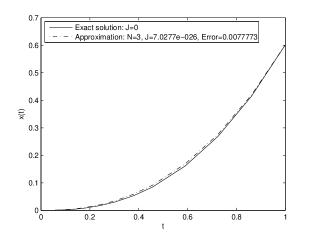
(c) $x(t),N=3$

(d) $u(t),N=3$

Figure 9.2: Exact solution (solid lines) for the problem in Example 69 with $\alpha=1/2$ versus numerical solutions (dashed lines) obtained by approximating the fractional order optimal control problem using (5.10) up to order $N$ and then solving the classical necessary optimality conditions with MATLAB^® bvp4c built-in function.

9.4.2 Free final time

The two numerical methods discussed in Section 9.4.1 are now employed to solve a fractional order optimal control problem with free final time $T$.

Example 70.

Find an optimal triplet $(x(\cdot),u(\cdot),T)$ that minimizes

$$J[x,u,T]=\int_{0}^{T}(tu-(\alpha+2)x)^{2}\,dt$$

subject to the control system

$$\dot{x}(t)+{{}^{C}_{0}D^{\alpha}_{t}}x(t)=u(t)+t^{2}$$

and boundary conditions

$$x(0)=0,\quad x(T)=1.$$

An exact solution to this problem is not known and we apply the two numerical procedures already used with respect to the fixed final time problem in Example 69.

We begin by using the fractional necessary optimality conditions that, after approximating the fractional terms, results in

$$\begin{cases}\displaystyle\dot{x}(t)=\left[\left(\frac{\alpha+2}{t}-At^{-\alpha}\right)x(t)+\sum_{p=2}^{N}C_{p}t^{1-p-\alpha}V_{p}(t)-\frac{\lambda(t)}{2t^{2}}+t^{2}\right]\frac{1}{1+Bt^{1-\alpha}}\\[5.0pt] \dot{V}_{p}(t)=(1-p)t^{p-2}x(t),\quad p=2,\ldots,N\\[5.0pt] \displaystyle\dot{\lambda}(t)=\left[\left(A(1-t)^{-\alpha}-\frac{\alpha+2}{t}\right)\lambda(t)-\sum_{p=2}^{N}C_{p}(1-t)^{1-p-\alpha}W_{p}(t)\right]\frac{1}{1+B(1-t)^{1-\alpha}}\\ \dot{W}_{p}(t)=-(1-p)(1-t)^{p-2}\lambda(t),\quad p=2,\ldots,N,\end{cases}$$

subject to the boundary conditions

$$\begin{cases}x(0)=0,\quad x(T)=1,\\ V_{p}(0)=0,\quad p=2,\ldots,N,\\ W_{p}(T)=0,\quad p=2,\ldots,N.\end{cases}$$

The only difference here with respect to Example 69 is that there is an extra unknown, the terminal time $T$. The boundary condition for this new unknown is chosen appropriately from the transversality conditions discussed in Corollary 61, i.e.,

$$[H(t,x,u,\lambda)-\lambda(t){{}^{C}_{a}D_{t}^{\alpha}}x(t)+\dot{x}(t){{}_{t}I_{T}^{1-\alpha}}\lambda(t)]_{t=T}=0,$$

where $H$ is given as in (9.11). Since we require $\lambda$ to be continuous, ${{}_{t}I_{T}^{1-\alpha}}\lambda(t)|_{t=T}=0$ (cf. [83, pag. 46]) and so $\lambda(T)=0$. One possible way to proceed consists in translating the problem into the interval $[0,1]$ by the change of variable $t=Ts$ [24]. In this setting, either we add $T$ to the problem as a new state variable with dynamics $\dot{T}(s)=0$, or we treat it as a parameter. We use the latter, to get the following parametric boundary value problem:

$$\begin{cases}\displaystyle\dot{x}(s)=\frac{\left[\left(\frac{\alpha+2}{Ts}-A(Ts)^{-\alpha}\right)x(s)+\sum_{p=2}^{N}C_{p}(Ts)^{1-p-\alpha}V_{p}(s)-\frac{\lambda(s)}{2(Ts)^{2}}+(Ts)^{2}\right]T}{1+B(Ts)^{1-\alpha}},\\[5.0pt] \dot{V}_{p}(s)=T(1-p)(Ts)^{p-2}x(s),\quad p=2,\ldots,N,\\[5.0pt] \displaystyle\dot{\lambda}(s)=\frac{\left[\left(A(1-Ts)^{-\alpha}-\frac{\alpha+2}{Ts}\right)\lambda(s)-\sum_{p=2}^{N}C_{p}(1-Ts)^{1-p-\alpha}W_{p}(s)\right]T}{1+B(1-Ts)^{1-\alpha}},\\ \dot{W}_{p}(s)=-T(1-p)(1-Ts)^{p-2}\lambda(s),\quad p=2,\ldots,N,\end{cases}$$

subject to the boundary conditions

$$\begin{cases}x(0)=0\\ V_{p}(0)=0,\quad p=2,\ldots,N\\ W_{p}(1)=0,\quad p=2,\ldots,N\end{cases},\qquad\begin{cases}x(1)=1\\ \lambda(1)=0.\end{cases}$$

This parametric boundary value problem is solved for $N=2$ and $\alpha=0.5$ with MATLAB^® bvp4c function. The result is shown in Figure 9.3 (dashed lines).

(a) $x(t),N=2$

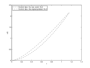
(b) $u(t),N=2$

Figure 9.3: Numerical solutions to the free final time problem of Example 70 with $\alpha=1/2$, using fractional necessary optimality conditions (dashed lines) and approximation of the problem to an integer-order optimal control problem (dash-dotted lines).

We also solve Example 70 with $\alpha=1/2$ by directly transforming it into an integer-order optimal control problem with free final time. As is well known in the classical theory of optimal control, the Hamiltonian must vanish at the terminal point when the final time is free, i.e., one has $H|_{t=T}=0$ with $H$ given by (9.12) [68]. For $N=2$, the necessary optimality conditions give the following two point boundary value problem:

$$\begin{cases}\dot{x}(t)=2\phi_{0}(t)\lambda_{1}(t)+\phi_{1}(t)x(t)+\phi_{2}(t)V_{2}(t)+\phi_{3}(t)\\ \dot{V_{2}}=-x(t)\\ \dot{\lambda_{1}}=-\phi_{1}(t)\lambda_{1}(t)+x(t)\\ \dot{\lambda_{2}}=-\phi_{2}(t)\lambda_{1}(t),\end{cases}$$

where $\phi_{0}(t)$ and $\phi_{1}(t)$ are given by (9.13) and $\phi_{2}(t)$ and $\phi_{3}(t)$ by (9.14) with $p=N=2$. The trajectory $x$ and corresponding $u$ are shown in Figure 9.3 (dash-dotted lines).

Chapter 10 Fractional variational problems depending on indefinite integrals

In this chapter we obtain necessary optimality conditions for variational problems with a Lagrangian depending on a Caputo fractional derivative, a fractional and an indefinite integral. Main results give fractional Euler–Lagrange type equations and natural boundary conditions, which provide a generalization of previous results found in the literature. Isoperimetric problems, problems with holonomic constraints and those depending on higher-order Caputo derivatives, as well as fractional Lagrange problems, are considered. Our main contribution is an extension of the results presented in [4, 58] by considering Lagrangians containing an antiderivative, that in turn depend on the unknown function, a fractional integral, and a Caputo fractional derivative (Section 10.1). Transversality conditions are studied in Section 10.2, where the variational functional $J$ depends also on the terminal time $T$, $J[x,T]$, and where we obtain conditions for a pair $(x,T)$ to be an optimal solution to the problem. In Section 10.3 we consider isoperimetric problems with integral constraints of the same type as the cost functionals considered in Section 10.1. Fractional problems with holonomic constraints are considered in Section 10.4. The situation when the Lagrangian depends on higher order Caputo derivatives, i.e., it depends on ${}^{C}_{a}D_{t}^{\alpha_{k}}x(t)$ for $\alpha_{k}\in(k-1,k)$, $k\in\{1,\ldots,n\}$, is studied in Section 10.5, while Section 10.6 considers fractional Lagrange problems and the Hamiltonian approach. In Section 10.7 we obtain sufficient conditions of optimization under suitable convexity assumptions on the Lagrangian [12].

10.1 The fundamental problem

Let $\alpha\in(0,1)$ and $\beta>0$. The problem that we address is stated in the following way: minimize the cost functional

$$J[x]=\int_{a}^{b}L(t,x(t),{{}^{C}_{a}D_{t}^{\alpha}}x(t),{{}_{a}I_{x}^{\beta}}x(t),z(t))dt,$$ (10.1)

where the variable $z$ is defined by

$$z(t)=\int_{a}^{t}l(\tau,x(\tau),{{}^{C}_{a}D_{\tau}^{\alpha}}x(\tau),{{}_{a}I_{\tau}^{\beta}}x(\tau))d\tau,$$

subject to the boundary conditions

$$x(a)=x_{a}\quad\mbox{and}\quad x(b)=x_{b}.$$ (10.2)

We assume that the functions $(t,x,v,w,z)\to L(t,x,v,w,z)$ and $(t,x,v,w)\to l(t,x,v,w)$ are of class $C^{1}$, and the trajectories $x:[a,b]\to\mathbb{R}$ are absolute continuous functions, $x\in AC([a,b];\mathbb{R})$, such that ${{}^{C}_{a}D_{t}^{\alpha}}x(t)$ and ${{}_{a}I_{t}^{\beta}}x(t)$ exist and are continuous on $[a,b]$. We denote such class of functions by $\mathcal{F}([a,b];\mathbb{R})$. Also, to simplify, by $[\cdot]$ and $\{\cdot\}$ we denote the operators

$$[x](t)=(t,x(t),{{}^{C}_{a}D_{t}^{\alpha}}x(t),{{}_{a}I_{t}^{\beta}}x(t),z(t))\quad\mbox{and}\quad\{x\}(t)=(t,x(t),{{}^{C}_{a}D_{t}^{\alpha}}x(t),{{}_{a}I_{t}^{\beta}}x(t)).$$

Theorem 71.

Let $x\in\mathcal{F}([a,b];\mathbb{R})$ be a minimizer of $J$ as in (10.1), subject to the boundary conditions (10.2). Then, for all $t\in[a,b]$, $x$ is a solution of the fractional equation

$$\frac{\partial L}{\partial x}[x](t)+{{}_{t}D^{\alpha}_{b}}\left(\frac{\partial L}{\partial v}[x](t)\right)+{{}_{t}I_{b}^{\beta}}\left(\frac{\partial L}{\partial w}[x](t)\right)+\int_{t}^{b}\frac{\partial L}{\partial z}[x](\tau)d\tau\cdot\frac{\partial l}{\partial x}\{x\}(t)\\[5.0pt] +{{}_{t}D^{\alpha}_{b}}\left(\int_{t}^{b}\frac{\partial L}{\partial z}[x](\tau)d\tau\cdot\frac{\partial l}{\partial v}\{x\}(t)\right)+{{}_{t}I^{\beta}_{b}}\left(\int_{t}^{b}\frac{\partial L}{\partial z}[x](\tau)d\tau\cdot\frac{\partial l}{\partial w}\{x\}(t)\right)=0.$$ (10.3)

Proof.

Let $h\in\mathcal{F}([a,b];\mathbb{R})$ be such that $h(a)=0=h(b)$, and $\epsilon$ be a real number with $|\epsilon|\ll 1$. If we define $j$ as $j(\epsilon)=J(x+\epsilon h)$, then $j^{\prime}(0)=0$. Differentiating $j$ at $\epsilon=0$, we get

$$\int_{a}^{b}\left[\frac{\partial L}{\partial x}[x](t)h(t)+\frac{\partial L}{\partial v}[x](t){{}^{C}_{a}D^{\alpha}_{t}}h(t)+\frac{\partial L}{\partial w}[x](t){{}_{a}I^{\beta}_{t}}h(t)\right.\\[5.0pt] \left.\;\;+\frac{\partial L}{\partial z}[x](t)\int_{a}^{t}\left(\frac{\partial l}{\partial x}\{x\}(\tau)h(\tau)+\frac{\partial l}{\partial v}\{x\}(\tau){{}^{C}_{a}D^{\alpha}_{\tau}}h(\tau)+\frac{\partial l}{\partial w}\{x\}(\tau){{}_{a}I^{\beta}_{\tau}}h(\tau)\right)d\tau\right]dt=0.$$

The necessary condition (10.3) follows from the next relations and the fundamental lemma of the calculus of variations (cf., e.g., [123, p. 32]):

$$\int_{a}^{b}\frac{\partial L}{\partial v}[x](t){{}^{C}_{a}D^{\alpha}_{t}}h(t)dt=\int_{a}^{b}{{}_{t}D_{b}^{\alpha}}\left(\frac{\partial L}{\partial v}[x](t)\right)h(t)dt+\left[{{}_{t}I_{b}^{1-\alpha}}\left(\frac{\partial L}{\partial v}[x](t)\right)h(t)\right]_{a}^{b},$$

$$\int_{a}^{b}\frac{\partial L}{\partial w}[x](t){{}_{a}I^{\beta}_{t}}h(t)dt=\int_{a}^{b}{{}_{t}I_{b}^{\beta}}\left(\frac{\partial L}{\partial w}[x](t)\right)h(t)dt,$$

$$\int_{a}^{b} \frac{\partial L}{\partial z}[x](t)\left(\int_{a}^{t}\frac{\partial l}{\partial x}\{x\}(\tau)h(\tau)d\tau\right)dt$$

$$=\int_{a}^{b}\left(-\frac{d}{dt}\int_{t}^{b}\frac{\partial L}{\partial z}[x](\tau)d\tau\right)\left(\int_{a}^{t}\frac{\partial l}{\partial x}\{x\}(\tau)h(\tau)d\tau\right)dt$$

$$=\int_{a}^{b}\left(\int_{t}^{b}\frac{\partial L}{\partial z}[x](\tau)d\tau\right)\frac{\partial l}{\partial x}\{x\}(t)h(t)\,dt-\left[\int_{t}^{b}\frac{\partial L}{\partial z}[x](\tau)d\tau\int_{a}^{t}\frac{\partial l}{\partial x}\{x\}(\tau)h(\tau)d\tau\right]_{a}^{b}$$

$$=\int_{a}^{b}\left(\int_{t}^{b}\frac{\partial L}{\partial z}[x](\tau)d\tau\right)\frac{\partial l}{\partial x}\{x\}(t)h(t)\,dt,$$

$$\int_{a}^{b} \frac{\partial L}{\partial z}[x](t)\left(\int_{a}^{t}\frac{\partial l}{\partial v}\{x\}(\tau){{}^{C}_{a}D^{\alpha}_{\tau}}h(\tau)d\tau\right)dt$$

$$\hskip 56.9055pt=\int_{a}^{b}\left(-\frac{d}{dt}\int_{t}^{b}\frac{\partial L}{\partial z}[x](\tau)d\tau\right)\left(\int_{a}^{t}\frac{\partial l}{\partial v}\{x\}(\tau){{}^{C}_{a}D^{\alpha}_{\tau}}h(\tau)d\tau\right)dt$$

$$\hskip 56.9055pt=\left[-\left(\int_{t}^{b}\frac{\partial L}{\partial z}[x](\tau)d\tau\right)\left(\int_{a}^{t}\frac{\partial l}{\partial v}\{x\}(\tau){{}^{C}_{a}D^{\alpha}_{\tau}}h(\tau)d\tau\right)\right]_{a}^{b}$$

$$\hskip 85.35826pt+\int_{a}^{b}\left(\int_{t}^{b}\frac{\partial L}{\partial z}[x](\tau)d\tau\right)\frac{\partial l}{\partial v}\{x\}(t){{}^{C}_{a}D^{\alpha}_{t}}h(t)\,dt$$

$$\hskip 56.9055pt=\int_{a}^{b}{{}_{t}D^{\alpha}_{b}}\left(\int_{t}^{b}\frac{\partial L}{\partial z}[x](\tau)d\tau\frac{\partial l}{\partial v}\{x\}(t)\right)h(t)\,dt$$

$$\hskip 85.35826pt+\left[{{}_{t}I^{1-\alpha}_{b}}\left(\int_{t}^{b}\frac{\partial L}{\partial z}[x](\tau)d\tau\frac{\partial l}{\partial v}\{x\}(t)\right)h(t)\right]_{a}^{b},$$

and

$$\int_{a}^{b}\frac{\partial L}{\partial z}[x](t)\left(\int_{a}^{t}\frac{\partial l}{\partial w}\{x\}(t){{}_{a}I^{\beta}_{\tau}}h(\tau)d\tau\right)dt=\int_{a}^{b}{{}_{t}I^{\beta}_{b}}\left(\int_{t}^{b}\frac{\partial L}{\partial z}[x](\tau)d\tau\frac{\partial l}{\partial w}\{x\}(t)\right)h(t)\,dt.$$

∎

The fractional Euler–Lagrange equation (10.3) involves not only fractional integrals and fractional derivatives, but also indefinite integrals. Theorem 71 gives a necessary condition to determine the possible choices for extremizers.

Example 72.

Consider the functional

$$J[x]=\int_{0}^{1}\left[({{}^{C}_{0}D_{t}^{\alpha}}x(t)-\Gamma(\alpha+2)t)^{2}+z(t)\right]dt,$$ (10.4)

where $\alpha\in(0,1)$ and

$$z(t)=\int_{0}^{t}(x(\tau)-\tau^{\alpha+1})^{2}\,d\tau,$$

defined on the set

$$\left\{x\in\mathcal{F}([0,1];\mathbb{R}):\,x(0)=0\,\mbox{ and }\,x(1)=1\right\}.$$

Let

$$x_{\alpha}(t)=t^{\alpha+1},\quad t\in[0,1].$$ (10.5)

Then,

$${{}^{C}_{0}D_{t}^{\alpha}}x_{\alpha}(t)=\Gamma(\alpha+2)t.$$

Since $J(x)\geq 0$ for all admissible functions $x$, and $J(x_{\alpha})=0$, we have that $x_{\alpha}$ is a minimizer of $J$. The Euler–Lagrange equation applied to (10.4) gives

$${{}_{t}D_{1}^{\alpha}}({{}^{C}_{0}D_{t}^{\alpha}}x(t)-\Gamma(\alpha+2)t)+\int_{t}^{1}1dt\,(x(t)-t^{\alpha+1})=0.$$ (10.6)

Obviously, $x_{\alpha}$ is a solution of the fractional differential equation (10.6).

The extremizer (10.5) of Example 72 is smooth on the closed interval $[0,1]$. This is not always the case. As next example shows, minimizers of (10.1)–(10.2) are not necessarily $C^{1}$ functions.

Example 73.

Consider the following fractional variational problem: to minimize the functional

$$J[x]=\int_{0}^{1}\left[\left({{}^{C}_{0}D_{t}^{\alpha}}x(t)-1\right)^{2}+z(t)\right]dt,$$ (10.7)

on

$$\left\{x\in\mathcal{F}([0,1];\mathbb{R})\,:\,x(0)=0\quad\mbox{and}\quad x(1)=\frac{1}{\Gamma(\alpha+1)}\right\},$$

where $z$ is given by

$$z(t)=\int_{0}^{t}\left(x(\tau)-\frac{\tau^{\alpha}}{\Gamma(\alpha+1)}\right)^{2}d\tau.$$

Since ${{}^{C}_{0}D_{t}^{\alpha}}t^{\alpha}=\Gamma(\alpha+1)$, we deduce easily that function

$$\overline{x}(t)=\frac{t^{\alpha}}{\Gamma(\alpha+1)}$$ (10.8)

is the global minimizer to the problem. Indeed, $J(x)\geq 0$ for all $x$, and $J(\overline{x})=0$. Let us see that $\overline{x}$ is an extremal for $J$. The fractional Euler–Lagrange equation (10.3) becomes

$$2\,{{}_{t}D_{1}^{\alpha}}({{}^{C}_{0}D_{t}^{\alpha}}x(t)-1)+\int_{t}^{1}1\,d\tau\cdot 2\left(x(t)-\frac{t^{\alpha}}{\Gamma(\alpha+1)}\right)=0.$$ (10.9)

Obviously, $\overline{x}$ is a solution of equation (10.9).

Remark 74.

The minimizer (10.8) of Example 73 is not differentiable at 0, as $0<\alpha<1$. However, $\overline{x}(0)=0$ and ${{}^{C}_{0}D_{t}^{\alpha}}\overline{x}(t)={{}_{0}D_{t}^{\alpha}}\overline{x}(t)=\Gamma(\alpha+1)$ for any $t\in[0,1]$.

Corollary 75 (cf. equation (9) of [4]).

If $x$ is a minimizer of

$$J[x]=\int_{a}^{b}L(t,x(t),{{}^{C}_{a}D_{t}^{\alpha}}x(t))dt,$$ (10.10)

subject to the boundary conditions (10.2), then $x$ is a solution of the fractional equation

$$\frac{\partial L}{\partial x}[x](t)+{{}_{t}D^{\alpha}_{b}}\left(\frac{\partial L}{\partial v}[x](t)\right)=0.$$

Proof.

Follows from Theorem 71 with an $L$ that does not depend on ${{}_{a}I_{t}^{\beta}}x$ and $z$. ∎

We now derive the Euler–Lagrange equations for functionals containing several dependent variables, i.e., for functionals of type

$$J[x_{1},\ldots,x_{n}]=\int_{a}^{b}L(t,x_{1},\ldots,x_{n},{{}^{C}_{a}D_{t}^{\alpha}}x_{1},\ldots,{{}^{C}_{a}D_{t}^{\alpha}}x_{n},{{}_{a}I_{t}^{\beta}}x_{1},\ldots,{{}_{a}I_{t}^{\beta}}x_{n},z(t))dt,$$ (10.11)

where $n\in\mathbb{N}$ and $z$ is defined by

$$z(t)=\int_{a}^{t}l(\tau,x_{1}(\tau),\ldots,x_{n}(\tau),{{}^{C}_{a}D_{\tau}^{\alpha}}x_{1}(\tau),\ldots,{{}^{C}_{a}D_{\tau}^{\alpha}}x_{n}(\tau),{{}_{a}I_{\tau}^{\beta}}x_{1}(\tau),\ldots,{{}_{a}I_{t}^{\beta}}x_{n}(\tau))d\tau,$$

subject to the boundary conditions

$$x_{k}(a)=x_{a,k}\quad\mbox{and}\quad x_{k}(b)=x_{b,k},\quad k\in\{1,\ldots,n\}.$$ (10.12)

To simplify, we consider $x$ as the vector $x=(x_{1},\ldots,x_{n})$. Consider a family of variations $x+\epsilon h$, where $|\epsilon|\ll 1$ and $h=(h_{1},\ldots,h_{n})$. The boundary conditions (10.12) imply that $h_{k}(a)=0=h_{k}(b)$, for $k\in\{1,\ldots,n\}$. The following theorem can be easily proved.

Theorem 76.

Let $x$ be a minimizer of $J$ as in (10.11), subject to the boundary conditions (10.12). Then, for all $k\in\{1,\ldots,n\}$ and for all $t\in[a,b]$, $x$ is a solution of the fractional Euler–Lagrange equation

$$\frac{\partial L}{\partial x_{k}}[x](t)+{{}_{t}D^{\alpha}_{b}}\left(\frac{\partial L}{\partial v_{k}}[x](t)\right)+{{}_{t}I^{\beta}_{b}}\left(\frac{\partial L}{\partial w_{k}}[x](t)\right)+\int_{t}^{b}\frac{\partial L}{\partial z}[x](\tau)d\tau\cdot\frac{\partial l}{\partial x_{k}}\{x\}(t)\\ +{{}_{t}D^{\alpha}_{b}}\left(\int_{t}^{b}\frac{\partial L}{\partial z}[x](\tau)d\tau\cdot\frac{\partial l}{\partial v_{k}}\{x\}(t)\right)+{{}_{t}I^{\beta}_{b}}\left(\int_{t}^{b}\frac{\partial L}{\partial z}[x](\tau)d\tau\cdot\frac{\partial l}{\partial w_{k}}\{x\}(t)\right)=0.$$

10.2 Natural boundary conditions

In this section we consider a more general question. Not only the unknown function $x$ is a variable in the problem, but also the terminal time $T$ is an unknown. For $T\in[a,b]$, consider the functional

$$J[x,T]=\int_{a}^{T}L[x](t)dt,$$ (10.13)

where

$$[x](t)=(t,x(t),{{}^{C}_{a}D_{t}^{\alpha}}x(t),{{}_{a}I_{t}^{\beta}}x(t),z(t)).$$

The problem consists in finding a pair $(x,T)\in\mathcal{F}([a,b];\mathbb{R})\times[a,b]$ for which the functional $J$ attains a minimum value. First we recall a property that will be used later in the proof of Theorem 78.

Remark 77.

If $\phi$ is a continuous function, then (cf. [83, p. 46])

$$\lim_{t\to T}{{}_{t}I_{T}^{1-\alpha}}\phi(t)=0$$

for any $\alpha\in(0,1)$.

Theorem 78.

Let $(x,T)$ be a minimizer of $J$ as in (10.13). Then, for all $t\in[a,T]$, $(x,T)$ is a solution of the fractional equation

$$\frac{\partial L}{\partial x}[x](t)+{{}_{t}D^{\alpha}_{T}}\left(\frac{\partial L}{\partial v}[x](t)\right)+{{}_{t}I_{T}^{\beta}}\left(\frac{\partial L}{\partial w}[x](t)\right)+\int_{t}^{T}\frac{\partial L}{\partial z}[x](t)dt\cdot\frac{\partial l}{\partial x}\{x\}(t)\\ +{{}_{t}D^{\alpha}_{T}}\left(\int_{t}^{T}\frac{\partial L}{\partial z}[x](\tau)d\tau\cdot\frac{\partial l}{\partial v}\{x\}(t)\right)+{{}_{t}I^{\beta}_{T}}\left(\int_{t}^{T}\frac{\partial L}{\partial z}[x](\tau)d\tau\cdot\frac{\partial l}{\partial w}\{x\}(t)\right)=0$$

and satisfies the transversality conditions

$$\left[{{}_{t}I_{T}^{1-\alpha}}\left(\frac{\partial L}{\partial v}[x](t)+\int_{t}^{T}\frac{\partial L}{\partial z}[x](\tau)\,d\tau\cdot\frac{\partial l}{\partial v}\{x\}(t)\right)\right]_{t=a}=0$$

and

$$L[x](T)=0.$$

Proof.

Let $h\in\mathcal{F}([a,b];\mathbb{R})$ be a variation, and let $\triangle T$ be a real number. Define the function

$$j(\epsilon)=J[x+\epsilon h,T+\epsilon\triangle T]$$

with $|\epsilon|\ll 1$. Differentiating $j$ at $\epsilon=0$, and using the same procedure as in Theorem 71, we deduce that

$$0= \triangle T\cdot L[x](T)+\int_{a}^{T}\left[\frac{\partial L}{\partial x}[x](t)+{{}_{t}D^{\alpha}_{T}}\left(\frac{\partial L}{\partial v}[x](t)\right)+{{}_{t}I_{T}^{\beta}}\left(\frac{\partial L}{\partial w}[x](t)\right)\right.$$

$$\left.\hskip 99.58464pt+\int_{t}^{T}\frac{\partial L}{\partial z}[x](\tau)d\tau\cdot\frac{\partial l}{\partial x}\{x\}(t)+{{}_{t}D^{\alpha}_{T}}\left(\int_{t}^{T}\frac{\partial L}{\partial z}[x](\tau)d\tau\cdot\frac{\partial l}{\partial v}\{x\}(t)\right)\right.$$

$$\left.\hskip 99.58464pt+{{}_{t}I^{\beta}_{T}}\left(\int_{t}^{T}\frac{\partial L}{\partial z}[x](\tau)d\tau\cdot\frac{\partial l}{\partial w}\{x\}(t)\right)\right]h(t)dt$$

$$+\left[{{}_{t}I_{T}^{1-\alpha}}\left(\frac{\partial L}{\partial v}[x](t)\right)h(t)\right]_{a}^{T}+\left[{{}_{t}I^{1-\alpha}_{T}}\left(\int_{t}^{T}\frac{\partial L}{\partial z}[x](\tau)d\tau\cdot\frac{\partial l}{\partial v}\{x\}(t)\right)h(t)\right]_{a}^{T}.$$

The theorem follows from the arbitrariness of $h$ and $\triangle T$. ∎

Remark 79.

If $T$ is fixed, say $T=b$, then $\triangle T=0$ and the transversality conditions reduce to

$$\left[{{}_{t}I_{b}^{1-\alpha}}\left(\frac{\partial L}{\partial v}[x](t)+\int_{t}^{b}\frac{\partial L}{\partial z}[x](\tau)\,d\tau\cdot\frac{\partial l}{\partial v}\{x\}(t)\right)\right]_{a}=0.$$ (10.14)

Example 80.

Consider the problem of minimizing the functional $J$ as in (10.7), but without given boundary conditions. Besides equation (10.9), extremals must also satisfy

$$\left[{{}_{t}I_{1}^{1-\alpha}}\left({{}^{C}_{0}D_{t}^{\alpha}}x(t)-1\right)\right]_{0}=0.$$ (10.15)

Again, $\overline{x}$ given by (10.8) is a solution of (10.9) and (10.15).

As a particular case, the following result of [4] is deduced.

Corollary 81 (cf. equations (9) and (12) of [4]).

If $x$ is a minimizer of $J$ as in (10.10), then $x$ is a solution of

$$\frac{\partial L}{\partial x}[x](t)+{{}_{t}D^{\alpha}_{b}}\left(\frac{\partial L}{\partial v}[x](t)\right)=0,$$

and satisfies the transversality condition

$$\left[{{}_{t}I_{b}^{1-\alpha}}\left(\frac{\partial L}{\partial v}[x](t)\right)\right]_{a}=0.$$

Proof.

The Lagrangian $L$ in (10.10) does not depend on ${{}_{a}I_{t}^{\beta}}x$ and $z$, and the result follows from Theorem 78. ∎

Remark 82.

Observe that the condition

$$\left[{{}_{t}I_{b}^{1-\alpha}}\left(\frac{\partial L}{\partial v}[x](t)\right)\right]_{b}=0$$

is implicitly satisfied in Corollary 81 (cf. Remark 77).

10.3 Fractional isoperimetric problems

An isoperimetric problem deals with the question of optimizing a given functional under the presence of an integral constraint. This is a very old question, with its origins in the ancient Greece. They where interested in determining the shape of a closed curve with a fixed length and maximum area. This problem is known as Dido’s problem, and is an example of an isoperimetric problem of the calculus of variations [123]. For recent advancements on the subject we refer the reader to [14, 15, 48, 76] and references therein. In our case, within the fractional context, we state the isoperimetric problem in the following way. Determine the minimizers of a given functional

$$J[x]=\int_{a}^{b}L(t,x(t),{{}^{C}_{a}D_{t}^{\alpha}}x(t),{{}_{a}I_{t}^{\beta}}x(t),z(t))dt,$$ (10.16)

subject to the boundary conditions

$$x(a)=x_{a}\quad\mbox{and}\quad x(b)=x_{b},$$ (10.17)

and the fractional integral constraint

$$\int_{a}^{b}G(t,x(t),{{}^{C}_{a}D_{t}^{\alpha}}x(t),{{}_{a}I_{t}^{\beta}}x(t),z(t))dt=\gamma,\quad\gamma\in\mathbb{R},$$ (10.18)

where $z$ is defined by

$$z(t)=\int_{a}^{t}l(\tau,x(\tau),{{}^{C}_{a}D_{\tau}^{\alpha}}x(\tau),{{}_{a}I_{\tau}^{\beta}}x(\tau))d\tau.$$

As usual, we assume that all the functions $(t,x,v,w,z)\to L(t,x,v,w,z)$, $(t,x,v,w)\to l(t,x,v,w)$, and $(t,x,v,w,z)\to G(t,x,v,w,z)$ are of class $C^{1}$.

Theorem 83.

Let $x$ be a minimizer of $J$ as in (10.16), under the boundary conditions (10.17) and isoperimetric constraint (10.18). Suppose that $x$ is not an extremal for $I$ in (10.18). Then there exists a constant $\lambda$ such that $x$ is a solution of the fractional equation

$$\frac{\partial F}{\partial x}[x](t)+{{}_{t}D^{\alpha}_{b}}\left(\frac{\partial F}{\partial v}[x](t)\right)+{{}_{t}I^{\beta}_{b}}\left(\frac{\partial F}{\partial w}[x](t)\right)+\int_{t}^{b}\frac{\partial F}{\partial z}[x](\tau)d\tau\cdot\frac{\partial l}{\partial x}\{x\}(t)\\ +{{}_{t}D^{\alpha}_{b}}\left(\int_{t}^{b}\frac{\partial F}{\partial z}[x](\tau)d\tau\cdot\frac{\partial l}{\partial v}\{x\}(t)\right)+{{}_{t}I^{\beta}_{b}}\left(\int_{t}^{b}\frac{\partial F}{\partial z}[x](\tau)d\tau\cdot\frac{\partial l}{\partial w}\{x\}(t)\right)=0,$$

where $F=L-\lambda G$, for all $t\in[a,b]$.

Proof.

Let $\epsilon_{1},\epsilon_{2}\in\mathbb{R}$ be two real numbers such that $|\epsilon_{1}|\ll 1$ and $|\epsilon_{2}|\ll 1$, with $\epsilon_{1}$ free and $\epsilon_{2}$ to be determined later, and let $h_{1}$ and $h_{2}$ be two functions satisfying

$$h_{1}(a)=h_{1}(b)=h_{2}(a)=h_{2}(b)=0.$$

Define functions $j$ and $i$ by

$$j(\epsilon_{1},\epsilon_{2})=J[x+\epsilon_{1}h_{1}+\epsilon_{2}h_{2}]$$

and

$$i(\epsilon_{1},\epsilon_{2})=I(x+\epsilon_{1}h_{1}+\epsilon_{2}h_{2})-\gamma.$$

Doing analogous calculations as in the proof of Theorem 71, one has

$$\left.\frac{\partial i}{\partial\epsilon_{2}}\right|_{(0,0)}= \int_{a}^{b}\left[\frac{\partial G}{\partial x}[x](t)+\int_{t}^{b}\frac{\partial G}{\partial z}[x](\tau)d\tau\cdot\frac{\partial l}{\partial x}\{x\}(t)\right.$$

$$\hskip 28.45274pt\left.+{{}_{t}D^{\alpha}_{b}}\left(\frac{\partial G}{\partial v}[x](t)\right)+{{}_{t}D^{\alpha}_{b}}\left(\int_{t}^{b}\frac{\partial G}{\partial z}[x](\tau)d\tau\cdot\frac{\partial l}{\partial v}\{x\}(t)\right)\right.$$

$$\hskip 28.45274pt\left.+{{}_{t}I^{\alpha}_{b}}\left(\frac{\partial G}{\partial w}[x](t)\right)+{{}_{t}I^{\beta}_{b}}\left(\int_{t}^{b}\frac{\partial G}{\partial z}[x](\tau)d\tau\cdot\frac{\partial l}{\partial w}\{x\}(t)\right)\right]h_{2}(t)\,dt.$$

By hypothesis, $x$ is not an extremal for $I$ and therefore there must exist a function $h_{2}$ for which

$$\left.\frac{\partial i}{\partial\epsilon_{2}}\right|_{(0,0)}\not=0.$$

Since $i(0,0)=0$, by the implicit function theorem there exists a function $\epsilon_{2}(\cdot)$, defined in some neighborhood of zero, such that

$$i(\epsilon_{1},\epsilon_{2}(\epsilon_{1}))=0.$$ (10.19)

On the other hand, $j$ attains a minimum value at $(0,0)$ when subject to the constraint (10.19). Because $\nabla i(0,0)\neq(0,0)$, by the Lagrange multiplier rule [123, p. 77] there exists a constant $\lambda$ such that

$$\nabla(j(0,0)-\lambda i(0,0))=(0,0).$$

So

$$\left.\frac{\partial j}{\partial\epsilon_{1}}\right|_{(0,0)}-\lambda\left.\frac{\partial i}{\partial\epsilon_{1}}\right|_{(0,0)}=0.$$

Differentiating $j$ and $i$ at zero, and doing the same calculations as before, we get the desired result. ∎

Using the abnormal Lagrange multiplier rule [123, p. 82], the previous result can be generalized to include the case when the minimizer is an extremal of $I$.

Theorem 84.

Let $x$ be a minimizer of $J$ as in (10.16), subject to the constraints (10.17) and (10.18). Then there exist two constants $\lambda_{0}$ and $\lambda$, not both zero, such that $x$ is a solution of equation

$$\frac{\partial K}{\partial x}[x](t)+{{}_{t}D^{\alpha}_{b}}\left(\frac{\partial K}{\partial v}[x](t)\right)+{{}_{t}I^{\beta}_{b}}\left(\frac{\partial K}{\partial w}[x](t)\right)+\int_{t}^{b}\frac{\partial K}{\partial z}[x](t)dt\cdot\frac{\partial l}{\partial x}\{x\}(t)\\ +{{}_{t}D^{\alpha}_{b}}\left(\int_{t}^{b}\frac{\partial K}{\partial z}[x](\tau)d\tau\cdot\frac{\partial l}{\partial v}\{x\}(t)\right)+{{}_{t}I^{\beta}_{b}}\left(\int_{t}^{b}\frac{\partial K}{\partial z}[x](\tau)d\tau\cdot\frac{\partial l}{\partial w}\{x\}(t)\right)=0$$

for all $t\in[a,b]$, where $K=\lambda_{0}L-\lambda G$.

Corollary 85 (cf. Theorem 3.4 of [17]).

Let $x$ be a minimizer of

$$J[x]=\int_{a}^{b}L(t,x(t),{{}^{C}_{a}D_{t}^{\alpha}}x(t))dt,$$

subject to the boundary conditions

$$x(a)=x_{a}\quad\mbox{and}\quad x(b)=x_{b},$$

and the isoperimetric constraint

$$\int_{a}^{b}G(t,x(t),{{}^{C}_{a}D_{t}^{\alpha}}x(t))dt=\gamma,\quad\gamma\in\mathbb{R}.$$

Then, there exist two constants $\lambda_{0}$ and $\lambda$, not both zero, such that $x$ is a solution of equation

$$\frac{\partial K}{\partial x}\left(t,x(t),{{}^{C}_{a}D_{t}^{\alpha}}x(t)\right)+{{}_{t}D^{\alpha}_{b}}\left(\frac{\partial K}{\partial v}\left(t,x(t),{{}^{C}_{a}D_{t}^{\alpha}}x(t)\right)\right)=0$$

for all $t\in[a,b]$, where $K=\lambda_{0}L-\lambda G$. Moreover, if $x$ is not an extremal for $I$, then we may take $\lambda_{0}=1$.

10.4 Holonomic constraints

In this section we consider the following problem. Minimize the functional

$$J[x_{1},x_{2}]=\int_{a}^{b}L(t,x_{1}(t),x_{2}(t),{{}^{C}_{a}D_{t}^{\alpha}}x_{1}(t),{{}^{C}_{a}D_{t}^{\alpha}}x_{2}(t),{{}_{a}I_{t}^{\beta}}x_{1}(t),{{}_{a}I_{t}^{\beta}}x_{2}(t),z(t))dt,$$ (10.20)

where $z$ is defined by

$$z(t)=\int_{a}^{t}l(t,x_{1}(\tau),x_{2}(\tau),{{}^{C}_{a}D_{\tau}^{\alpha}}x_{1}(\tau),{{}^{C}_{a}D_{\tau}^{\alpha}}x_{2}(\tau),{{}_{a}I_{\tau}^{\beta}}x_{1}(\tau),{{}_{a}I_{\tau}^{\beta}}x_{2}(\tau))d\tau,$$

when restricted to the boundary conditions

$$(x_{1}(a),x_{2}(a))=(x_{1}^{a},x_{2}^{a})\mbox{ and }(x_{1}(b),x_{2}(b))=(x_{1}^{b},x_{2}^{b}),\quad x_{1}^{a},x_{2}^{a},x_{1}^{b},x_{2}^{b}\in\mathbb{R},$$ (10.21)

and the holonomic constraint

$$g(t,x_{1}(t),x_{2}(t))=0.$$ (10.22)

As usual, here

$$(t,x_{1},x_{2},v_{1},v_{2},w_{1},w_{2},z)\to L(t,x_{1},x_{2},v_{1},v_{2},w_{1},w_{2},z),$$

$$(t,x_{1},x_{2},v_{1},v_{2},w_{1},w_{2})\to l(t,x_{1},x_{2},v_{1},v_{2},w_{1},w_{2})$$

and

$$(t,x_{1},x_{2})\to g(t,x_{1},x_{2})$$

are all smooth. In what follows we make use of the operator $[\cdot,\cdot]$ given by

$$[x_{1},x_{2}](t)=(t,x_{1}(t),x_{2}(t),{{}^{C}_{a}D_{t}^{\alpha}}x_{1}(t),{{}^{C}_{a}D_{t}^{\alpha}}x_{2}(t),{{}_{a}I_{t}^{\beta}}x_{1}(t),{{}_{a}I_{t}^{\beta}}x_{2}(t),z(t))\,,$$

we denote $(t,x_{1}(t),x_{2}(t))$ by $(t,\mathbf{x}(t))$, and the Euler–Lagrange equation obtained in (10.3) with respect to $x_{i}$ by $(ELE_{i})$, $i=1,2$.

Remark 86.

For simplicity, we are considering functionals depending only on two functions $x_{1}$ and $x_{2}$. Theorem 87 is, however, easily generalized for $n$ variables $x_{1},\ldots,x_{n}$.

Theorem 87.

Let the pair $(x_{1},x_{2})$ be a minimizer of $J$ as in (10.20), subject to the constraints (10.21)–(10.22). If $\frac{\partial g}{\partial x_{2}}\not=0$, then there exists a continuous function $\lambda:[a,b]\to\mathbb{R}$ such that $(x_{1},x_{2})$ is a solution of

$$\frac{\partial F}{\partial x_{i}}[x_{1},x_{2}](t)+\int_{t}^{b}\frac{\partial F}{\partial z}[x_{1},x_{2}](\tau)d\tau\cdot\frac{\partial l}{\partial x_{i}}\{x_{1},x_{2}\}(t)\\ +{{}_{t}D^{\alpha}_{b}}\left(\frac{\partial F}{\partial v_{i}}[x_{1},x_{2}](t)\right)+{{}_{t}D^{\alpha}_{b}}\left(\int_{t}^{b}\frac{\partial F}{\partial z}[x_{1},x_{2}](\tau)d\tau\cdot\frac{\partial l}{\partial v_{i}}\{x_{1},x_{2}\}(t)\right)\\ ~{}~{}+{{}_{t}I_{b}^{\beta}}\left(\frac{\partial F}{\partial w_{i}}[x_{1},x_{2}](t)\right)+{{}_{t}I^{\beta}_{b}}\left(\int_{t}^{b}\frac{\partial F}{\partial z}[x_{1},x_{2}](\tau)d\tau\cdot\frac{\partial l}{\partial w_{i}}\{x_{1},x_{2}\}(t)\right)=0$$ (10.23)

for all $t\in[a,b]$ and $i=1,2$, where $F[x_{1},x_{2}](t)=L[x_{1},x_{2}](t)-\lambda(t)g(t,\mathbf{x}(t))$.

Proof.

Consider a variation of the optimal solution of type

$$(\overline{x}_{1},\overline{x}_{2})=(x_{1}+\epsilon h_{1},x_{2}+\epsilon h_{2}),$$

where $h_{1},h_{2}$ are two functions defined on $[a,b]$ satisfying

$$h_{1}(a)=h_{1}(b)=h_{2}(a)=h_{2}(b)=0,$$

and $\epsilon$ is a sufficiently small real parameter. Since $\frac{\partial g}{\partial x_{2}}(t,\overline{x}_{1}(t),\overline{x}_{2}(t))\not=0$ for all $t\in[a,b]$, we can solve equation $g(t,\overline{x}_{1}(t),\overline{x}_{2}(t))=0$ with respect to $h_{2}$, $h_{2}=h_{2}(\epsilon,h_{1})$. Differentiating $J(\overline{x}_{1},\overline{x}_{2})$ at $\epsilon=0$, and proceeding similarly as done in the proof of Theorem 71, we deduce that

$$\int_{a}^{b}(ELE_{1})h_{1}(t)+(ELE_{2})h_{2}(t)\,dt=0.$$ (10.24)

Besides, since $g(t,\overline{x}_{1}(t),\overline{x}_{2}(t))=0$, differentiating at $\epsilon=0$ we get

$$h_{2}(t)=-\frac{\frac{\partial g}{\partial x_{1}}(t,\mathbf{x}(t))}{\frac{\partial g}{\partial x_{2}}(t,\mathbf{x}(t))}h_{1}(t).$$ (10.25)

Define the function $\lambda$ on $[a,b]$ as

$$\lambda(t)=\frac{(ELE_{2})}{\frac{\partial g}{\partial x_{2}}(t,\mathbf{x}(t))}.$$ (10.26)

Combining (10.25) and (10.26), equation (10.24) can be written as

$$\int_{a}^{b}\left[(ELE_{1})-\lambda(t)\frac{\partial g}{\partial x_{1}}(t,\mathbf{x}(t))\right]h_{1}(t)\,dt=0.$$

By the arbitrariness of $h_{1}$, if follows that

$$(ELE_{1})-\lambda(t)\frac{\partial g}{\partial x_{1}}(t,\mathbf{x}(t))=0.$$

Define $F$ as

$$F[x_{1},x_{2}](t)=L[x_{1},x_{2}](t)-\lambda(t)g(t,\mathbf{x}(t)).$$

Then, equations (10.23) follow. ∎

10.5 Higher order Caputo derivatives

In this section we consider fractional variational problems in presence of higher order Caputo derivatives. We will restrict ourselves to the case where the orders are non-integer, since the integer case is already well studied in the literature (for a modern account see [32, 47, 80]).

Let $n\in\mathbb{N}$, $\beta>0$, and $\alpha_{k}\in\mathbb{R}$ be such that $\alpha_{k}\in(k-1,k)$ for $k\in\{1,\ldots,n\}$. Admissible functions $x$ belong to $AC^{n}([a,b];\mathbb{R})$ and are such that ${{}^{C}_{a}D_{t}^{\alpha_{k}}}x$, $k=1,\ldots,n$, and ${{}_{a}I_{t}^{\beta}}x$ exist and are continuous on $[a,b]$. We denote such class of functions by $\mathcal{F}^{n}([a,b];\mathbb{R})$. For $\alpha=(\alpha_{1},\ldots,\alpha_{n})$, define the vector

$${{}_{a}^{C}D_{t}^{\alpha}}x(t)=({{}_{a}^{C}D_{t}^{\alpha_{1}}}x(t),\ldots,{{}_{a}^{C}D_{t}^{\alpha_{n}}}x(t)).$$ (10.27)

The optimization problem is the following: to minimize or maximize the functional

$$J[x]=\int_{a}^{b}L(t,x(t),{{}^{C}_{a}D_{t}^{\alpha}}x(t),{{}_{a}I_{t}^{\beta}}x(t),z(t))dt,$$ (10.28)

$x\in\mathcal{F}^{n}([a,b];\mathbb{R})$, subject to the boundary conditions

$$x^{(k)}(a)=x_{a,k}\quad\mbox{and}\quad x^{(k)}(b)=x_{b,k},\quad k\in\{0,\ldots,n-1\},$$ (10.29)

where $z:[a,b]\to\mathbb{R}$ is defined by

$$z(t)=\int_{a}^{t}l(\tau,x(\tau),{{}^{C}_{a}D_{\tau}^{\alpha}}x(\tau),{{}_{a}I_{\tau}^{\beta}}x(\tau))d\tau.$$

Theorem 88.

If $x\in\mathcal{F}^{n}([a,b];\mathbb{R})$ is a minimizer of $J$ as in (10.28), subject to the boundary conditions (10.29), then $x$ is a solution of the fractional equation

$$\frac{\partial L}{\partial x}[x](t)+\sum_{k=1}^{n}{{}_{t}D^{\alpha_{k}}_{b}}\left(\frac{\partial L}{\partial v_{k}}[x](t)\right)+{{}_{t}I^{\beta}_{b}}\left(\frac{\partial L}{\partial w}[x](t)\right)+\int_{t}^{b}\frac{\partial L}{\partial z}[x](t)dt\cdot\frac{\partial l}{\partial x}\{x\}(t)\\ +\sum_{k=1}^{n}{{}_{t}D^{\alpha_{k}}_{b}}\left(\int_{t}^{b}\frac{\partial L}{\partial z}[x](\tau)d\tau\cdot\frac{\partial l}{\partial v_{k}}\{x\}(t)\right)+{{}_{t}I^{\beta}_{b}}\left(\int_{t}^{b}\frac{\partial L}{\partial z}[x](\tau)d\tau\cdot\frac{\partial l}{\partial w}\{x\}(t)\right)=0$$

for all $t\in[a,b]$, where $[x](t)=\left(t,x(t),{{}^{C}_{a}D_{t}^{\alpha}}x(t),{{}_{a}I_{t}^{\beta}}x(t),z(t)\right)$ with ${{}^{C}_{a}D_{t}^{\alpha}}x(t)$ as in (10.27).

Proof.

Let $h\in\mathcal{F}^{n}([a,b];\mathbb{R})$ be such that $h^{(k)}(a)=h^{(k)}(b)=0$, for $k\in\{0,\ldots,n-1\}$. Define the new function $j$ as $j(\epsilon)=J(x+\epsilon h)$. Then

$$0=\int_{a}^{b}\left[\frac{\partial L}{\partial x}[x](t)h(t)+\sum_{k=1}^{n}\frac{\partial L}{\partial v_{k}}[x](t){{}^{C}_{a}D^{\alpha_{k}}_{t}}h(t)+\frac{\partial L}{\partial w}[x](t){{}_{a}I^{\beta}_{t}}h(t)\right.\\ \left.+\frac{\partial L}{\partial z}[x](t)\int_{a}^{t}\left(\frac{\partial l}{\partial x}\{x\}(\tau)h(\tau)+\sum_{k=1}^{n}\frac{\partial l}{\partial v_{k}}\{x\}(\tau){{}^{C}_{a}D^{\alpha_{k}}_{\tau}}h(\tau)+\frac{\partial l}{\partial w}\{x\}(\tau){{}_{a}I^{\beta}_{\tau}}h(\tau)\right)d\tau\right]dt.$$ (10.30)

Integrating by parts, we get that

$$\int_{a}^{b}\frac{\partial L}{\partial v_{k}}[x](t){{}^{C}_{a}D^{\alpha_{k}}_{t}}h(t)dt=\int_{a}^{b}{{}_{t}D_{b}^{\alpha_{k}}}\left(\frac{\partial L}{\partial v_{k}}[x](t)\right)h(t)dt\\ +\sum_{m=0}^{k-1}\left[{{}_{t}D_{b}^{\alpha_{k}+m-k}}\left(\frac{\partial L}{\partial v_{k}}[x](t)\right)h^{(k-1-m)}(t)\right]_{a}^{b}=\int_{a}^{b}{{}_{t}D_{b}^{\alpha_{k}}}\left(\frac{\partial L}{\partial v_{k}}[x](t)\right)h(t)dt$$

for all $k\in\{1,\ldots,n\}$. Moreover, one has

$$\int_{a}^{b}\frac{\partial L}{\partial w}[x](t){{}_{a}I^{\beta}_{t}}h(t)dt=\int_{a}^{b}{{}_{t}I_{b}^{\beta}}\left(\frac{\partial L}{\partial w}[x](t)\right)h(t)dt,$$

$$\int_{a}^{b}\frac{\partial L}{\partial z}[x](t)\left(\int_{a}^{t}\frac{\partial l}{\partial x}\{x\}(\tau)h(\tau)d\tau\right)dt=\int_{a}^{b}\left(\int_{t}^{b}\frac{\partial L}{\partial z}[x](\tau)d\tau\right)\frac{\partial l}{\partial x}\{x\}(t)h(t)\,dt,$$

$$\int_{a}^{b} \frac{\partial L}{\partial z}[x]\left(\int_{a}^{t}\frac{\partial l}{\partial v_{k}}\{x\}{{}^{C}_{a}D^{\alpha_{k}}_{\tau}}hd\tau\right)dt=\int_{a}^{b}\left(\int_{t}^{b}\frac{\partial L}{\partial z}[x](\tau)d\tau\right)\frac{\partial l}{\partial v_{k}}\{x\}(t){{}^{C}_{a}D^{\alpha_{k}}_{t}}h\,dt$$

$$\hskip 14.22636pt=\int_{a}^{b}{{}_{t}D^{\alpha_{k}}_{b}}\left(\int_{t}^{b}\frac{\partial L}{\partial z}[x](\tau)d\tau\frac{\partial l}{\partial v_{k}}\{x\}(t)\right)h(t)\,dt$$

$$\hskip 56.9055pt+\sum_{m=0}^{k-1}\left[{{}_{t}D_{b}^{\alpha_{k}+m-k}}\left(\int_{t}^{b}\frac{\partial L}{\partial z}[x](\tau)d\tau\frac{\partial l}{\partial v_{k}}\{x\}(t)\right)h^{(k-1-m)}(t)\right]_{a}^{b}$$

$$\hskip 142.26378pt=\int_{a}^{b}{{}_{t}D^{\alpha_{k}}_{b}}\left(\int_{t}^{b}\frac{\partial L}{\partial z}[x](\tau)d\tau\frac{\partial l}{\partial v_{k}}\{x\}(t)\right)h(t)\,dt,$$

and

$$\int_{a}^{b}\frac{\partial L}{\partial z}[x](t)\left(\int_{a}^{t}\frac{\partial l}{\partial w}\{x\}(t){{}_{a}I^{\beta}_{\tau}}h(\tau)d\tau\right)dt=\int_{a}^{b}{{}_{t}I^{\beta}_{b}}\left(\int_{t}^{b}\frac{\partial L}{\partial z}[x](\tau)d\tau\frac{\partial l}{\partial w}\{x\}(t)\right)h(t)\,dt.$$

Replacing these last relations into equation (10.30), and applying the fundamental lemma of the calculus of variations, we obtain the intended necessary condition. ∎

We now consider the higher-order problem without the presence of boundary conditions (10.29).

Theorem 89.

If $x\in\mathcal{F}^{n}([a,b];\mathbb{R})$ is a minimizer of $J$ as in (10.28), then $x$ is a solution of the fractional equation

$$\frac{\partial L}{\partial x}[x](t)+\sum_{k=1}^{n}{{}_{t}D^{\alpha_{k}}_{b}}\left(\frac{\partial L}{\partial v_{k}}[x](t)\right)+{{}_{t}I^{\beta}_{b}}\left(\frac{\partial L}{\partial w}[x](t)\right)+\int_{t}^{b}\frac{\partial L}{\partial z}[x](\tau)d\tau\cdot\frac{\partial l}{\partial x}\{x\}(t)\\ +\sum_{k=1}^{n}{{}_{t}D^{\alpha_{k}}_{b}}\left(\int_{t}^{b}\frac{\partial L}{\partial z}[x](\tau)d\tau\cdot\frac{\partial l}{\partial v_{k}}\{x\}(t)\right)+{{}_{t}I^{\beta}_{b}}\left(\int_{t}^{b}\frac{\partial L}{\partial z}[x](\tau)d\tau\cdot\frac{\partial l}{\partial w}\{x\}(t)\right)=0$$

for all $t\in[a,b]$, and satisfies the natural boundary conditions

$$\sum_{m=k}^{n}\left[{{}_{t}D_{b}^{\alpha_{m}-k}}\left(\frac{\partial L}{\partial v_{k}}[x](t)+\int_{t}^{b}\frac{\partial L}{\partial z}[x](t)dt\frac{\partial l}{\partial v_{k}}\{x\}(t)\right)\right]_{a}^{b}=0,\quad\mbox{for all}\quad k\in\{1,\ldots,n\}.$$ (10.31)

Proof.

The proof follows the same pattern as the proof of Theorem 88. Since admissible functions $x$ are not required to satisfy given boundary conditions, the variation functions $h$ may take any value at the boundaries as well, and thus the condition

$$h^{(k)}(a)=h^{(k)}(b)=0,\quad\mbox{for }k\in\{0,\ldots,n-1\},$$ (10.32)

is no longer imposed a priori. If we consider the first variation of $J$ for variations $h$ satisfying condition (10.32), we obtain the Euler–Lagrange equation. Replacing it on the expression of the first variation, we conclude that

$$\sum_{k=1}^{n}\sum_{m=0}^{k-1}\left[{{}_{t}D_{b}^{\alpha_{k}+m-k}}\left(\frac{\partial L}{\partial v_{k}}[x](t)+\int_{t}^{b}\frac{\partial L}{\partial z}[x](\tau)d\tau\frac{\partial l}{\partial v_{k}}\{x\}(t)\right)h^{(k-1-m)}(t)\right]_{a}^{b}=0.$$

To obtain the transversality condition with respect to $k$, for $k\in\{1,\ldots,n\}$, we consider variations satisfying the condition

$$h^{(k-1)}(a)\not=0\not=h^{(k-1)}(b)\quad\mbox{and }h^{(j-1)}(a)=0=h^{(j-1)}(b),\quad\mbox{for all }j\in\{0,\ldots,n\}\setminus\{k\}.$$

∎

Remark 90.

Some of the terms that appear in the natural boundary conditions (10.31) are equal to zero (cf. Remark 77 and Remark 82).

10.6 Fractional optimal control problems

We now prove a necessary optimality condition for a fractional Lagrange problem, when the Lagrangian depends again on an indefinite integral. Consider the cost functional defined by

$$J[x,u]=\int_{a}^{b}L\left(t,x(t),u(t),{{}_{a}I_{t}^{\beta}}x(t),z(t)\right)dt,$$ (10.33)

to be minimized or maximized subject to the fractional dynamical system

$${{}^{C}_{a}D_{t}^{\alpha}}x(t)=f(t,x(t),u(t),{{}_{a}I_{t}^{\beta}}x(t),z(t)),$$ (10.34)

and the boundary conditions

$$x(a)=x_{a}\quad\mbox{and}\quad x(b)=x_{b},$$ (10.35)

where

$$z(t)=\int_{a}^{t}l\left(\tau,x(\tau),{{}^{C}_{a}D_{\tau}^{\alpha}}x(\tau),{{}_{a}I_{\tau}^{\beta}}x(\tau)\right)d\tau.$$

We assume the functions $(t,x,v,w,z)\to f(t,x,v,w,z)$, $(t,x,v,w,z)\to L(t,x,v,w,z)$, and $(t,x,v,w)\to l(t,x,v,w)$, to be of class $C^{1}$ with respect to all their arguments.

Remark 91.

If $f(t,x(t),u(t),{{}_{a}I_{t}^{\beta}}x(t),z(t))=u(t)$, the Lagrange problem (10.33)–(10.35) reduces to the fractional variational problem (10.1)–(10.2) studied in Section 10.1.

An optimal solution is a pair of functions $(x,u)$ that minimizes $J$ as in (10.33), subject to the fractional dynamic equation (10.34) and the boundary conditions (10.35).

Theorem 92.

If $(x,u)$ is an optimal solution to the fractional Lagrange problem (10.33)–(10.35), then there exists a function $p$ for which the triplet $(x,u,p)$ satisfies the Hamiltonian system

$$\left\{\begin{array}[]{ll}{{}^{C}_{a}D_{t}^{\alpha}}x&=\frac{\partial H}{\partial p}\lceil x,u,p\rceil,\\ {{}_{t}D_{b}^{\alpha}}p&=\frac{\partial H}{\partial x}\lceil x,u,p\rceil+{{}_{t}I_{b}^{\beta}}\left(\frac{\partial H}{\partial w}\lceil x,u,p\rceil\right)+\int_{t}^{b}\frac{\partial H}{\partial z}\lceil x,u,p\rceil(\tau)d\tau\cdot\frac{\partial l}{\partial x}\{x\}\\ &\quad+{{}_{t}D^{\alpha}_{b}}\left(\int_{t}^{b}\frac{\partial H}{\partial z}\lceil x,u,p\rceil(\tau)d\tau\cdot\frac{\partial l}{\partial v}\{x\}\right)+{{}_{t}I^{\beta}_{b}}\left(\int_{t}^{b}\frac{\partial H}{\partial z}\lceil x,u,p\rceil(\tau)d\tau\cdot\frac{\partial l}{\partial w}\{x\}\right)\end{array}\right.$$

and the stationary condition

$$\frac{\partial H}{\partial u}\lceil x,u,p\rceil(t)=0,$$

where the Hamiltonian $H$ is defined by

$$H\lceil x,u,p\rceil(t)=L(t,x(t),u(t),{{}_{a}I_{t}^{\beta}}x(t),z(t))+p(t)f(t,x(t),u(t),{{}_{a}I_{t}^{\beta}}x(t),z(t))$$

and

$$\lceil x,u,p\rceil(t)=(t,x(t),u(t),{{}_{a}I_{t}^{\beta}}x(t),z(t),p(t))\,,\quad\{x\}(t)=(t,x(t),{{}^{C}_{a}D_{t}^{\alpha}}x(t),{{}_{a}I_{t}^{\beta}}x(t)).$$

Proof.

The result follows applying Theorem 76 to

$${J^{*}}[x,u,p]=\int_{a}^{b}H\lceil x,u,p\rceil(t)-p(t){{}^{C}_{a}D_{t}^{\alpha}}x(t)dt$$

with respect to $x$, $u$ and $p$. ∎

In the particular case when $L$ does not depend on ${{}_{a}I_{t}^{\beta}}x$ and $z$, we obtain [54, Theorem 3.5].

Corollary 93 (Theorem 3.5 of [54]).

Let $(x(t),u(t))$ be a solution of

$$J[x,u]=\int_{a}^{b}L(t,x(t),u(t))dt\longrightarrow\min$$

subject to the fractional control system ${{}^{C}_{a}D_{t}^{\alpha}}x(t)=f(t,x(t),u(t))$ and the boundary conditions $x(a)=x_{a}$ and $x(b)=x_{b}$. Define the Hamiltonian by $H(t,x,u,p)=L(t,x,u)+pf(t,x,u)$. Then there exists a function $p$ for which the triplet $(x,u,p)$ fulfill the Hamiltonian system

$$\begin{cases}\displaystyle{{}^{C}_{a}D_{t}^{\alpha}}x(t)=\frac{\partial H}{\partial p}(t,x(t),u(t),p(t)),\\[8.0pt] \displaystyle{{}_{t}D_{b}^{\alpha}}p(t)=\frac{\partial H}{\partial x}(t,x(t),u(t),p(t)),\end{cases}$$

and the stationary condition $\frac{\partial H}{\partial u}(t,x(t),u(t),p(t))=0$.

10.7 Sufficient conditions of optimality

Recall Definition 66, the notions of convexity and concavity for $C^{1}$ functions of several variables.

Theorem 94.

Consider the functional $J$ as in (10.1), and let $x\in\mathcal{F}([a,b];\mathbb{R})$ be a solution of the fractional Euler–Lagrange equation (10.3) satisfying the boundary conditions (10.2). Assume that $L$ is convex in $(x,v,w,z)$. If one of the two following conditions is satisfied,

1. $l$ is convex in $(x,v,w)$ and $\frac{\partial L}{\partial z}[x](t)\geq 0$ for all $t\in[a,b]$;

2. $l$ is concave in $(x,v,w)$ and $\frac{\partial L}{\partial z}[x](t)\leq 0$ for all $t\in[a,b]$;

then $x$ is a (global) minimizer of problem (10.1)–(10.2).

Proof.

Consider $h$ of class $\mathcal{F}([a,b];\mathbb{R})$ such that $h(a)=h(b)=0$. Then,

$$J[x+h]-J[x]=\int_{a}^{b}L\Biggl{(}t,x(t)+h(t),{{}^{C}_{a}D_{t}^{\alpha}}x(t)+{{}^{C}_{a}D_{t}^{\alpha}}h(t),{{}_{a}I_{t}^{\beta}}x(t)+{{}_{a}I_{t}^{\beta}}h(t),$$

$$\hskip 113.81102pt\int_{a}^{t}l(\tau,x(\tau)+h(\tau),{{}^{C}_{a}D_{\tau}^{\alpha}}x(\tau)+{{}^{C}_{a}D_{t}^{\alpha}}h(t),{{}_{a}I_{t}^{\beta}}x(t)+{{}_{a}I_{t}^{\beta}}h(t))dt\Biggr{)}dt$$

$$\hskip 85.35826pt-\int_{a}^{b}L\left(t,x(t),{{}^{C}_{a}D_{t}^{\alpha}}x(t),{{}_{a}I_{t}^{\beta}}x(t),\int_{a}^{t}l(\tau,x(\tau),{{}^{C}_{a}D_{\tau}^{\alpha}}x(\tau),{{}_{a}I_{\tau}^{\beta}}x(\tau))d\tau\right)dt$$

$$\hskip 28.45274pt\geq\int_{a}^{b}\left[\frac{\partial L}{\partial x}[x](t)h(t)+\frac{\partial L}{\partial v}[x](t){{}^{C}_{a}D^{\alpha}_{t}}h(t)+\frac{\partial L}{\partial w}[x](t){{}_{a}I^{\beta}_{t}}h(t)\right.$$

$$\hskip 42.67912pt\left.+\frac{\partial L}{\partial z}[x](t)\int_{a}^{t}\left(\frac{\partial l}{\partial x}\{x\}(\tau)h(\tau)+\frac{\partial l}{\partial v}\{x\}(\tau){{}^{C}_{a}D^{\alpha}_{\tau}}h(\tau)+\frac{\partial l}{\partial w}\{x\}(\tau){{}_{a}I^{\beta}_{\tau}}h(\tau)\right)d\tau\right]dt$$

$$\hskip 28.45274pt=\int_{a}^{b}\left[\frac{\partial L}{\partial x}[x](t)+{{}_{t}D^{\alpha}_{b}}\left(\frac{\partial L}{\partial v}[x](t)\right)+{{}_{t}I_{b}^{\beta}}\left(\frac{\partial L}{\partial w}[x](t)\right)+\int_{t}^{b}\frac{\partial L}{\partial z}[x](\tau)d\tau\cdot\frac{\partial l}{\partial x}\{x\}(t)\right.$$

$$\hskip 42.67912pt\left.+{{}_{t}D^{\alpha}_{b}}\left(\int_{t}^{b}\frac{\partial L}{\partial z}[x](\tau)d\tau\cdot\frac{\partial l}{\partial v}\{x\}(t)\right)+{{}_{t}I^{\beta}_{b}}\left(\int_{t}^{b}\frac{\partial L}{\partial z}[x](\tau)d\tau\cdot\frac{\partial l}{\partial w}\{x\}(t)\right)\right]h(t)dt$$

$$\hskip 28.45274pt=0.$$

∎

One can easily include the case when the boundary conditions (10.2) are not given.

Theorem 95.

Consider functional $J$ as in (10.1) and let $x\in\mathcal{F}([a,b];\mathbb{R})$ be a solution of the fractional Euler–Lagrange equation (10.3) and the fractional natural boundary condition (10.14). Assume that $L$ is convex in $(x,v,w,z)$. If one of the two next conditions is satisfied,

1. $l$ is convex in $(x,v,w)$ and $\frac{\partial L}{\partial z}[x](t)\geq 0$ for all $t\in[a,b]$;

2. $l$ is concave in $(x,v,w)$ and $\frac{\partial L}{\partial z}[x](t)\leq 0$ for all $t\in[a,b]$;

then $x$ is a (global) minimizer of (10.1).

10.8 Examples

We illustrate with Examples 72 and 73 how the approximation (5.10) provides an accurate and efficient numerical method to solve fractional variational problems in the presence of special constraints.

Example 96.

We obtain an approximated solution to the problem considered in Example 72. Since $x(0)=0$, the Caputo derivative coincides with the Riemann–Liouville derivative and we can approximate the fractional problem using (5.10). We reformulate the problem using the Hamiltonian formalism by letting ${}^{C}_{0}D_{t}^{\alpha}x(t)=u(t)$. Then,

$$A(\alpha,N)t^{-\alpha}x(t)+B(\alpha,N)t^{1-\alpha}\dot{x}(t)-\sum_{k=2}^{N}C(k,\alpha)t^{1-k-\alpha}v_{k}(t)=u(t).$$ (10.36)

We also include the variable $z(t)$ with

$$\dot{z}(t)=\left(x(t)-t^{\alpha+1}\right)^{2}.$$

In summary, one has the following Lagrange problem:

$$\begin{gathered}\tilde{J}[x]=\int_{0}^{1}[(u(t)-\Gamma(\alpha+2)t)^{2}+z(t)]dt\longrightarrow\min\\ \begin{cases}\dot{x}(t)=-AB^{-1}t^{-1}x(t)+\sum_{k=2}^{N}B^{-1}C_{k}t^{-k}v_{k}(t)+B^{-1}t^{\alpha-1}u(t)\\ \dot{v}_{k}(t)=(1-k)t^{k-2}x(t),\qquad k=1,2,\ldots\\ \dot{z}(t)=\left(x(t)-t^{\alpha+1}\right)^{2},\end{cases}\end{gathered}$$ (10.37)

subject to the boundary conditions $x(0)=0$, $z(0)=0$ and $v_{k}(0)=0$, $k=1,2,\ldots$ Setting $N=2$, the Hamiltonian is given by

$$H=-[(u(t)-\Gamma(\alpha+2)t)^{2}+z(t)]+p_{1}(t)\left(-AB^{-1}t^{-1}x(t)\right.\\ \left.+B^{-1}C_{2}t^{-2}v_{2}(t)+B^{-1}t^{\alpha-1}u(t)\right)-p_{2}(t)x(t)+p_{3}(t)\left(x(t)-t^{\alpha+1}\right)^{2}.$$

Using the classical necessary optimality condition for problem (10.37), we end up with the following two point boundary value problem:

$$\left\{\begin{array}[]{ll}\dot{x}(t)&=-AB^{-1}t^{-1}x(t)+B^{-1}C_{2}t^{-2}v_{2}(t)+\frac{1}{2}B^{-2}t^{2\alpha-2}p_{1}(t)+\Gamma(\alpha+2)B^{-1}t^{\alpha}\\ \dot{v}_{2}(t)&=-x(t)\\ \dot{z}(t)&=(x(t)-t^{\alpha+1})^{2}\\ \dot{p}_{1}(t)&=AB^{-1}t^{-1}p_{1}(t)+p_{2}(t)-2p_{3}(t)(x(t)-t^{\alpha+1})\\ \dot{p}_{2}(t)&=-B^{-1}C_{2}t^{-2}p_{1}(t)\\ \dot{p}_{3}(t)&=1,\end{array}\right.$$ (10.38)

subject to the boundary conditions

$$\begin{cases}x(0)=0\\ v_{2}(0)=0\\ z(0)=0\end{cases},\qquad\begin{cases}x(1)=1\\ p_{2}(1)=0\\ p_{3}(1)=0.\end{cases}$$ (10.39)

We solved system (10.38) subject to (10.39) using the MATLAB^® built-in function bvp4c. The resulting graph for $x(t)$, together with the corresponding value of $J$, is given in Figure 10.1.

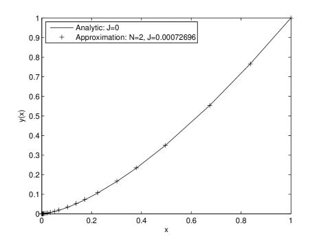
Figure 10.1: Analytic versus numerical solution to problem of Example 72.

This numerical method works well, even in the case the minimizer is not a Lipschitz function.

Example 97.

An approximated solution to the problem considered in Example 73 can be obtained following exactly the same steps as in Example 96. Recall that the minimizer (10.8) to that problem is not a Lipschitz function. As before, one has $x(0)=0$ and the Caputo derivative coincides with the Riemann–Liouville derivative. We approximate the fractional problem using (5.10). Let ${}^{C}_{0}D_{t}^{\alpha}x(t)=u(t)$. Then (10.36) holds. In this case the variable $z(t)$ satisfies

$$\dot{z}(t)=\left(x(t)-\frac{t^{\alpha}}{\Gamma(\alpha+1)}\right)^{2},$$

and we approximate the fractional variational problem with the following classical one:

$$\begin{gathered}\tilde{J}[x]=\int_{0}^{1}\left[(u(t)-1)^{2}+z(t)\right]dt\longrightarrow\min\\ \begin{cases}\dot{x}(t)=-AB^{-1}t^{-1}x(t)+\sum_{k=2}^{N}B^{-1}C_{k}t^{-k}v_{k}(t)+B^{-1}t^{\alpha-1}u(t)\\ \dot{v}_{k}(t)=(1-k)t^{k-2}x(t),\qquad k=1,2,\ldots\\ \displaystyle\dot{z}(t)=\left(x(t)-\frac{t^{\alpha}}{\Gamma(\alpha+1)}\right)^{2},\end{cases}\end{gathered}$$

subject to the boundary conditions $x(0)=0$, $z(0)=0$ and $v_{k}(0)=0$, $k=1,2,\ldots$ Setting $N=2$, the Hamiltonian is given by

$$H=-[(u(t)-1)^{2}+z(t)]+p_{1}(t)\left(-AB^{-1}t^{-1}x(t)+B^{-1}C_{2}t^{-2}v_{2}(t)+B^{-1}t^{\alpha-1}u(t)\right)\\ -p_{2}(t)x(t)+p_{3}(t)\left(x(t)-\frac{t^{\alpha}}{\Gamma(\alpha+1)}\right)^{2}.$$

The classical theory [94] tells us to solve the system

$$\left\{\begin{array}[]{ll}\dot{x}(t)&=-AB^{-1}t^{-1}x(t)+B^{-1}C_{2}t^{-2}v_{2}(t)+\displaystyle\frac{1}{2}B^{-2}t^{2\alpha-2}p_{1}(t)+B^{-1}t^{\alpha-1}\\[5.0pt] \dot{v}_{2}(t)&=-x(t)\\[5.0pt] \dot{z}(t)&=\left(x(t)-\displaystyle\frac{t^{\alpha}}{\Gamma(\alpha+1)}\right)^{2}\\[5.0pt] \dot{p}_{1}(t)&=AB^{-1}t^{-1}p_{1}(t)+p_{2}(t)-2p_{3}(t)\left(x(t)-\displaystyle\frac{t^{\alpha}}{\Gamma(\alpha+1)}\right)\\ \dot{p}_{2}(t)&=-B^{-1}C_{2}t^{-2}p_{1}(t)\\ \dot{p}_{3}(t)&=1,\end{array}\right.$$ (10.40)

subject to boundary conditions

$$\begin{cases}x(0)=0\\ v_{2}(0)=0\\ z(0)=0\end{cases},\qquad\begin{cases}\displaystyle x(1)=\frac{1}{\Gamma(\alpha+1)}\\ p_{2}(1)=0\\ p_{3}(1)=0.\end{cases}$$ (10.41)

As done in Example 96, we solved (10.40)–(10.41) using the MATLAB^® built-in function bvp4c. The resulting graph for $x(t)$, together with the corresponding value of $J$, is given in Figure 10.2 in contrast with the exact minimizer (10.8).

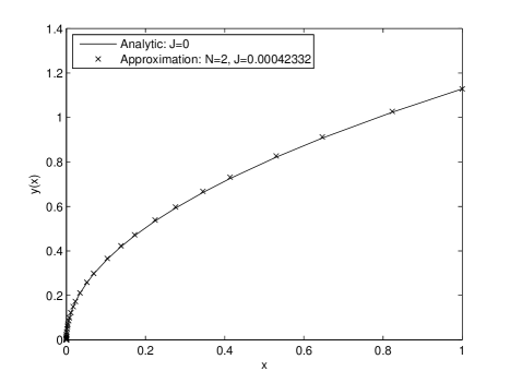
Figure 10.2: Analytic versus numerical solution to problem of Example 73.

Conclusion and future work

The realm of numerical methods in scientific fields is vastly growing due to the very fast progresses in computational sciences and technologies. Nevertheless, the intrinsic complexity of fractional calculus, caused partially by non-local properties of fractional derivatives and integrals, makes it rather difficult to find efficient numerical methods in this field. It seems enough to mention here that, up to the time of this thesis and to the best of our knowledge, there is no routine available for solving a fractional differential equation as Runge–Kutta for ordinary ones. Despite this fact, however, the literature exhibits a growing interest and improving achievements in numerical methods for fractional calculus in general and fractional variational problems specifically.

This thesis is devoted to discussing some aspects of the very well-known methods for solving variational problems. Namely, we studied the notions of direct and indirect methods in the classical calculus of variation and also we mentioned some connections to optimal control. Consequently, we introduced the generalizations of these notions to the field of fractional calculus of variations and fractional optimal control.

The method of finite differences, as discussed here, seems to be a potential first candidate to solve fractional variational problems. Although a first order approximation was used for all examples, the results are satisfactory and even though it is more complicated than in the classical case, it still inherits some sort of simplicity and an ease of implementation.

The outcomes of our works related to direct methods are as follows:

• S. Pooseh, R. Almeida and D. F. M. Torres, Discrete Direct Methods in the Fractional Calculus of Variations, Proceedings of FDA’2012, May 14-17, 2012, Hohai University, Nanjing, China. Paper #042, Winner of a best oral presentation award [96];

• S. Pooseh, R. Almeida and D.F.M. Torres, Discrete direct methods in the fractional calculus of variations, Comput. Math. Appl.,66 (2013), no. 5, 668–676 [99];

• S. Pooseh, R. Almeida and D. F. M. Torres, A discrete time method to the first variation of fractional order variational functionals, Cent. Eur. J. Phys, in press [103].

Roughly speaking, an Euler-like direct method reduces a variational problem to the solution of a system of algebraic equations. When the system is linear, we can freely increase the number of mesh points, $n$, and obtain better solutions as long as the resulted matrix of coefficients is invertible. The method is very fast, in this case, and the execution time is of order $10^{-4}$ for Examples 50 and 51. It is worth, however, to keep in mind that the Grünwald–Letnikov approximation is of first order, $\mathcal{O}(h)$, and even a large $n$ cannot result in a high precision. Actually, by increasing $n$, the solution slowly converges and in Example 51, a grid of $30$ points has the same order of error, $10^{-3}$, as a $5$ points grid. The situation is completely different when the problem ends with a nonlinear system. In Example 52, a small number of mesh points, $n=5$, results in a poor solution with the error $E=1.4787$. The MATLAB^® built in function fsolve takes $0.0126$ seconds to solve the problem. As one increases the number of mesh points, the solution gets closer to the analytic solution and the required time increases drastically. Finally, by $n=90$ we have $E=0.0618$ and the time is $T=26.355$ seconds.

In practice, we have no idea about the solution in advance and the worst case should be taken into account. Comparing the results of the three examples considered, reveals that for a typical fractional variational problem, the Euler-like direct method needs a large number of mesh points and most likely a long running time.

The lack of efficient numerical methods for fractional variational problems, is overcome partially by the indirect methods of this thesis. Once we transformed the fractional variational problem to an approximated classical one, the majority of classical methods can be applied to get an approximate solution. Nevertheless, the procedure is not completely straightforward. The singularity of fractional operators is still present in the approximating formulas and it makes the solution procedure more complicated.

During the last three decades, several numerical methods have been developed in the field of fractional calculus. Some of their advantages, disadvantages, and improvements, are given in [19]. Based on two continuous expansion formulas (5.2) and (5.7) for the left Riemann–Liouville fractional derivative, we studied two approximations (5.4) and (5.10) and their applications in the computation of fractional derivatives. Despite the fact that the approximation (5.4) encounters some difficulties from the presence of higher-order derivatives, it exhibits better results at least for the evaluation of fractional derivatives. The same studies were carried out for fractional integrals as well as some other fractional operators, namely Hadamard derivatives and integrals, and Caputo derivatives.

The full details regarding these approximations and their advantages, disadvantages and applications can be found in the following papers:

• S. Pooseh, R. Almeida and D. F. M. Torres, Numerical approximations of fractional derivatives with applications, Asian Journal of Control 15 (2013), no. 3, 698–712 [98];

• S. Pooseh, R. Almeida and D. F. M. Torres, Approximation of fractional integrals by means of derivatives, Comput. Math. Appl. 64 (2012), no. 10, 3090–3100 [95];

• S. Pooseh, R. Almeida and D.F.M. Torres, Expansion formulas in terms of integer-order derivatives for the Hadamard fractional integral and derivative, Numerical Functional Analysis and Optimization 33 (2012) No 3, 301–319 [97].

Approximation (5.10) can also be generalized to include higher-order derivatives in the form of (5.15). The possibility of using (5.10) to compute fractional derivatives for a set of tabular data was discussed. Fractional differential equations are also treated successfully. In this case the lack of initial conditions makes (5.4) less useful. In contrast, one can freely increase $N$, the order of approximation (5.10), and find better approximations. Comparing with (5.13), our modification provides better results.

For fractional variational problems, the proposed expansions may be used at two different stages during the solution procedure. The first approach, the one considered in Chapter 8, consists in a direct approximation of the problem, and then treating it as a classical problem, using standard methods to solve it. The second approach, Section 9.4.1, is to apply the fractional Euler–Lagrange equation and then to use the approximations in order to obtain a classical differential equation.

The results concerning the application of the approximations proposed in this work have been published as follows:

• R. Almeida, S. Pooseh and D. F. M. Torres, Fractional variational problems depending on indefinite integrals, Nonlinear Anal. 75 (2012), no. 3, 1009–1025 [12];

• S. Pooseh, R. Almeida and D. F. M. Torres, Fractional order optimal control problems with free terminal time, J. Ind. Manag. Optim. 10 (2014), no. 2, 363–381 [102];

• S. Pooseh, R. Almeida and D. F. M. Torres, Free fractional optimal control problems, 2013 European Control Conference (ECC) July 17-19, 2013, Zurich, Switzerland [101].

• S. Pooseh, R. Almeida and D. F. M. Torres, A numerical scheme to solve fractional optimal control problems, Conference Papers in Mathematics, vol. 2013, Article ID 165298, 10 pages, 2013 [100].

The direct methods for fractional variational problems presented in this thesis, can be improved in some stages. One can try different approximations for the fractional derivative that exhibit higher order precisions, e.g. Diethelm’s backward finite differences [41]. Better quadrature rules can be applied to discretize the functional and, finally, we can apply more sophisticated algorithms for solving the resulting system of algebraic equations. Further works are needed to cover different types of fractional variational problems.

Regarding indirect methods, the idea of transforming a fractional problem to a classic one seems a useful way of extending the available classic methods to the field of fractional variational problems. Nevertheless, improvements are needed to avoid the singularities of the approximations (5.10) and (5.4). A more practical goal is to implement some software packages or tools to solve certain classes of fractional variational problems. Following this research direction may also end in some solvers for fractional differential equations.

In the course of this thesis we have also studied the use of fractional calculus in epidemiology, that is not included in this thesis [104]. The proposed approach is illustrated with an outbreak of dengue disease, which is motivated by the first dengue epidemic ever recorded in the Cape Verde islands off the coast of west Africa, in 2009. Describing the reality through a mathematical model, usually a system of differential equations, is a hard task that has an inherent compromise between simplicity and accuracy. In our work, we consider a very basic model to dengue epidemics. It turns out that, in general, this basic/classical model does not provide enough good results. In order to have better results, that fit the reality, more specific and complicated set of differential equations have been investigated in the literature, see [108, 109, 110] and references therein. We have proposed a completely new approach to the subject. We keep the simple model and substitute the usual (local) derivatives by (non-local) fractional differentiation. The use of fractional derivatives allow us to model memory effects, and result in a more powerful approach to epidemiological models: one can then design the order $\alpha$ of fractional differentiation that best corresponds to reality. The classical case is recovered by taking the limit when $\alpha$ goes to one. Our investigations show that even a simple fractional model may give surprisingly good results [104]. However, the transformation of a classical model into a fractional one makes it very sensitive to the order of differentiation $\alpha$: a small change in $\alpha$ may result in a big change in the final result. This work was presented at ICNAAM 2011, Numerical Optimization and Applications Symposium:

• S. Pooseh, H. S. Rodrigues and D. F. M. Torres, Fractional Derivatives in Dengue Epidemics, Numerical Analysis and Applied Mathematics ICNAAM 2011, AIP Conf. Proc. 1389, 739–742 (2011) [104],

and a more sophisticated study has been reported in [39].

Our work can be extended in several ways: by fractionalizing more sophisticated models; by considering different orders of fractional derivatives for each one of the state variables, i.e., models of non-commensurate order. Finally, we can combine the results of this PhD thesis in the framework of fractional optimal control of epidemic models.

References

- [1] O. P. Agrawal, Formulation of Euler-Lagrange equations for fractional variational problems, J. Math. Anal. Appl. 272 (2002), no. 1, 368–379.
- [2] O. P. Agrawal, A general formulation and solution scheme for fractional optimal control problems, Nonlinear Dynam. 38 (2004), no. 1-4, 323–337.
- [3] O. P. Agrawal, Fractional variational calculus in terms of Riesz fractional derivatives, J. Phys. A 40 (2007), no. 24, 6287–6303.
- [4] O. P. Agrawal, Generalized Euler-Lagrange equations and transversality conditions for FVPs in terms of the Caputo derivative, J. Vib. Control 13 (2007), no. 9-10, 1217–1237.
- [5] O. P. Agrawal, A formulation and numerical scheme for fractional optimal control problems, J. Vib. Control 14 (2008), no. 9-10, 1291–1299.
- [6] O. P. Agrawal, A general finite element formulation for fractional variational problems, J. Math. Anal. Appl. 337 (2008), no. 1, 1–12.
- [7] O. P. Agrawal, O. Defterli and D. Baleanu, Fractional optimal control problems with several state and control variables, J. Vib. Control 16 (2010), no. 13, 1967–1976.
- [8] O. P. Agrawal, S. I. Muslih and D. Baleanu, Generalized variational calculus in terms of multi-parameters fractional derivatives, Commun. Nonlinear Sci. Numer. Simul. 16 (2011), no. 12, 4756–4767.
- [9] R. Almeida, R. A. C. Ferreira and D. F. M. Torres, Isoperimetric problems of the calculus of variations with fractional derivatives, Acta Math. Sci. Ser. B Engl. Ed. 32 (2012), no. 2, 619–630. arXiv:1105.2078
- [10] R. Almeida, A. B. Malinowska and D. F. M. Torres, A fractional calculus of variations for multiple integrals with application to vibrating string, J. Math. Phys. 51 (2010), no. 3, 033503, 12 pp. arXiv:1001.2722
- [11] R. Almeida, A. B. Malinowska and D. F. M. Torres, Fractional Euler-Lagrange differential equations via Caputo derivatives, in Fractional Dynamics and Control (eds: D. Baleanu, J. A. Tenreiro Machado, and A. Luo), Springer New York, 2012, Part 2, 109–118. arXiv:1109.0658
- [12] R. Almeida, S. Pooseh and D. F. M. Torres, Fractional variational problems depending on indefinite integrals, Nonlinear Anal. 75 (2012), no. 3, 1009–1025. arXiv:1102.3360
- [13] R. Almeida and D. F. M. Torres, Calculus of variations with fractional derivatives and fractional integrals, Appl. Math. Lett. 22 (2009), no. 12, 1816–1820. arXiv:0907.1024
- [14] R. Almeida and D. F. M. Torres, Hölderian variational problems subject to integral constraints, J. Math. Anal. Appl. 359 (2009), no. 2, 674–681. arXiv:0807.3076
- [15] R. Almeida and D. F. M. Torres, Isoperimetric problems on time scales with nabla derivatives, J. Vib. Control 15 (2009), no. 6, 951–958. arXiv:0811.3650
- [16] R. Almeida and D. F. M. Torres, Leitmann’s direct method for fractional optimization problems, Appl. Math. Comput. 217 (2010), no 3, 956–962. arXiv:1003.3088
- [17] R. Almeida and D. F. M. Torres, Necessary and sufficient conditions for the fractional calculus of variations with Caputo derivatives, Commun. Nonlinear Sci. Numer. Simulat. 16 (2011), no. 3, 1490–1500. arXiv:1007.2937
- [18] G. E. Andrews, R. Askey and R. Roy, Special functions, Encyclopedia of Mathematics and its Applications, 71, Cambridge Univ. Press, Cambridge, 1999.
- [19] M. Aoun, R. Malti, F. Levron and A. Oustaloup, Numerical simulations of fractional systems: An overview of existing methods and improvements, Nonlinear Dynam. 38 (2004), no. 1-4, 117–131.
- [20] T. M. Atanacković, S. Konjik, Lj. Oparnica and S. Pilipović, Generalized Hamilton’s principle with fractional derivatives, J. Phys. A 43 (2010), no. 25, 255203, 12 pp.
- [21] T. M. Atanacković, S. Konjik and S. Pilipović, Variational problems with fractional derivatives: Euler-Lagrange equations, J. Phys. A 41 (2008), no. 9, 095201, 12 pp. arXiv:1101.2961
- [22] T. M. Atanacković and B. Stanković, An expansion formula for fractional derivatives and its application, Fract. Calc. Appl. Anal. 7 (2004), no. 3, 365–378.
- [23] T. M. Atanacković and B. Stanković, On a numerical scheme for solving differential equations of fractional order, Mech. Res. Comm. 35 (2008), no. 7, 429–438.
- [24] S. N. Avvakumov and Yu. N. Kiselev, Boundary value problem for ordinary differential equations with applications to optimal control, in Spectral and evolution problems, Vol. 10 (Sevastopol, 1999), 147–155, Natl. Taurida Univ. “V. Vernadsky”, Simferopol, 2000.
- [25] D. Baleanu, O. Defterli and O. P. Agrawal, A central difference numerical scheme for fractional optimal control problems, J. Vib. Control 15 (2009), no. 4, 583–597.
- [26] D. Baleanu, K. Diethelm, E. Scalas and J. J. Trujillo, Fractional calculus, Series on Complexity, Nonlinearity and Chaos, 3, World Scientific Publishing Co. Pte. Ltd., Hackensack, NJ, 2012.
- [27] N. R. O. Bastos, R. A. C. Ferreira and D. F. M. Torres, Discrete-time fractional variational problems, Signal Processing 91 (2011), no. 3, 513–524. arXiv:1005.0252
- [28] R. Beals and R. Wong, Special functions, Cambridge Studies in Advanced Mathematics, 126, Cambridge Univ. Press, Cambridge, 2010.
- [29] V. L. Berdichevsky, Variational principles of continuum mechanics. II, Interaction of Mechanics and Mathematics, Springer, Berlin, 2009.
- [30] S. Bhalekar, V. Daftardar-Gejji, D. Baleanu and R. Magin, Generalized fractional order bloch equation with extended delay, Internat. J. Bifur. Chaos Appl. Sci. Engrg. 22 (2012), no. 4, 1250071, 15 pp.
- [31] S. Bhalekar, V. Daftardar-Gejji, D. Baleanu and R. Magin, Transient chaos in fractional Bloch equations, Comput. Math. Appl. 64 (2012), no. 10, 3367–3376.
- [32] A. M. C. Brito da Cruz, N. Martins and D. F. M. Torres, Higher-order Hahn’s quantum variational calculus, Nonlinear Anal. 75 (2012), no. 3, 1147–1157. arXiv:1101.3653
- [33] A. E. Bryson, Jr. and Y. C. Ho, Applied optimal control, Hemisphere Publishing Corp. Washington, DC, 1975.
- [34] P. L. Butzer, A. A. Kilbas and J. J. Trujillo, Mellin transform analysis and integration by parts for Hadamard-type fractional integrals, J. Math. Anal. Appl. 270 (2002), no. 1, 1–15.
- [35] P. L. Butzer, A. A. Kilbas and J. J. Trujillo, Stirling functions of the second kind in the setting of difference and fractional calculus, Numer. Funct. Anal. Optim. 24 (2003), no. 7-8, 673–711.
- [36] A. C. Chiang, Elements of Dynamic Optimization, McGraw-Hill Inc., Singapore, 1992.
- [37] S. Das, Functional fractional calculus for system identification and controls, Springer, Berlin, 2008.
- [38] K. Diethelm, The analysis of fractional differential equations, Lecture Notes in Mathematics, 2004, Springer, Berlin, 2010.
- [39] K. Diethelm, A fractional calculus based model for the simulation of an outbreak of dengue fever, Nonlinear Dyn. 71 (2013), no. 4, 613–619.
- [40] K. Diethelm, N. J. Ford and A. D. Freed, A predictor-corrector approach for the numerical solution of fractional differential equations, Nonlinear Dynam. 29 (2002), no. 1-4, 3–22.
- [41] K. Diethelm, N. J. Ford, A. D. Freed and Yu. Luchko, Algorithms for the fractional calculus: a selection of numerical methods, Comput. Methods Appl. Mech. Engrg. 194 (2005), no. 6-8, 743–773.
- [42] V. D. Djordjevic and T. M. Atanackovic, Similarity solutions to nonlinear heat conduction and Burgers/Korteweg-de Vries fractional equations, J. Comput. Appl. Math. 222 (2008), no. 2, 701–714.
- [43] M. Ö. Efe, Battery power loss compensated fractional order sliding mode control of a quadrotor UAV, Asian J. Control 14 (2012), no. 2, 413–425.
- [44] R. A. El-Nabulsi and D. F. M. Torres, Necessary optimality conditions for fractional action-like integrals of variational calculus with Riemann-Liouville derivatives of order , Math. Methods Appl. Sci. 30 (2007), no. 15, 1931–1939. arXiv:math-ph/0702099
- [45] R. A. El-Nabulsi and D. F. M. Torres, Fractional actionlike variational problems, J. Math. Phys. 49 (2008), no. 5, 053521, 7 pp. arXiv:0804.4500
- [46] L. Elsgolts, Differential equations and the calculus of variations, translated from the Russian by George Yankovsky, Mir Publishers, Moscow, 1973.
- [47] R. A. C. Ferreira and D. F. M. Torres, Higher-order calculus of variations on time scales, in Mathematical control theory and finance (eds: A. Sarychev, A. Shiryaev, M. Guerra, and M. do R. Grossinho), 149–159, Springer, Berlin, 2008. arXiv:0706.3141
- [48] R. A. C. Ferreira and D. F. M. Torres, Isoperimetric problems of the calculus of variations on time scales, in Nonlinear Analysis and Optimization II (eds: A. Leizarowitz, B. S. Mordukhovich, I. Shafrir, and A. J. Zaslavski), Contemporary Mathematics, vol. 514, Amer. Math. Soc., Providence, RI, 2010, 123–131. arXiv:0805.0278
- [49] R. A. C. Ferreira and D. F. M. Torres, Fractional -difference equations arising from the calculus of variations, Appl. Anal. Discrete Math. 5 (2011), no. 1, 110–121. arXiv:1101.5904
- [50] N. J. Ford and J. A. Connolly, Comparison of numerical methods for fractional differential equations, Commun. Pure Appl. Anal. 5 (2006), no. 2, 289–306.
- [51] C. G. Fraser, Isoperimetric problems in the variational calculus of Euler and Lagrange, Historia Math. 19 (1992), no. 1, 4–23.
- [52] G. S. F. Frederico and D. F. M. Torres, A formulation of Noether’s theorem for fractional problems of the calculus of variations, J. Math. Anal. Appl. 334 (2007), no. 2, 834–846. arXiv:math/0701187
- [53] G. S. F. Frederico and D. F. M. Torres, Fractional conservation laws in optimal control theory, Nonlinear Dynam. 53 (2008), no. 3, 215–222. arXiv:0711.0609
- [54] G. S. F. Frederico and D. F. M. Torres, Fractional optimal control in the sense of Caputo and the fractional Noether’s theorem, Int. Math. Forum 3 (2008), no. 10, 479–493. arXiv:0712.1844
- [55] G. S. F. Frederico and D. F. M. Torres, Fractional Noether’s theorem in the Riesz-Caputo sense, Appl. Math. Comput. 217 (2010), no. 3, 1023–1033. arXiv:1001.4507
- [56] H. H. Goldstine, A history of the calculus of variations from the 17th through the 19th century, Studies in the History of Mathematics and Physical Sciences, 5, Springer, New York, 1980.
- [57] P. D. F. Gouveia, A. Plakhov and D. F. M. Torres, Two-dimensional body of maximum mean resistance, Appl. Math. Comput. 215 (2009), no. 1, 37–52. arXiv:0904.2781
- [58] J. Gregory, Generalizing variational theory to include the indefinite integral, higher derivatives, and a variety of means as cost variables, Methods Appl. Anal. 15 (2008), no. 4, 427–435.
- [59] J. Gregory and C. Lin, Discrete variable methods for the -dependent variable nonlinear, extremal problem in the calculus of variations. II, SIAM J. Numer. Anal. 30 (1993), no. 3, 871–881.
- [60] J. Gregory and R. S. Wang, Discrete variable methods for the -dependent variable, nonlinear extremal problem in the calculus of variations, SIAM J. Numer. Anal. 27 (1990), no. 2, 470–487.
- [61] J. Hadamard, Essai sur l’étude des fonctions données par leur développement de Taylor, Journ. de Math. 4 (1892), no. 8, 101–186.
- [62] F. Jarad, T. Abdeljawad and D. Baleanu, Stability of -fractional non-autonomous systems, Nonlinear Anal. Real World Appl. 14 (2013), no. 1, 780–784.
- [63] Z. D. Jelicic and N. Petrovacki, Optimality conditions and a solution scheme for fractional optimal control problems, Struct. Multidiscip. Optim. 38 (2009), no. 6, 571–581.
- [64] U. N. Katugampola, New approach to a generalized fractional integral, Appl. Math. Comput. 218 (2011), no. 3, 860–865.
- [65] A. A. Kilbas, Hadamard-type fractional calculus, J. Korean Math. Soc. 38 (2001), no. 6, 1191–1204.
- [66] A. A. Kilbas, H. M. Srivastava and J. J. Trujillo, Theory and applications of fractional differential equations, North-Holland Mathematics Studies, 204, Elsevier, Amsterdam, 2006.
- [67] A. A. Kilbas and A. A. Titioura, Nonlinear differential equations with Marchaud-Hadamard-type fractional derivative in the weighted space of summable functions, Math. Model. Anal. 12 (2007), no. 3, 343–356.
- [68] D. E. Kirk, Optimal control theory: An introduction, North-Holland Mathematics Studies, 204, Prentice-Hall Inc., Englewood Cliffs, NJ, 1970.
- [69] M. Klimek, Fractional sequential mechanics—models with symmetric fractional derivative, Czechoslovak J. Phys. 51 (2001), no. 12, 1348–1354.
- [70] P. Kumar and O. P. Agrawal, An approximate method for numerical solution of fractional differential equations, Signal Process. 86 (2006), 2602–2610.
- [71] L. P. Lebedev and M. J. Cloud, The calculus of variations and functional analysis, World Sci. Publishing, River Edge, NJ, 2003.
- [72] Y. Li, Y. Chen and H.-S. Ahn, Fractional-order iterative learning control for fractional-order linear systems, Asian J. Control 13 (2011), no. 1, 54–63.
- [73] Q. Lin, R. Loxton, K. L. Teo and Y. H. Wu, A new computational method for a class of free terminal time optimal control problems, Pac. J. Optim. 7 (2011), no. 1, 63–81.
- [74] Q. Lin, R. Loxton, K. L. Teo and Y. H. Wu, Optimal control computation for nonlinear systems with state-dependent stopping criteria, Automatica J. IFAC 48 (2012), no. 9, 2116–2129.
- [75] A. Lotfi and M. Dehghan and S.A. Yousefi, A numerical technique for solving fractional optimal control problems, Comput. Math. Appl. 59 (2011), 1055–1067.
- [76] A. B. Malinowska and D. F. M. Torres, Delta-nabla isoperimetric problems, Int. J. Open Probl. Comput. Sci. Math. 3 (2010), no. 4, 124–137. arXiv:1010.2956
- [77] A. B. Malinowska and D. F. M. Torres, Generalized natural boundary conditions for fractional variational problems in terms of the Caputo derivative, Comput. Math. Appl. 59 (2010), no. 9, 3110–3116. arXiv:1002.3790
- [78] A. B. Malinowska and D. F. M. Torres, Natural boundary conditions in the calculus of variations, Math. Methods Appl. Sci. 33 (2010), no. 14, 1712–1722. arXiv:0812.0705
- [79] A. B. Malinowska and D. F. M. Torres, Introduction to the fractional calculus of variations, Imp. Coll. Press, London, 2012.
- [80] N. Martins and D. F. M. Torres, Calculus of variations on time scales with nabla derivatives, Nonlinear Anal. 71 (2009), no. 12, e763–e773. arXiv:0807.2596
- [81] N. Martins and D. F. M. Torres, Generalizing the variational theory on time scales to include the delta indefinite integral, Comput. Math. Appl. 61 (2011), no. 9, 2424–2435. arXiv:1102.3727
- [82] M. M. Meerschaert and C. Tadjeran, Finite difference approximations for fractional advection-dispersion flow equations, J. Comput. Appl. Math. 172 (2004), no. 1, 65–77.
- [83] K. S. Miller and B. Ross, An introduction to the fractional calculus and fractional differential equations, A Wiley-Interscience Publication, Wiley, New York, 1993.
- [84] D. Mozyrska and D. F. M. Torres, Minimal modified energy control for fractional linear control systems with the Caputo derivative, Carpathian J. Math. 26 (2010), no. 2, 210–221. arXiv:1004.3113
- [85] D. Mozyrska and D. F. M. Torres, Modified optimal energy and initial memory of fractional continuous-time linear systems, Signal Process. 91 (2011), no. 3, 379–385. arXiv:1007.3946
- [86] T. Odzijewicz, A. B. Malinowska and D. F. M. Torres, Fractional calculus of variations in terms of a generalized fractional integral with applications to physics, Abstr. Appl. Anal. 2012 (2012), Art. ID 871912, 24 pp. arXiv:1203.1961
- [87] T. Odzijewicz, A. B. Malinowska and D. F. M. Torres, Fractional variational calculus with classical and combined Caputo derivatives, Nonlinear Anal. 75 (2012), no. 3, 1507–1515. arXiv:1101.2932
- [88] T. Odzijewicz and D. F. M. Torres, Fractional calculus of variations for double integrals, Balkan J. Geom. Appl. 16 (2011), no. 2, 102–113. arXiv:1102.1337
- [89] M. D. Ortigueira, Fractional calculus for scientists and engineers, Lecture Notes in Electrical Engineering, 84, Springer, Dordrecht, 2011.
- [90] M. D. Ortigueira and F. V. Coito, The initial conditions of Riemann-Liouville and Caputo derivatives, in: Proceedings of the Sixth EUROMECH Conference ENOC 2008, June 30-July 4, 2008, Saint Petersburg, Russia.
- [91] M. D. Ortigueira and F. V. Coito, On the usefulness of Riemann-Liouville and Caputo derivatives in describing fractional shift-invariant linear systems, Journal of Applied Nonlinear Dynamics 1 (2012), no. 2, 113–124.
- [92] A. Yu. Plakhov and D. F. M. Torres, Newton’s aerodynamic problem in a medium consisting of moving particles, Mat. Sb. 196 (2005), no. 6, 111–160; translation in Sb. Math. 196 (2005), no. 5-6, 885–933. arXiv:math/0407406
- [93] I. Podlubny, Fractional differential equations, Mathematics in Science and Engineering, 198, Academic Press, San Diego, CA, 1999.
- [94] L. S. Pontryagin, V. G. Boltyanskii, R. V. Gamkrelidze and E. F. Mishchenko, The mathematical theory of optimal processes, Translated from the Russian by K. N. Trirogoff; edited by L. W. Neustadt, Interscience Publishers John Wiley & Sons Inc., New York, 1962.
- [95] S. Pooseh, R. Almeida and D. F. M. Torres, Approximation of fractional integrals by means of derivatives, Comput. Math. Appl. 64 (2012), no. 10, 3090–3100. arXiv:1201.5224
- [96] S. Pooseh, R. Almeida and D. F. M. Torres, Discrete direct methods in the fractional calculus of variations, Proceedings of FDA’2012, May 14-17, 2012, Hohai University, Nanjing, China. Paper #042 arXiv:1205.4843
- [97] S. Pooseh, R. Almeida and D. F. M. Torres, Expansion formulas in terms of integer-order derivatives for the Hadamard fractional integral and derivative, Numer. Funct. Anal. Optim. 33 (2012), no. 3, 301–319. arXiv:1112.0693
- [98] S. Pooseh, R. Almeida and D. F. M. Torres, Numerical approximations of fractional derivatives with applications, Asian J. Control 15 (2013), no. 3, 698–712. arXiv:1208.2588
- [99] S. Pooseh, R. Almeida and D. F. M. Torres, Discrete direct methods in the fractional calculus of variations, Comput. Math. Appl. 66 (2013), no. 5, 668–676. arXiv:1205.4843
- [100] S. Pooseh, R. Almeida and D. F. M. Torres, A numerical scheme to solve fractional optimal control problems, Conference Papers in Mathematics 2013 (2013), Art. ID 165298, 10 pp. arXiv:1306.0203
- [101] S. Pooseh, R. Almeida and D. F. M. Torres, Free time fractional optimal control problems, Proceedings of the European Control Conference 2013, Zurich, Switzerland, July 17-19, 2013, 3985–3990.
- [102] S. Pooseh, R. Almeida and D. F. M. Torres, Fractional order optimal control problems with free terminal time, J. Ind. Manag. Optim. 10 (2014), no. 2, 363–381. arXiv:1302.1717
- [103] S. Pooseh, R. Almeida and D. F. M. Torres, A discrete time method to the first variation of fractional order variational functionals, Cent. Eur. J. Phys., in press. DOI:10.2478/s11534-013-0250-0 arXiv:1305.1859
- [104] S. Pooseh, H. S. Rodrigues and D. F. M. Torres, Fractional derivatives in dengue epidemics, Numerical Analysis and Applied Mathematics ICNAAM 2011, AIP Conf. Proc. 1389 (2011), no. 1, 739–742. arXiv:1108.1683
- [105] D. Qian, Z. Gong and C. Li, A generalized Gronwall inequality and its application to fractional differential equations with Hadamard derivatives, 3rd Conference on Nonlinear Science and Complexity (NSC10), Cankaya University, 1–4, Ankara, Turkey, 28–31 July, 2010.
- [106] F. Riewe, Nonconservative Lagrangian and Hamiltonian mechanics, Phys. Rev. E (3) 53 (1996), no. 2, 1890–1899.
- [107] F. Riewe, Mechanics with fractional derivatives, Phys. Rev. E (3) 55 (1997), no. 3, part B, 3581–3592.
- [108] H. S. Rodrigues, M. T. T. Monteiro and D. F. M. Torres, Dynamics of Dengue epidemics when using optimal control, Math. Comput. Modelling 52 (2010), 1667–1673. arXiv:1006.4392
- [109] H. S. Rodrigues, M. T. T. Monteiro and D. F. M. Torres, Insecticide control in a Dengue epidemics model, Numerical Analysis and Applied Mathematics, edited by T. Simos, AIP Conf. Proc. 1281 (2010), no. 1, 979–982. arXiv:1007.5159
- [110] H. S. Rodrigues, M. T. T. Monteiro, D. F. M. Torres and A. Zinober, Dengue disease, basic reproduction number and control, Int. J. Comput. Math. 89 (2012), no. 3, 334–346. arXiv:1103.1923
- [111] S. G. Samko, A. A. Kilbas and O. I. Marichev, Fractional integrals and derivatives, translated from the 1987 Russian original, Gordon and Breach, Yverdon, 1993.
- [112] J. Shen and J. Cao, Necessary and sufficient conditions for consensus of delayed fractional-order systems, Asian J. Control 14 (2012), no. 6, 1690–1697.
- [113] C. J. Silva and D. F. M. Torres, Two-dimensional Newton’s problem of minimal resistance, Control Cybernet. 35 (2006), no. 4, 965–975. arXiv:math/0607197
- [114] J. Stoer and R. Bulirsch, Introduction to numerical analysis, translated from the German by R. Bartels, W. Gautschi and C. Witzgall, third edition, Texts in Applied Mathematics, 12, Springer, New York, 2002.
- [115] W. Sun, Y. Li, C. Li and Y. Chen, Convergence speed of a fractional order consensus algorithm over undirected scale-free networks, Asian J. Control 13 (2011), no. 6, 936–946.
- [116] H. J. Sussmann and J. C. Willems, The brachistochrone problem and modern control theory, in Contemporary trends in nonlinear geometric control theory and its applications (México City, 2000), 113–166, World Sci. Publ., River Edge, NJ 2002.
- [117] J. A. Tenreiro Machado, V. Kiryakova and F. Mainardi, Recent history of fractional calculus, Commun. Nonlinear Sci. Numer. Simul. 16 (2011), no. 3, 1140–1153.
- [118] J. A. Tenreiro Machado, M. F. Silva, R. S. Barbosa, I. S. Jesus, C. M. Reis, M. G. Marcos and A. F. Galhano, Some applications of fractional calculus in engineering, Math. Probl. Eng., Art. ID 639801 (2010), 34 pp.
- [119] C. Tricaud and Y. Chen, An approximate method for numerically solving fractional order optimal control problems of general form, Comput. Math. Appl. 59 (2010), no. 5, 1644–1655.
- [120] C. Tricaud and Y. Chen, Time-optimal control of systems with fractional dynamics, Int. J. Differ. Equ. 2010, Art. ID 461048, 16 pp.
- [121] J. C. Trigeassou, N. Maamri and A. Oustaloup, The infinite state approach: Origin and necessity, Comput. Math. Appl. 66 (2013), no. 5, 892–907.
- [122] C. Tuckey, Nonstandard methods in the calculus of variations, Pitman Research Notes in Mathematics Series, 297, Longman Sci. Tech., Harlow, 1993.
- [123] B. van Brunt, The calculus of variations, Universitext, Springer, New York, 2004.
- [124] S. A. Yousefi, A. Lotfi and M. Dehghan, The use of a Legendre multiwavelet collocation method for solving the fractional optimal control problems, J. Vib. Control 17 (2011), no. 13, 2059–2065.
Index
- Binomial
- Boundary conditions §1.1.2, §10.4, §3.3
- Brachistochrone §1.1.1
-
Caputo fractional derivative
- Left Definition 14, Remark 24
- Right Definition 14, Remark 24
- Direct method §1.1.3, §1.2.1, §3.4, Chapter 7
- Error
- Euler method §1.1.3, §7.2.1
-