New approach to finding the maximum number of mutually unbiased bases in $\mathbb{C}^{6}$

Abstract

There has been great interest in finding sets of $m$ mutually unbiased bases which are compatible with a given space $\mathbb{C}^{d}$, specially in physics due to their interesting applications in quantum information theory. Several general results have been obtained so far, but surprising results may occur for definite $(m,d)$-values. One such case that has remained an open question (the simplest case) is the one regarding the existence of $m=4$ mutually orthogonal bases for $d=6$. In the present work we introduce a new approach to the problem by translating it into an optimization procedure for a given pair $(m,d)$.

I Introduction

The paradigm of observables defined on an infinite Hilbert space being mutually incompatible in quantum mechanics is provided by the Heisenberg commutation relations for the position and momentum operators. The associated Heisenberg group –in connection with the corresponding Weyl algebra– of phase-space translations is still relevant for systems with a finite number of orthogonal states, providing a basis of the space $\mathbb{C}^{d}$. As first studied by Schwinger, for each dimension $d\geq 2$ there is a set of unitary operators which give rise to a discrete equivalent of the Heisenberg-Weyl group schwinger60 .

We may somehow a priori expect that the kinematics of composite quantum systems will not depend on the dimensions of their building blocks. That is, that composite systems let us say consisting in the tensor product of two different Hilbert spaces (differing only in the corresponding dimensions) will undergo a similar evolution since they are structurally identical. Mathematically, the previous fact would imply the state spaces $\mathbb{C}^{d}$ to be structurally identical, at least with respect to properties closely related to the Heisenberg-Weyl group.

However, it is surprising that the aforementioned group allows one to construct $(d+1)$ so-called mutually unbiased (MU) bases of the space $\mathbb{C}^{d}$ if $d$ is the power of a prime number ivanovic81 ; wootters+89 , whereas the construction fails in all other dimensions. In point of fact, no other successful method to construct $(d+1)$ MU bases in all dimensions is known archer05 ; planat+06 .

Given $m=d+1$ orthonormal bases in the space $\mathbb{C}^{d}$, they are mutually unbiased if the moduli of the scalar products among the $d(d+1)$ basis vectors take these values:

$$\left|{\langle\psi_{j}^{b}|}{\psi_{j^{\prime}}^{b^{\prime}}\rangle}\right|=\left\{\begin{array}[]{ll}\delta_{jj^{\prime}}&\quad\mbox{if $b=b^{\prime}$}\,,\\ \frac{1}{\sqrt{d}}&\quad\mbox{if $b\neq b^{\prime}$}\,,\end{array}\right.$$ (1)

where $b,b^{\prime}=0,1,\ldots,d$. MU bases have useful applications in many quantum information processing. Such (complete) sets of MU bases are ideally suited to reconstruct quantum states wootters+89 while sets of up to $(d+1)$ MU bases have applications in quantum cryptography cerf+02 ; brierley09 and in the solution of the mean king’s problem aharonov+01 . Even for $d=6$, we do not know whether there exist four MU bases or not s6 ; s7 ; s8 ; s9 . Hence the research on the maximum number of bases for $d=6$ and construction of MU bases in $\mathbb{C}^{6}$ is of great importance. The issue of MU bases constitutes another part in the field of quantum information theory that is involved in pure mathematics, such as number theory, abstract algebra and projective algebra.

The methods to construct complete sets of MU bases typically deal with all prime or prime-power dimensions. They are constructive methods and effectively lead to the same bases. Two (or more) MU bases thus correspond to two (or more) unitary matrices, one of which can always be mapped to the identity $I$ of the space $\mathbb{C}^{d}$, using an overall unitary transformation. It then follows from the conditions (1) that the remaining unitary matrices must be complex Hadamard matrices: the moduli of all their matrix elements equal $1/\sqrt{d}$. This representation of MU bases links their classification to the classification of complex Hadamard matrices complex .

In this paper, we choose a different method to study MU bases in dimension six or any other dimension $d$. We will approach the problem by directly exploring the unitary matrices – randomly distributed, but according to the Haar measure – whose columns vectors constitute the bases elements, which must fulfill a series of requirements concerning their concomitant bases being unbiased. The overall scenario reduces to a simple –though a bit involved– optimization procedure. In point of fact, we shall perform a two-fold search employing i) an amoeba optimization procedure, where the optimal value is obtained at the risk of falling into a local minimum and ii) the so called simulated annealing kirkpatrick83 well-known search method, a Monte Carlo method, inspired by the cooling processes of molten metals. The advantage of this duplicity of computations is that we can be absolutely confident about the final result reached. Indeed, the second recipe contains a mechanism that allows a local search that eventually can escape from local optima.

This paper is organized as follows. In Section II we describe the generation of unitary matrices according to their natural Haar measure. Section III explains how the optimization is performed and the concomitant results are shown in Section IV. Finally, some conclusions are drawn in Section V.

II The Haar measure and the concomitant generation of ensembles of random matrices

The applications that have appeared so far in quantum information theory, in the form of dense coding, teleportation, quantum cryptography and specially in algorithms for quantum computing (quantum error correction codes for instance), deal with finite numbers of qubits. A quantum gate which acts upon these qubits or even the evolution of that system is represented by a unitary matrix $U(N)$, with $N=2^{n}$ being the dimension of the associated Hilbert space ${\cal H}_{N}$. The state $\rho$ describing a system of $n$ qubits is given by a hermitian, positive-semidefinite ($N\times N$) matrix, with unit trace. In view of these facts, it is natural to think that an interest has appeared in the quantification of certain properties of these systems, most of the times in the form of the characterization of a certain state $\rho$, described by $N\times N$ matrices of finite size. Natural applications arise when one tries to simulate certain processes through random matrices, whose probability distribution ought to be described accordingly.

This enterprise requires a quantitative measure $\mu$ on a given set of matrices. There is one natural candidate measure, the Haar measure on the group ${\cal U}(N)$ of unitary matrices. In mathematical analysis, the Haar measure Haar33 is known to assign an “invariant volume” to what is known as subsets of locally compact topological groups. Here we present the formal definition Conway90 : given a locally compact topological group $G$ (multiplication is the group operation), consider a $\sigma$-algebra $Y$ generated by all compact subsets of $G$. If $a$ is an element of $G$ and $S$ is a set in $Y$, then the set $aS=$ $\{$ $as:s\in S$ $\}$ also belongs to $Y$. A measure $\mu$ on $Y$ will be letf-invariant if $\mu(aS)=\mu(S)$ for all $a$ and $S$. Such an invariant measure is the Haar measure $\mu$ on $G$ (it happens to be both left and right invariant). In other words Haarsimetria , the Haar measure defines the unique invariant integration measure for Lie groups. It implies that a volume element d$\mu(g)$ is identified by defining the integral of a function $f$ over $G$ as $\int_{G}f(g)d\mu(g)$, being left and right invariant

$$\int_{G}f(g^{-1}x)d\mu(x)\,=\,\int_{G}f(xg^{-1})d\mu(x)\,=\,\int_{G}f(x)d\mu(x).$$ (2)

The invariance of the integral follows from the concomitant invariance of the volume element d$\mu(g)$. It is plain, then, that once d$\mu(g)$ is fixed at a given point, say the unit element $g=e$, we can move performing a left or right translation.

We do not gain much physical insight with these definitions of the Haar measure and its invariance, unless we identify $G$ with the group of unitary matrices ${\cal U}(N)$, the element $a$ with a unitary matrix $U$ and $S$ with subsets of the group of unitary matrices ${\cal U}(N)$, so that given a reference state $|\Psi_{0}\rangle$ and a unitary matrix $U\in{\cal U}(N)$, we can associate a state $|\Psi\rangle_{0}=U|\Psi_{0}\rangle$ to $|\Psi_{0}\rangle$. Physically what is required is a probability measure $\mu$ invariant under unitary changes of basis in the space of pure states, that is,

$$P^{(N)}_{Haar}(U\,|\Psi\rangle)\,=\,P^{(N)}_{Haar}(|\Psi\rangle).$$ (3)

These requirements can only be met by the Haar measure, which is rotationally invariant.

Now that we have justified what measure we need, we should be able to generate random matrices according to such a measure in arbitrary dimensions. The theory of random matrices Mehta90 specifies different ensembles of matrices, classified according to their different properties. In particular, the Circular Unitary Ensemble (CUE) consists of all matrices with the (normalized) Haar measure on the unitary group ${\cal U}(N)$. The Circular Orthogonal Ensemble (COE) is described in similar terms using orthogonal matrices, and it was useful in order to describe the entanglement features of two-rebits systems. Given a $N\times N$ unitary matrix $U$, the minimum number of independent entries is $N^{2}$. This number should match those elements that need to describe the Haar measure on ${\cal U}(N)$. This is best seen from the following reasoning. Suppose that a matrix $U$ is decomposed as a product of two (also unitary) matrices $U=XY$. In the vicinity of $Y$, we have Mehta90 $U+dU=X(1+idK)Y$, where $dK$ is a hermitian matrix with elements $dK_{ij}=dK^{R}_{ij}+idK^{I}_{ij}$. Then the probability measure nearby $dU$ is $P(dU)\sim\prod_{i\leq j}dK^{R}_{ij}\prod_{i<j}dK^{I}_{ij}$, which accounts for the number of independent variables. Such measure for CUE is invariant Mehta90 and therefore proportional to the Haar measure.

Yet, the aforementioned description is not useful for practical purposes. We need to parameterize the unitary matrices according to the Haar measure. According to the parameterization for CUE dating back to Hurwitz Hur1887 using Euler angles, the basic assumption is that an arbitrary unitary matrix can be decomposed into elementary two-dimensional transformations, denoted by $E^{i,j}(\phi,\psi,\chi)$:

$$E^{i,j}_{kk} = 1\,\,\,\,\,\,\,\,\,\,\,\,\,\,\,\,\,\,\,\,k=1,..,N;\,\,\,\,\,\,\,\,\,\,k\neq i,j$$ (4)

$$E^{i,j}_{ii} = \cos\phi\,e^{i\psi}$$ (5)

$$E^{i,j}_{ij} = \sin\phi\,e^{i\chi}$$ (6)

$$E^{i,j}_{ji} = -\sin\phi\,e^{-i\chi}$$ (7)

$$E^{i,j}_{jj} = \cos\phi\,e^{-i\psi}.$$ (8)

Using these elementary rotations we define the composite transformations

$$E_{1} = E^{N-1,N}(\phi_{01},\psi_{01},\chi_{1})$$ (9)

$$E_{2} = E^{N-2,N-1}(\phi_{12},\psi_{12},0)E^{N-1,N}(\phi_{02},\psi_{02},\chi_{2})$$ (10)

$$E_{3} = E^{N-3,N-2}(\phi_{23},\psi_{23},0)E^{N-2,N-1}(\phi_{13},\psi_{13},0)$$ (12)

$$E^{N-1,N}(\phi_{03},\psi_{03},\chi_{3})$$

$$... = ...$$ (13)

$$E_{N-1} = E^{1,2}(\phi_{N-2,N-1},\psi_{N-2,N-1},0)$$ (16)

$$E^{2,3}(\phi_{N-3,N-1},\psi_{N-3,N-1},0)...$$

$$E^{N-1,N}(\phi_{0,N-1},\psi_{0,N-1},\chi_{N-1}),$$

we finally form the matrix

$$U\,=\,e^{i\alpha}\,E_{1}E_{2}E_{3}...E_{N-1}$$ (17)

with the angles parameterizing the rotations

$$0\leq\phi_{rs}\leq\frac{\pi}{2}\,\,\,\,0\leq\psi_{rs}<2\pi\,\,\,\,0\leq\chi_{1s}<2\pi\,\,\,\,0\leq\alpha<2\pi.$$ (18)

The ensuing (normalized) Haar measure Girko90

$$P_{Haar}(dU)\, = \,\sqrt{N!2^{N(N-1)}}d\alpha$$ (21)

$$\prod_{1\leq r<s\leq N}\frac{1}{2r}d[(\sin\phi_{rs})^{2r}]d\psi_{rs}$$

$$\prod_{1<s\leq N}d\chi_{1s}$$

provides us with a random matrix belonging to CUE. Finally, we randomly generate the angles (18) uniformly and obtain the desired random matrix $U$ (17).

III Description of the optimization procedure

Let us formulate the problem of having $m$ orthonormal bases $B_{i},i=1..m$ in terms of the elements of a unitary matrix. All basis elements or vectors are obtained from a unitary matrix by identifying them with the corresponding columns. Unitarity guarantees that all vectors will therefore be orthonormal. Now we have to cope with the bases being unbiased amidst them. Since each basis is represented by a unitary matrix, we then have $B_{i},i=1..m\,\rightarrow\,U_{i},i=1..m$. This condition can be addressed by imposing that matrix elements

$$\big{(}U_{i}\cdot U_{j}\big{)}_{lm},$$ (22)

where $i=1<j\leq m$, have to be equal to $1/\sqrt{d}$. In other words, $U_{i}\cdot U_{j}$ has to be proportional to a Hadamard-like matrix. The aforementioned conditions has to be applied to all possible $m(m-1)/2$ bipartite combinations of bases $B_{i}$.

Let us define the following quantities as the residuals

$$\rho_{l,m,i,j}\equiv\bigg{(}\left|\big{(}U_{i}\cdot U_{j}\big{)}_{l,m}\right|^{2}\,-\,1/d\bigg{)}^{2}.$$ (23)

Thus, the problem of finding a set of unbiased orthonormal bases is translated into the optimization procedure of finding the minimum of $\sum_{l,m,i,j}\,\rho_{l,m,i,j}$ being equal to zero. If the minimum is different from zero, given $d$ and $m$, we definitely do not have a set of unbiased bases. In addition, our function resembles very much the quantity used in metrics to define the notion of “unbiasedness” between two orthonormal bases. To whether or not the aforementioned quantity represents a metric is something not checked.

Now that the we have translated the problem of finding MU bases into an operational one, one has to be able to explore all possible bases. This fact means that we have to be able to survey the set space of unitary matrices. Since we described in the previous section how to generate random unitary matrices properly, we will have to numerically explore all unitary matrices. The way to pursue that is to consider the angles (18) –given $d$ and $m$– in all cases in (22) as the variables of the function $\sum_{l,m,i,j}\,\rho_{l,m,i,j}$ to be minimized. Provided the concomitant optimal value (the sum of all residuals $\rho_{l,m,i,j}$) is equal to zero, we may then have found a set of MU bases. Otherwise, that may not be possible given the constraints on $d$ and $m$.

IV Results

Now that we have the tools to perform a numerical survey over the set of unitary matrices, we carry out the optimization described in the previous section.

IV.1 d=6, m=3

The $\mathbb{C}^{6}$ case with three bases is know to exist, so our numerical procedure must return a minimal value of zero. The results are depicted in Fig. (1). As can be appreciated, convergence is reached very fast after each Monte Carlo step (formed by 15000 different configurations each). Therefore, we are quite confident that we have found a set of MU bases in the $(d=6,m=3)-$case.

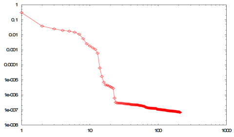
Figure 1: (Color online) Plot of the evolution of the sum of residuals –the figure of merit in the optimization– for the $d=6$ case with three basis vs. the number of Monte Carlo steps. As can be clearly appreciated, a global zero minimum is reached. See text for details.

However, we must bear in mind an important issue regarding numerical surveys. Not all our simulations lead to a zero minimum, so the lack of convergence is in favor of the argument that some sets of MU bases cannot be extended to further number of bases. In $d=6$ there are some sets of 2 MU bases that cannot be extended to 3 MU bases (see Ref. Dardo and references therein). From numerical simulations it is knows that null measure sets cannot be reached. In Dardo , a subset of the Karlson’s family of complex Hadamard matrices cannot be extended to 3 MU bases. Additionally, the Karlson’s family has dimension 2 and the maximal set of complex Hadamard matrices in dimension 6 has dimension 4, so it is a null measure set. Therefore, one could never achieve a unitary matrix from random simulations such that it belongs to the Karlsson’s family. Moreover, there are 1 dimensional families and even more, isolated complex Hadamard matrices in dimension six.

When considering the extension of the number of MU bases $\{I,H_{i}\}$, $H_{i}$ being a Hadamard matrix, provided by a certain number, we then know that that function lacks the property of continuity Jaming . The absence of continuity together with an incomplete knowledge about the number discontinuities in the number of MU bases makes the overall problem a difficult one. However, in our approach, we succeed in finding at least a few cases where $(m=3,d=6)$ holds.

The study of the case with three bases confirms that our approach to the problem is a good one. As a matter of fact, we could study the problem for any $(d,m)-$case, but the overall optimization procedure –as it is indeed the case for any simulation of a quantum system– becomes intractable at some point. With the numerical tools being a valid one, we can now tackle the problem of whether $\mathbb{C}^{6}$ can sustain $m=4$ MU bases.

IV.2 d=6, m=4

Now that we have implemented the tools for performing a search in the space of unitary matrices of a given dimension $N\times N$, we are in a position a bit closer to ascertain whether it is possible to have four MU bases in the $d=6-$case. We start the numerical search and the outcome of if is shown in Fig. (2). The evolution is such that the total function to be minimized rapidly decreases, and attains a value that is not zero. Several repetitions of the same optimization procedure lead to the same conclusion: the value which is optimized is of $O(1)$. Thus, we have more evidence that four mutually unbiased bases cannot occur in $\mathbb{C}^{6}$. However, in the light of the previous discussion on continuity, it still remains doubts that our numerical procedure may not arrive at the minimum of 0 because we are trying to explore a set of zero measure. This fact implies that our numerical approach to the problem may have (still) some loopholes as far as reaching a conclusive answer. All facts points towards that $m=4$ is incompatible with $d=6$, but we have no theorem that ascertains whether the function which is optimized reaches may ever reach a minimum of zero.

In addition, we are left with an intriguing question: what is the meaning of having a set of four almost MU bases? (let us call them $\epsilon-$MU bases from now on). Definitely, if we have found one such $\epsilon-$MU bases set, it may not be unique. In point of fact, there may exist as many as different vales for the function to be optimized are reached. However, what is the physics that entails that one family of these $\epsilon-$MU bases reaches a minimum minimorum? In operational terms, what role could these $\epsilon-$MU bases play in practice? It may be the case, for instance, that a subset of the four bases is mutually unbiased.

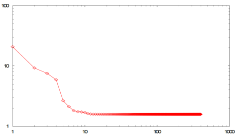
Figure 2: (Color online) Plot of the evolution of the sum of residuals for the $d=6$ case with four basis vs. the number of Monte Carlo steps. This typical evolution of the function to be optimized –the sum of residuals in our case– does not reach a minimum of zero. It approaches zero but the corresponding value is aways of $O(1)$. See text for details.

V Conclusions

We have translated the problem of the existence of $m=4-$bases in $\mathbb{C}^{6}$ into an optimization procedure. As expected, the concomitant numerical optimization has provided a satisfactory answer for known cases such as $m=3$ in $\mathbb{C}^{6}$. This new approach to the problem of to whether or not there exist a set of $m=4$ MU bases for $d=6$ has provided more evidence in favor that this is not case, although no theorem guarantees this argument.

In addition, we are left with the interesting question on the limitations that pose the use of sets of imperfect MU bases in quantum information tasks, an issue that is certainly of interest for in experiments one has to deal with imperfections. Also, our procedure is capable to explore more dimensions and bases in a straightforward manner, although taking into account that a computational limitation is reached, and therefore opens the door to similar studies in the future future .

References

- (1) J. Schwinger, Proc. Nat. Acad. Sci. U.S.A., 46, 560, (1960)
- (2) I. D. Ivanović, J. Phys. A, 14, 3241, (1981)
- (3) W. K. Wootters and B. D. Fields, Ann. Phys. (N.Y.), 191, 363 (1989)
- (4) C. Archer, J. Math. Phys. 46, 022106 (2005)
- (5) M. Planat, H. Rosu, and S. Perrine, Found. Phys. 36, 1662 (2006)
- (6) N. Cerf, M. Bourennane, A. Karlsson, and N. Gisin: Phys. Rev. Lett. 88, 127902 (2002)
- (7) S. Brierley: Quantum key distribution highly sensitive to eavesdropping, arXiv:0910.2578
- (8) Y. Aharonov and B. G. Englert, Z. Naturforsch A: Phys. Sci. 56, 16 (2001)
- (9) S. Brierley and S. Weigert, Phys. Rev. A 78, 042312 (2008)
- (10) S. Brierley and S. Weigert, Phys. Rev. A 79, 052316 (2009)
- (11) P. Raynal, X. L, and B.-G. Englert, Phys. Rev. A 83, 062303 (2011)
- (12) D. McNulty and S. Weigert, J. Phys. A: Math. Theor. 45, 102001 (2012)
- (13) W. Tadej and K. Zyczkowski, Open Sys. & Information Dyn. 13, 133 (2006)
- (14) S. Kirkpatrick, C. D. Gelatt Jr and M. P. Vecchi, Science 220 (4598), 671 (1983)
- (15) A. Haar, Ann. Math. 34, 147 (1933).
- (16) J. Conway, Course in Functional Analysis (Springer-Verlag, New York, 1990)
- (17) M. Chaichian and R. Hagedorn, Symmetries in quantum mechanics, (Inst. of Phys. Publ., Bristol)
- (18) M. L. Mehta, Random Matrices (Academic, New York, 1990)
- (19) A. Hurwitz, Nachr. Ges. Wiss. Gött. Math.-Phys. Kl. 71 (1887)
- (20) V. L. Girko, Theory of Random Determinants (Kluwer, Dordrecht, 1990)
- (21) T. Durt et al., Int. J. Quantum Information 8, 535 (2010)
- (22) D. Goyeneche, J. Phys. A: Math. Theor. 46, 105301 (2013)
- (23) P. Jaming et al, J. Phys. A: Math. Theor. 42, 245305 (2009)
- (24) J. Batle et al. Under preparation (2014)