Oblivious Query Processing

Abstract

Motivated by cloud security concerns, there is an increasing interest in database systems that can store and support queries over encrypted data. A common architecture for such systems is to use a trusted component such as a cryptographic co-processor for query processing that is used to securely decrypt data and perform computations in plaintext. The trusted component has limited memory, so most of the (input and intermediate) data is kept encrypted in an untrusted storage and moved to the trusted component on “demand.”

In this setting, even with strong encryption, the data access pattern from untrusted storage has the potential to reveal sensitive information; indeed, all existing systems that use a trusted component for query processing over encrypted data have this vulnerability. In this paper, we undertake the first formal study of secure query processing, where an adversary having full knowledge of the query (text) and observing the query execution learns nothing about the underlying database other than the result size of the query on the database. We introduce a simpler notion, oblivious query processing, and show formally that a query admits secure query processing iff it admits oblivious query processing. We present oblivious query processing algorithms for a rich class of database queries involving selections, joins, grouping and aggregation. For queries not handled by our algorithms, we provide some initial evidence that designing oblivious (and therefore secure) algorithms would be hard via reductions from two simple, well-studied problems that are generally believed to be hard. Our study of oblivious query processing also reveals interesting connections todatabase join theory.

1 Introduction

There is a trend towards moving database functionality to the cloud and many cloud providers have a database-as-a-service (DbaaS) offering [2, 21]. A DbaaS allows an application to store its database in the cloud and run queries over it. Moving a database to the cloud, while providing well-documented advantages [8], introduces data security concerns [28]. Any data stored on a cloud machine is potentially accessible to snooping administrators and to attackers who gain illegal access to cloud systems. There have been well-known instances of data security breaches arising from such adversaries [30].

A simple mechanism to address these security concerns is encryption. By keeping data stored in the cloud encrypted we can thwart the kinds of attacks mentioned above. However encryption makes computation and in particular query processing over data difficult. Standard encryption schemes are designed to “hide” data while we need to “see” data to perform computations over it. Addressing these challenges and designing database systems that support query processing over encrypted data is an active area of research [4, 6, 14, 27, 32] and industry effort [22, 23].

A common architecture [4, 6] for query processing over encrypted data involves using trusted hardware such as a cryptographic co-processor [16], designed to be inaccessible to an adversary. The trusted hardware has access to the encryption key, some computational capabilities, and limited storage. During query processing, encrypted data is moved to the trusted hardware, decrypted, and computed on. The trusted hardware has limited storage so it is infeasible to store within it the entire input database or intermediate results generated during query processing; these are typically stored encrypted in an untrusted storage and moved to the trusted hardware only when necessary. Other approaches to query processing over encrypted data rely on (partial) homomorphic encryption [14, 27, 32] or using the client as the trusted module [14, 32]. These approaches have limitations in terms of the class of queries they can handle or data shipping costs they incur (see Section 7), and they are not the main focus of this paper.

The systems that use trusted hardware currently provide an operational security guarantee that any data outside of trusted hardware is encrypted [4, 6]. However, this operational guarantee does not translate to end-to-end data security since, even with strong encryption, the data movement patterns to and from trusted hardware can potentially reveal information about the underlying data. We call such information leakage dynamic information leakage and we illustrate it using a simple join example.

Example 1

Consider a database with tables Patient (PatId,Name,City) and Visit(PatId,Date,Doctor) storing patient details and their doctor visits. These tables are encrypted by encrypting each record using a standard encryption scheme and stored in untrusted memory. Using suitably strong encryption, we can ensure that the adversary does not learn anything from the encrypted tables other than their sizes. (Such an encryption scheme is non-deterministic so two encryptions of the same record would look seemingly unrelated.)

Consider a query that joins these two tables on PatId column using a nested loop join algorithm. The algorithm moves each patient record to the trusted hardware where it is decrypted. For each patient record, all records of Visit table are moved one after the other to the trusted hardware and decrypted. Whenever the current patient record $p$ and visit record $v$ have the same PatId value, the join record $\langle p,v\rangle$ is encrypted and produced as output. An adversary observing the sequence of records being moved in and out of trusted hardware learns the join-graph. For example, if $5$ output records are produced in the time interval between the first and second Patient record moving to the trusted hardware, the adversary learns that some patient had $5$ doctor visits.

The above discussion raises the natural questionwhether we can design query processing algorithms that avoid such dynamic information leakage and provide end-to-end data security. The focus of this paper is to seek an answer to this question; in particular, as a contribution of this paper, we formalize a strong notion of (end-to-end) secure query processing, develop efficient and secure query processing algorithms for a large class of queries, and discuss why queries outside of this class are unlikely to have efficient secure algorithms.

There exists an extensive body of work ObliviousRAM (ORAM) Simulation [10, 12, 29, 33], a general technique that makes memory accesses of an arbitrary program appear random by continuously shuffling memory and adding spurious accesses. In Example 1, with ORAM simulation the data accesses would appear random to an adversary and we can show that the adversary learns no information other than the total number of data accesses.

Given general ORAM simulation, why design specialized secure query processing algorithms? We defer a full discussion of this issue to Section 1.2, but for a brief motivation consider sorting an encrypted array of size $n$. Just as in Example 1, the data access patterns of a standard sorting algorithm such as quicksort reveals information about the underlying data. An ORAM simulation of quicksort would hide the access patterns; indeed, the adversary does not even learn that a sort operation is being performed. However, with current state-of-the-art ORAM algorithms, it would incur an overhead of $\Theta(\log^{2}n)$ per access of the original algorithm making the overall complexity of sorting $\Theta(n\log^{3}n)$. Instead, we could exploit the semantics of sorting and design a secure sorting algorithm that has the (optimal) time complexity of $\Theta(n\log n)$ [11]. Here the adversary does learn that the operation being performed is sorting (but does not learn anything about the input being sorted) but we get significant performance benefits. As we show in the rest of the paper, designing specialized secure query processing algorithms helps us gain similar performance advantages over generic ORAM simulations.

The exploration in this paper is part of the Cipherbase project [7], a larger effort to design and prototype a comprehensive database system, relying on specialized hardware for storing and processing encrypted data in the cloud.

1.1 Overview of Contributions

Secure Query Processing: Informally, we define a query processing algorithm for a query $Q$ to be secure if an adversary having full knowledge of the text of $Q$ and observing the execution of $Q$ does not learn anything about the underlying database $D$ other than the result size of $Q$ over $D$. The query execution happens within a trusted module (TM) not accessible to the adversary. The input database and possibly intermediate results generated during query execution are stored (encrypted) in an untrusted memory (UM). The adversary has access to the untrusted memory and in particular can observe the sequence of memory locations accessed and data values read and written during query execution. Throughout, we assume a passive adversary, who does not actively interfere with query processing.

When defining security, we grant the adversary knowledge of query $Q$ which ensures that data security does not depend on the query being kept secret. Databases are typically accessed through applications and it is often easy to guess the query from a knowledge of the application. Our formal definition of secure query processing (Section 2.2) generalizes the informal definition above and incorporates query security in addition to data security. Our formal definition relies on machinery from standard cryptography such as indistinguishability experiments, but there are some subtleties specific to database systems and applications that we capture; Appendix A discusses these issues in greater detail.

We note that simply communicating the (encrypted) query result over an untrusted network reveals the result size, so a stronger notion of security seems impractical in a cloud setting. Also, our definition of secure query processing implies that an adversary with an access to the cloud server gets no advantage over an adversary who can observe only the communications between the client and the database server, assuming both of them have knowledge of the query.

Oblivious Query Processing Algorithms: Central to the idea of secure query processing is the notion of oblivious query processing. Informally, a query processing algorithm is oblivious if its (untrusted) memory access pattern is independent of the database contents once we fix the query and its input and output sizes. We can easily argue that any secure algorithm is oblivious: otherwise, the algorithm has different memory access patterns for different database instances, so the adversary learns something about the database instance by observing the memory access pattern of the algorithm. Interestingly, obliviousness is also a sufficient condition in the sense that any oblivious algorithm can be made secure using standard cryptography (Theorem 3). The idea of reducing security to memory access obliviousness was originally proposed in [10] for general programs in the context of software protection. Note that obliviousness is defined with respect to memory accesses to the untrusted store; any memory accesses internal to TM are invisible to the adversary and do not affect security.

Our challenge therefore is to design oblivious algorithms for database queries. We seek oblivious algorithms that have small TM memory footprint since all practical realizations of the trusted module such as cryptographic co-processors have limited storage (few MBs) [16]. Without this restriction a simple oblivious algorithm is to read the entire database into TM and perform query processing completely within TM.

To illustrate challenges in designing oblivious query processing algorithms consider the simple join query $R(A,\ldots)$ $\bowtie S(A,\ldots)$ which seeks all pairs of tuples from $R$ and $S$ that agree on attribute $A$. Figure 1 shows two instances for this join, represented as a binary “join-graph”. Each $R$ and $S$ tuple is shown as a vertex and its attribute $A$ value is shown adjacent to it (lower case letters $a,b,\ldots$). An edge exists between an $R$ tuple and an $S$ tuple having the same value in attribute $A$, and each edge represents a join output. We note that both instances have the same input output characteristics, $|R|=|S|=|R\bowtie S|=16$, so an oblivious algorithm is required to have the same memory access pattern for both instances. However, the internal structure of the join graph is greatly different. All “natural” join algorithms that use sorting or hashing to bring together joinable tuples are sensitive to the join graph structure and therefore not oblivious.

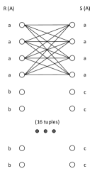
(a) Instance 1

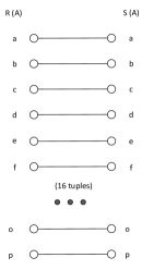
(b) Instance 2

Figure 1: Two join instances with same input/output sizes

Traditional database query processing is non-oblivious for two reasons: First, traditional query processing proceeds by identifying a query plan, which is a tree of operators with input tables at the leaves. The operators are (conceptually) evaluated in a bottom-up fashion and the output of each operator forms an input of its parent. In some cases, this bottom-up evaluation can be pipelined. In others, the output of an operator needs to be generated fully before the parent can consume it, and such intermediate output needs to be temporarily stored in untrusted memory. This renders the overall query processing non-oblivious since the size of the intermediate output can vary depending on the database instance, even if we fix input and output sizes. Second, standard implementations of database operators such as filters, joins, and grouping are not oblivious, so even if the query plan consisted of a single operator, the resulting query processing algorithm would not be oblivious. In summary, traditional query processing is non-oblivious at both inter- and intra-operator levels, and we need to fundamentally rethink query processing to make it oblivious.

Our first main algorithmic contribution is that a surprisingly rich class of database queries admit efficient oblivious algorithms (Sections 3, 4 and 5).

Theorem 1

(Informal) There exists an oblivious (secure) query processing algorithm that requires $O(\log n)$ storage in TM for any database query involving joins, grouping aggregation (as the outermost operation), and filters, if (1) the non-foreign key join graph is acyclic and (2) all grouping attributes are connected through foreign key joins, where $n$ denotes the sum of query input and output sizes. Further, assuming no auxiliary structures, the running time of the algorithm is within $O(\log n)$ (multiplicative factor) of the running time of the best insecure algorithm.

Theorem 1 suggests an interesting connection between secure query processing and database join theory since acyclic joins are a class of join queries known to be tractable [24]. We note that the class of queries is fairly broad and representative of real-world analytical queries. For example, most queries in the well-known TPC-H benchmark [31] belong to this class, i.e., admit efficient secure algorithms.

Assuming no auxiliary structures such as indexes, our algorithms are efficient and within $O(\log n)$ of the running time of the best insecure algorithm. While the no-index condition makes our results less relevant for transactional workloads, where indexes play an important role, they are quite relevant for analytical workloads where indexes play a less critical role. In fact, query processing in emerging database architectures such as column stores [1] has limited or no dependence on indexes.

Further, with minor modifications to our algorithms using the oblivious external memory sort algorithm of [13], we get oblivious and secure algorithms with excellent external (untrusted) memory characteristics.

Theorem 2

(Informal) For the class of queries in Theorem 1 there exists an oblivious (secure) algorithm with I/O complexity within multiplicative factor$\log_{M/B}(n/B)$ of that of the optimal insecure algorithm, where $B$ is the block size and $M$ is the TM memory.

In particular, if we have $\Omega(\sqrt{n})$ memory in TM our external memory algorithms perform a constant number of scans to evaluate the queries they handle.

Interestingly, for the special case of joins, secure algorithms have been studied in the context of privacy preserving data integration [19]. The algorithm proposed in [19] proceeds by computing a cross product of the input relations followed by a (secure) filter. Our algorithms are significantly more efficient and handle grouping and aggregation.

Negative Results: We have reason to believe that queries outside of the class specified in Theorem 1 do not admit secure efficient algorithms. We show that the existence of secure algorithms would imply more efficient algorithms for variants of classic hard problems such as 3SUM (Section 6). These hardness arguments suggest that we must accept a weaker notion of security if we wish to support a larger class of queries.

1.2 Oblivious RAM Simulations

ORAM simulations first proposed by Goldreich and Ostrovsky [10] is a general technique for making memory accesses oblivious that works for arbitrary programs. Specifically, ORAM simulation is the online transformation of an arbitrary program $P$ to an equivalent program $P^{\prime}$ whose memory accesses appear random (more precisely, drawn from some distribution that depends only on the number of memory accesses of $P$). By running $P^{\prime}$ within a secure CPU (TM) and using suitable encryption, an adversary observing the sequence of memory accesses to an untrusted memory learns nothing about $P$ and its data other than its number of memory accesses. Current ORAM simulation techniques work by adding a virtualization layer that continuously shuffles (untrusted) memory contents and adds spurious memory accesses, so that the resulting access pattern looks random.

A natural idea for oblivious query processing, implemented in a recent system [20], would be to run a standard query processing algorithm under ORAM simulation. However, the resulting query processing is not secure for our definition of security since it reveals more than just the output size. ORAM simulation, since it is designed for general programs, does not hide the total number of memory accesses; in the context of standard query processing, this reveals the size of intermediate results in a query plan. Understanding the utility of this weaker notion of security in the context of a database system is an interesting direction of future work.

For database queries that admit polynomial time algorithms (which includes queries covered by Theorem 1) we can design oblivious algorithms based on ORAM simulation: the number of memory accesses of such an algorithm is bounded by some polynomial $p(n,m)$, where $n$ is the input size, and $m$, the output size. We modify the algorithm with dummy memory accesses so that the number of memory accesses for any instance with input size $n$ and output size $m$ is exactly $p(n,m)$. An ORAM simulation of the modified algorithm is oblivious. We note that we need to precisely specify $p(n,m)$ upto constants (not asymptotically), otherwise the number of memory accesses would be slightly different for different $(n,m)$ intances making the overall algorithm non-oblivious. In practice, working out a precise upper-bound $p(n,m)$ for arbitrarily complex queries is a non-trivial undertaking.

Our algorithms which are designed to exploit the structure and semantics of queries have significant performance benefits over the ORAM-based technique sketched above given the current state-of-the-art in ORAM simulation. For simplicity, assume for this discussion that the query output size $m=O(n)$. For small TM memory ($\mathrm{polylog}(n)$), the current best ORAM simulation techniques [29, 18] incur an overhead of $\Theta(\log^{2}n)$ memory accesses per memory access of the original algorithm. This implies that the time complexity of any ORAM-based query processing algorithm is lower-bounded by $\Omega(n\log^{2}n)$. In contrast, our algorithms have a time complexity of $O(n\log n)$ and use $O(\log n)$ TM memory.

Also, by construction ORAM simulation randomly sprays memory accesses and destroys locality of reference, reducing effectiveness of caching and prefetching in a memory hierarchy. In a disk setting, a majority of memory accesses result in a random disk seek and we can show that any ORAM-based query processing algorithm incurs $\Omega(\frac{n}{B\log M}\log^{2}\frac{n}{B})$ disk seeks, where $M$ denotes the size of TM memory. In contrast, all of our algorithms are scan-based except for the oblivious sorting, which incurs $O(\log_{M/B}(n/B))\cdot o(n/B)$ seeks.

2 Problem formulation

2.1 Database Preliminaries

A relation schema, $R(\bar{A})$, consists of a relation symbol $R$ and associated attributes $\bar{A}=(A_{1},\ldots,A_{k})$; we use $\mathit{Attr}(R)$ to denote the set of attributes $\{A_{1},\ldots,A_{k}\}$ of $R$. An attribute $A_{i}$ has an associated set of values called its domain, denoted $\mathcal{D}(A_{i})$. We use $\mathcal{D}(R)$ to denote $\mathcal{D}(\bar{A})=\mathcal{D}(A_{1})\times\ldots\times\mathcal{D}(A_{k})$. A database schema is a set of relation schemas $R_{1},\ldots,R_{m}$. A (relation) instance corresponding to schema $R(A_{1},\ldots,A_{k})$ is a bag (multiset) of tuples of the form $\langle a_{1},\ldots,a_{k}\rangle$ where each $a_{i}\in\mathcal{D}(A_{i})$. A database instance is a set of relation instances. In the following we abuse notation and use the term relation (resp. database) to denote both relation schema and instance (resp. database schema and instance). We sometimes refer to relations as tables and attributes as columns.

Given a tuple $t\in R$ and an attribute $A\in\mathit{Attr}(R)$, $t[A]$ denotes the value of the tuple on attribute $A$; as a generalization of this notation, if $\mathcal{A}\subseteq\mathit{Attr}(R)$ is a set of attributes, $t[\mathcal{A}]$ denotes the tuple $t$ restricted to attributes in $\mathcal{A}$.

We consider two classes of database queries. A select-project-join (SPJ) query is of the form $\pi_{\mathcal{A}}(\sigma_{P}(R_{1}\bowtie\cdots\bowtie R_{q}))$, where the projection $\pi$ is duplicate preserving (we use multiset semantics for all queries) and $\bowtie$ refers to the natural join. For $R_{1}\bowtie R_{2}$, each tuple $t_{1}\in R_{1}$ joins with each tuple $t_{2}\in R_{2}$ such that $t_{1}[\mathit{Attr}(R_{1})\cap\mathit{Attr}(R_{2})]=t_{2}[\mathit{Attr}(R_{1})\cap\mathit{Attr}(R_{2})]$ to produce an output tuple $t$ over attributes $\mathit{Attr}(R_{1})\cup\mathit{Attr}(R_{2})$ that agrees with $t_{1}$ on attributes $\mathit{Attr}(R_{1})$ and with $t_{2}$ on attributes $\mathit{Attr}(R_{2})$. The second class of queries involves grouping and aggregation and is of the form $\mathbbm{G}_{\mathcal{G}}^{F(A)}(\sigma_{P}(R_{1}\bowtie\cdots\bowtie R_{q}))$ and we call such queries GSPJ queries. Given relation $R$, $\mathcal{G}\subseteq\mathit{Attr}(R)$, $A\in\mathit{Attr}(R)$, $\mathbbm{G}_{\mathcal{G}}^{F(A)}(R)$, represents grouping by attributes in $\mathcal{G}$ and computing aggregation function $F$ over attribute $A$.

2.2 Secure Query Processing

A relation encryption scheme is used to encrypt relations. It is a triple of polynomial algorithms $(\textsf{Enc},\textsf{Dec},\textsf{Gen})$ where Gen takes a security parameter $k$ and returns a key $K$; Enc takes a key $K$, a plaintext relation instance $R$ and returns a ciphertext relation $\mathcal{C}_{R}$; Dec takes a ciphertext relation $\mathcal{C}_{R}$ and key $K$ and returns plaintext relation $R$ if $K$ was the key under which $\mathcal{C}_{R}$ was produced. A relation encryption scheme is also a database encryption scheme: to encrypt a database instance we simply encrypt each relation in the database.

Informally, a relation encryption scheme is IND-CPA secure if a polynomial time adversary with access to encryption oracle cannot distinguish between the encryption of two instances $R^{(1)}$ and $R^{(2)}$ of relation schema $R$ such that $|R^{(1)}|=|R^{(2)}|$ ($|R^{(1)}|$ denotes the number of tuples in $R^{(1)}$). Assuming all tuples of a given schema have the same representational length (or can be made so using padding), we can construct IND-CPA secure relation encryption by encrypting each tuple using a standard encryption scheme such as AES in CBC mode (which is believed to be IND-CPA secure for message encryption). The detail that encryption is at a tuple-granularity is relevant for our algorithms which assume that we can read and decrypt one tuple at a time.

Our formal definition of secure query processing captures: (1) Database security: An adversary with knowledge of a query does not learn anything other than the result size of the query by observing query execution; (2) Query security: An adversary without knowledge of the query does not learn the constants in the query from query execution. Appendix A contains a discussion of query security.

A query template $\mathcal{Q}$ is a set of queries that differ only in constants. An example template is the set $\{\sigma_{A=1}(R),$ $\sigma_{A=2}(R),\cdots\}$ which we denote $\sigma_{A=*}(R)$.

A query processing algorithm $\mathbb{A}_{\mathcal{Q}}$ for a query template $\mathcal{Q}$ takes as input an encrypted database instance $\textsf{Enc}_{K}(D)$, a query $Q\in\mathcal{Q}$ and produces as output$\textsf{Enc}_{K}(Q(D))$; Algorithm $\mathbb{A}_{\mathcal{Q}}$ has access to encryption key $K$ and the encryption scheme is IND-CPA secure. Our goal is to make algorithm $\mathbb{A}_{\mathcal{Q}}$ secure against a passive adversary who observes its execution. Algorithm $\mathbb{A}_{\mathcal{Q}}$ runs within the trusted module TM. The TM also has a small amount of internal storage invisible to the adversary. Algorithm $\mathbb{A}_{\mathcal{Q}}$ has access to a large amount of untrusted storage which is sufficient to store $\textsf{Enc}_{K}(D)$ and any intermediate state required by $\mathbb{A}_{\mathcal{Q}}$. The trace of an execution of algorithm $\mathbb{A}_{\mathcal{Q}}$ is the sequence of untrusted memory accesses $\mathit{read}(i)$ and $\mathit{write}(i,\mathit{value})$, where $i$ denotes the memory location.

We define security of algorithm $\mathbb{A}_{\mathcal{Q}}$ using the following indistinguishability experiment:

1. Pick $K\leftarrow\textsf{Gen}(1^{k})$

2. The adversary $\mathcal{A}$ picks two queries $Q_{1}\in\mathcal{Q}$, $Q_{2}\in\mathcal{Q}$ with the same template and two database instances $D^{(1)}=\{R_{1}^{(1)},\ldots,$ $R_{n}^{(1)}\}$ and $D^{(2)}=$$\{R_{1}^{(2)},\ldots,R_{n}^{(2)}\}$ having the same schema such that (1) $|R_{i}^{(1)}|=|R_{i}^{(2)}|$ for all $i\in[1,n]$; and (2)$|Q_{1}(D^{(1)})|=|Q_{2}(D^{(2)})|$.

3. Pick a random bit $b\leftarrow\{0,1\}$ and let $\tau_{b}$ denote the trace of $\mathbb{A}_{\mathcal{Q}}(\textsf{Enc}_{K}(D^{(b)}),$ $Q_{b})$.

4. The adversary $\mathcal{A}$ outputs prediction $b^{\prime}$ given $\tau_{b}$, $\textsf{Enc}_{K}(D^{(b)})$, and $\textsf{Enc}_{K}(Q_{b}(D^{(b)}))$.

We say adversary $\mathcal{A}$ succeeds if $b^{\prime}=b$. Algorithm $\mathbb{A}_{\mathcal{Q}}$ is secure if for any polynomial time adversary $\mathcal{A}$, the probability of success is at most $1/2+\mathit{negl}(k)$ for some negligible function $\mathit{negl}$. We note that our definition of security captures both database security, since an adversary can pick $Q_{1}=Q_{2}$, and query security, since an adversary can pick $D^{(1)}=D^{(2)}$.

2.3 Oblivious Query Processing

As discussed in Section 1, oblivious query processing is a simpler notion that is equivalent to secure query processing. Fix an algorithm $\mathbb{A}_{\mathcal{Q}}$. For an input $I=\textsf{Enc}_{K}(D)$ and query $Q\in\mathcal{Q}$, the memory access sequence $\mathcal{M}_{\mathbb{A}_{\mathcal{Q}}}(I,Q)$ is the sequence of UM memory reads $r(i)$ and writes $w(i)$, where $i$ denotes the memory location; the value being read/written is not part of$\mathcal{M}_{\mathbb{A}_{\mathcal{Q}}}(I,Q)$. In general, $\mathbb{A}_{\mathcal{Q}}$ is randomized and$\mathcal{M}_{\mathbb{A}_{\mathcal{Q}}}(I,Q)$ is a random variable defined over all possible memory access sequences. Algorithm $\mathbb{A}_{\mathcal{Q}}$ is oblivious if the distribution of its memory access sequences is independent of database contents once we fix the query output and database size. Formally, Algorithm $\mathbb{A}_{\mathcal{Q}}$ is oblivious if for any memory access sequence $M$, any two queries $Q_{1},Q_{2}\in\mathcal{Q}$, any two database encryptions $I_{1}=\textsf{Enc}_{K_{1}}(D^{(1)})$, $I_{2}=\textsf{Enc}_{K_{2}}(D^{(2)})$:

$$\mathrm{Pr}[\mathcal{M}_{\mathbb{A}_{\mathcal{Q}}}(I_{1},Q_{1})=M]=\mathrm{Pr}[\mathcal{M}_{\mathbb{A}_{\mathcal{Q}}}(I_{2},Q_{2})=M]$$

where $D^{(1)}=\{R_{1}^{(1)},\ldots,R_{n}^{(1)}\}$ and $D^{(2)}=\{R_{1}^{(2)},\ldots,$ $R_{n}^{(2)}\}$ have the same schema and: (1) $|R_{i}^{(1)}|=|R_{i}^{(2)}|$ for all $i\in[1,n]$; and (2) $|Q_{1}(D^{(1)})|=|Q_{2}(D^{(2)})|$.

Our definition of obliviousness is more stringent than the one used in ORAM simulation. In ORAM simulation, the memory access distribution can depend on the total number of memory accesses, while our definition precludes dependence on the total number of memory accesses once the query input and output sizes are fixed. The following theorem establishes the connection between oblivious and secure query processing.

Theorem 3

Assuming one-way functions exist, the existence of an oblivious algorithm for a query template $\mathcal{Q}$ implies the existence of a secure algorithm for $\mathcal{Q}$ with the same asymptotic performance characteristics (TM memory required, running time).

The idea of using obliviousness to derive security from access pattern leakage was originally proposed in [10] and the proof of Theorem 3 is similar to the proof of analogous Theorem 3.1.1 in [10]. Informally, we get secure query processing by ensuring both data security of values stored in untrusted memory and access pattern obliviousness. Data security can be achieved by using encryption, and secure encryption schemes exist assuming the existence of one-way functions. It follows that the existence of oblivious query processing algorithms implies the existence of secure algorithms. Based on Theorem 3, the rest of the paper focuses on oblivious query processing and does not directly deal with encryption and data security.

3 Intuition

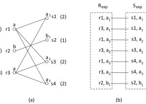
Figure 2: Illustration of Oblivious Binary Join

This section presents a high level intuition behind our algorithms. Consider the binary join $R(A,\ldots)\bowtie S(A,\ldots)$ and the join graph instance shown in Figure 2(a). Lower case letters $a$, $b$, represent values of the joining column $A$; ignore the subscripts on $a$ and $b$ for now. We add identifiers $r_{1}$-$r_{3}$ and $s_{1}$-$s_{4}$ to tuples so that we can refer to them in text.

Our oblivious binary join algorithm works in twostages: In the first stage, we compute the contribution of each tuple to the final output. This is simply the degree of the tuple in the join graph; this value is shown within parenthesis in Figure 2(a). For example, the degree of $r_{1}$ is $3$, and degree of $r_{2}$, $1$. In the second stage, we expand $R$ to $R_{exp}$ by duplicating each tuple as many times as its degree; $r_{1}$ occurs $3$ times in $R_{exp}$, $r_{2}$ once, and so on. We similarly, expand $S$ to $S_{exp}$. The expansions $R_{exp}$ and $S_{exp}$ are shown within boxed rectangles in Figure 2(b). The final join output is produced by “stitching” together $R_{exp}$ and $S_{exp}$ as illustrated in Figure 2(b). The expansions $R_{exp}$ and $S_{exp}$ are sequences whose ordering is picked carefully to ensure that stitching the $i$th tuple in $R_{exp}$ with the $i$th tuple in $S_{exp}$ indeed produces the correct join output.

A central component of the above algorithm are oblivious implementations of two simple primitives that we call semi-join aggregation and expansion. Semi-join aggregation computes the degree of each tuple in a join and expansion expands a relation by duplicating each tuple a certain number of times such as its degree.

The same approach generalizes to multiway joins if the overall query is acyclic [24]. Informally, to compute $R\bowtie S\bowtie T$, we would compute the contribution of each tuple to the final join output and use these values to expand input relations to $R_{exp}$, $S_{exp}$, and $T_{exp}$, which are then stitched together to produce the final join output.

4 Primitives

This section introduces a few core primitives andpresents oblivious algorithms—algorithms that have the same UM memory access patterns once we fix input and output sizes—for these primitives. These primitives serve two purposes: First, as discussed in Section 3, they are building blocks for our oblivious query processing algorithms; Second, they introduce notation to help us concisely specify our algorithms, and reason about their obliviousness and performance.

There exist oblivious algorithms for all the primitives of this section having time complexity $O(n\log n)$ and requiring $O(\log n)$ TM memory, where $n$ denotes the sum of input and output sizes. Some of these algorithms rely on an oblivious sort; an optimal $O(n\log n)$ oblivious sort algorithm that uses $O(1)$ TM memory is presented in [11]. Due to space constraints we defer presenting oblivious algorithms for the simpler primitives to the full version of the paper [5].

$A$ $r_{1}$ $1$ $r_{2}$ $2$ $r_{3}$ $1$	$A$ $B$ $s_{1}$ $1$ $1$ $s_{2}$ $2$ $1$ $s_{3}$ $2$ $1$	$A$ $B$ $C$ $D$ $E$ $1$ $2$ $1$ $2$ $1$ $2$ $4$ $1$ $6$ $2$ $1$ $2$ $2$ $8$ $1$
$R$	$S$	$\tilde{R}$

Figure 3: Illustration of primitives: $\tilde{R}\leftarrow R.(B\leftarrow 2A).(C\leftarrow\mathrm{ID}_{A}).(D\leftarrow\mathrm{RSum}(B)).(E\stackrel{{\scriptstyle\ltimes}}{{\leftarrow}}\mathit{Sum}(S.B))$. $r_{1}$-$r_{3}$ and $s_{1}$-$s_{3}$ are names we use to refer to the tuples.

Relation Augmentation: This primitive adds a derived column to a relation. In the simplest form the derived column is obtained by applying a function to existing columns; many primitives we introduce subsequently are more complex instantiations of relation augmentation. We use the notation $R.(A\leftarrow\mathit{Func})$ to represent relation augmentation which adds a new derived column $A$ using some function $\mathit{Func}$ and produces an output relation with schema $\mathit{Attr}(R)\cup\{A\}$. For example, $R.(B\leftarrow 2A)$ adds a new column $B$ whose value is twice that of $A$ (see Figure 3). Our notation allows composition to be expressed more concisely; e.g., $R.(B\leftarrow 2A).(F\leftarrow A+B)$.

Grouping Identity: This relation augmentation primitive adds a new identity column within a group; identity column values are of the form $1,2,\ldots$. In particular, we use the notation $R.(A\leftarrow\mathrm{ID}_{\mathcal{G}}^{\mathcal{O}})$ where $\mathcal{G}\subseteq\mathit{Attr}(R)$ is a set of grouping columns and $\mathcal{O}\subseteq\mathit{Attr}(R)$ is a set of ordering columns. To get the output, we partition the tuples by the grouping columns $\mathcal{G}$, order the tuples within each partition by $\mathcal{O}$, and assign ids based on this ordering. (We break ties arbitrarily, so the output can be non-deterministic.) $\mathcal{G}$ and $\mathcal{O}$ can be empty and omitted. For example, $R.(Id\leftarrow\mathrm{ID})$ assigns an unique id to each record in $R$. In Figure 3, for $R.(C\leftarrow\mathrm{ID}_{A})$, we partition by $A$, so $r_{1}$ and $r_{3}$ go to the same partition; tuple $r_{1}$ gets a $C$ value of $1$, and $r_{3}$, a $C$ value of $2$.

Grouping Running Sum: This primitive is a generalization of grouping identity and adds a running sum column to a relation. It is represented$R.(A\leftarrow\mathrm{RSum}_{\mathcal{G}}^{\mathcal{O}}(B))$; it groups a relation by $\mathcal{G}$ and orders tuples in a group by $\mathcal{O}$ and stores the running sum of $B$ column values in a new column $A$. In particular, grouping identity $R.(\mathit{Id}\leftarrow\mathrm{ID}_{\mathcal{G}}^{\mathcal{O}})$ can be expressed as $R.(X\leftarrow 1).(\mathit{Id}\leftarrow\mathrm{RSum}_{\mathcal{G}}^{\mathcal{O}}(X))$. See Figure 3 for an example.

Generalized Union: A generalized union of $R$ and $S$, denoted $R\bar{\cup}S$, produces a relation with schema $\mathit{Attr}(R)\cup\mathit{Attr}(S)$ that contains tuples from both $R$ and $S$. Tuples of $R$ have a null value for attributes in $\mathit{Attr}(S)-\mathit{Attr}(R)$, and those of $S$, a null value for attributes in $\mathit{Attr}(R)-\mathit{Attr}(S)$.

Sequences: Sorting and Stitching: Although the inputs and outputs of our algorithms are relations represented as sequences, the ordering is often unimportant and we mostly do not emphasize the sequentiality. We use the notation $\langle R\rangle$ to represent some sequence corresponding to $R$. When a particular ordering is desired, we represent the ordering as $\langle R\rangle_{\mathcal{O}}$ where $\mathcal{O}\subseteq\mathit{Attr}(R)$ denote the ordering attributes.

One operation on sequences that cannot be represented over bags is “stitching” two sequences of the same length (see Figure 2(b) for an example): Given two sequences $\langle R\rangle$ and $\langle S\rangle$ of the same length $n$, the operation $\langle R\rangle\cdot\langle S\rangle$ produces a sequence of length $n$ with schema $\mathit{Attr}(R)\cup\mathit{Attr}(S)$ and the $i$th tuple of the sequence is obtained by concatenating the $i$th tuple of $\langle R\rangle$ and the $i$th tuple of $\langle S\rangle$; we ensure when invoking this operation that the $i$th tuples of both sequences agree on $\mathit{Attr}(R)\cap\mathit{Attr}(S)$ if the intersection is nonempty.

Filters: Consider the filter $\sigma_{P}(R)$. The simple algorithm that scans each tuple $t\in R$, checks if it satisfies $P$, and outputs it if does, is not oblivious. (E.g., simply reordering tuples in $R$ changes the memory write pattern.)

The oblivious sorting algorithm can be used to design a simple oblivious algorithm for selection (filter). To evaluate $\sigma_{P}(R)$, we sort $R$ such that tuples that satisfy predicate $P$ occur before tuples that do not. We scan the sorted table and output the tuples that satisfy $P$ and stop when we encounter the first tuple that does not satisfy $P$. The overall data access pattern depends only on input and output sizes and is therefore oblivious.

4.1 Semi-Join Aggregation

Semi-join aggregation, denoted $R.(A\stackrel{{\scriptstyle\ltimes}}{{\leftarrow}}\mathit{Sum}(S.B))$, is equivalent to the relational algebra expression$\mathbbm{G}_{\mathit{Attr}(R)}^{A\leftarrow\mathrm{SUM}(S.B)}(R\bowtie S)$. This operation adds a new derived column $A$; for each tuple $t_{R}\in R$, we obtain value of $A$ by identifying all $t_{S}\in S$ that join with $t_{R}$ (agree on all common attributes $\mathit{Attr}(R)\cap\mathit{Attr}(S)$) and summing over $t_{S}[B]$ values. As discussed in Section 3, we introduce this primitive to compute the degree of a tuple in a join graph. In particular, the degree of each $R$ tuple in $R\bowtie S$ is obtained by $\tilde{S}\leftarrow S.(X\leftarrow 1)$, $R.(\mathit{Degree}\stackrel{{\scriptstyle\ltimes}}{{\leftarrow}}\mathit{Sum}(\tilde{S}.X))$. In Figure 3, $r_{2}$ joins with two tuples $s_{2}$ and $s_{3}$, so $r_{2}[E]$ is $s_{2}[B]+s_{3}[B]=2$.

Algorithm 1 Semi-Join Aggregation: $R.(X\stackrel{{\scriptstyle\ltimes}}{{\leftarrow}}\mathit{Sum}(S.Y))$

1:procedure SemiJoinAgg($R,S,X,Y$)

2:    $\tilde{R}\leftarrow R.(\mathit{Src}\leftarrow 1).(Y\leftarrow 0)$

3:    $\tilde{S}\leftarrow S.(\mathit{Src}\leftarrow 0)$

4:    $U\leftarrow\tilde{R}\ \bar{\cup}\ \tilde{S}$

5:    $U\leftarrow U.(X\leftarrow\mathrm{RSum}_{\mathit{Attr}(R)\cap\mathit{Attr}(S)}^{\mathit{Src}}(Y))$

6:    Output $\pi_{\mathit{Attr}(R),X}(\sigma_{\mathit{Src}=1}(U))$

7:end procedure

Oblivious Algorithm: Algorithm 1 presents an oblivious algorithm for semi-join aggregation$R.(X\stackrel{{\scriptstyle\ltimes}}{{\leftarrow}}\mathit{Sum}(S.Y))$. (In all our algorithms, each step involves one of our primitives and is implemented using the oblivious algorithm for the primitive.) It adds a “lineage” column $\mathit{Src}$ in Steps 2 and 3; the value of $\mathit{Src}$ is set to $1$ for all $R$ tuples and $0$ for all $S$ tuples. A $Y$ column initialized to $0$ is added to all $R$ tuples. Step 4 computes a generalized union $U$ of $\tilde{R}$ and $\tilde{S}$. Adding the running sum within each $\mathit{Attr}(R)\cap\mathit{Attr}(S)$ group adds the required aggregation value into each $R$ tuple (Step 5); the running sum computation is ordered by $\mathit{Src}$ to ensure that all $S$ tuples within an $\mathit{Attr}(R)\cap\mathit{Attr}(S)$ group occur before the $R$ tuples. Finally, the oblivious filter $\sigma_{\mathit{Src}=1}$ in Step 6 extracts the $R$ tuples from $U$. Figure 4 shows the intermediate tables generated by Algorithm 1 for sample tables $R(Id,A)$ and $S(A,Y)$.

$\mathit{Id}$ $A$ $Y$ $\mathit{Src}$ 1 a 0 1 2 b 0 1	$A$ $Y$ $\mathit{Src}$ a 2 0 b 3 0 a 4 0	$\mathit{Id}$ $A$ $Y$ $\mathit{Src}$ $X$ - a 2 0 2 - a 4 0 6 1 a 0 1 6 - b 3 0 3 2 b 0 1 3
(a): $\tilde{R}$	(b): $\tilde{S}$	(c): $U$

Figure 4: Sample computation of $R.(X\stackrel{{\scriptstyle\ltimes}}{{\leftarrow}}\mathit{Sum}(S.Y))$

Theorem 4

Algorithm 1 obliviously computes semi-join aggregation $R.(X\stackrel{{\scriptstyle\ltimes}}{{\leftarrow}}\mathit{Sum}(S.Y))$ of two tables in $O((n_{R}+n_{S})\log(n_{R}+n_{S}))$ time and using $O(1)$ TM memory, where $n_{R}=|R|$ and $n_{S}=|S|$ denote the input table sizes.

Proof 4.5.

(Sketch) For each step of Algorithm 1 the input and output sizes are one of $n_{R}$, $n_{S}$, and $n_{R}+n_{S}$ and each step is locally oblivious in its input and output sizes. The overall algorithm is therefore oblivious. Further, the oblivious algorithms for each step require $O(1)$ TM memory.

4.2 Expansion

This primitive duplicates each tuple of a relation a number of times as specified in one of the columns. In particular, the output of $\mathrm{Exp}_{W}(R)$, $W\in\mathit{Attr}(R)$ and $\mathcal{D}(W)\subseteq\mathbb{N}$ is a relation instance with same schema, $\mathit{Attr}(R)$, that has $t[W]$ copies of each tuple $t\in R$. For example, given an instance of $R(A,W):\{\langle a,1\rangle,\langle b,2\rangle\}$, $\mathrm{Exp}_{W}(R)$ is given by $\{\langle a,1\rangle,\langle b,2\rangle,\langle b,2\rangle\}$. As discussed in Section 3, expansion plays a central role in our join algorithms.

4.2.1 Oblivious Algorithm

We now present an oblivious algorithm to compute $\mathrm{Exp}_{W}(R)$. For presentational simplicity, we slightly modify the representation of the input. The modified input to the expansion is a sequence of pairs $(\langle r_{1},w_{1}\rangle,$ $\ldots,\langle r_{n},w_{n}\rangle)$, where $r_{i}$s are values (tuples) drawn from some domain and $w_{i}\in\mathbb{N}$ are non-negative weights. The desired output is some sequence containing (in any order) $w_{i}$ copies of each $r_{i}$. We call such a sequence a weighted sequence.

The input size of expansion is $n$ and the output size is $m\stackrel{{\scriptstyle\mathrm{def}}}{{=}}\sum_{i=1}^{n}w_{i}$, so memory access pattern of an oblivious algorithm depends on only these two quantities. The naive algorithm that reads each $\langle r_{i},w_{i}\rangle$ into TM and writes out $w_{i}$ copies of $r_{i}$ is not oblivious, since the output pattern depends on individual weights $w_{i}$.

We first present an oblivious algorithm when the input sequence has a particular property we call prefix-heavy; we use this algorithm as a subroutine in the algorithm for the general case.

Definition 4.6.

A weighted sequence $(\langle r_{1},w_{1}\rangle,$ $\ldots,$$\langle r_{n},w_{n}\rangle)$ is prefix-heavy if for each $\ell\in[1,n]$,$\frac{1}{\ell}\sum_{i=1}^{\ell}w_{i}\geq\frac{1}{n}\sum_{i=1}^{n}w_{i}$.

The average weight of any prefix of a prefix-heavy sequence is greater-than-or-equal to the overall average weight. Any weighted sequence can be reordered to get a prefix-heavy sequence, e.g., by sorting by non-decreasing weight. The sequence $(\langle a,4\rangle,\langle b,1\rangle,$ $\langle c,2\rangle)$ is prefix-heavy, while $(\langle b,1\rangle,$ $\langle a,4\rangle,\langle c,2\rangle)$ is not.

Algorithm 2 Oblivious Expansion of prefix heavy sequences

1:procedure ExpandPrefixHeavy($I$)

2:Assume: $I=(\langle r_{1},w_{1}\rangle,\ldots,\langle r_{n},w_{n}\rangle)$

3:Require: $I$ is prefix heavy

4:    $w_{\mathit{avg}}\leftarrow(\sum_{i=1}^{n}w_{i})/n$

5:    $\mathcal{C}_{TM}\leftarrow\phi$ $\triangleright$ counters within TM

6:    for $i=1$ to $n$ do

7:         Read $\langle r_{i},w_{i}\rangle$ to TM.

8:         $w_{\mathit{curr}}\leftarrow\lfloor i\cdot w_{\mathit{avg}}\rfloor-\lfloor(i-1)\cdot w_{\mathit{avg}}\rfloor$

9:         if $w_{i}\leq w_{\mathit{curr}}$ then

10:             Append $w_{i}$ copies of $r_{i}$ to output

11:             $w_{\mathit{curr}}\leftarrow w_{\mathit{curr}}-w_{i}$

12:         else

13:             $\mathcal{C}_{TM}[r_{i}]\leftarrow w_{i}$

14:         end if

15:         while $w_{\mathit{curr}}>0$ do

16:             $r_{j}\leftarrow\mathrm{argmin}_{k}$ $r_{k}$ has a counter in $\mathcal{C}_{TM}$

17:             if $\mathcal{C}_{TM}[r_{j}]>w_{\mathit{curr}}$ then

18:                 Append $w_{\mathit{curr}}$ copies of $r_{j}$ to output

19:                 $\mathcal{C}_{TM}[r_{j}]\leftarrow\mathcal{C}_{TM}[r_{j}]-w_{\mathit{curr}}$

20:                 $w_{\mathit{curr}}\leftarrow 0$

21:             else

22:                 Append $\mathcal{C}_{TM}[r_{j}]$ copies of $r_{j}$ to output

23:                 $w_{\mathit{curr}}\leftarrow w_{\mathit{curr}}-\mathcal{C}_{TM}[r_{j}]$

24:                 // $\mathcal{C}_{TM}[r_{j}]\leftarrow 0$

25:                 Remove $r_{j}$ from $\mathcal{C}_{TM}$

26:             end if

27:         end while

28:    endfor

29:end procedure

Algorithm 2 presents an oblivious algorithm for expanding prefix heavy weighted sequences. To expand the sequence $I=(\langle r_{1},w_{1}\rangle,$ $\ldots,\langle r_{n},w_{n}\rangle)$, the algorithm proceeds in $n$ (input-output) steps. Let $w_{\mathit{avg}}=(\sum_{i=1}^{n}w_{i})/n$ denote the average weight of the sequence. In each step, it reads one weighted record (Step 7) and produces $w_{\mathit{avg}}$ (unweighted) records in the output; the actual number $w_{\mathit{curr}}$ is either $\lfloor w_{\mathit{avg}}\rfloor$ or $\lceil w_{\mathit{avg}}\rceil$, when $w_{\mathit{avg}}$ is fractional (Step 8).

Call a record $\langle r_{i},w_{i}\rangle$ light if $w_{i}\leq w_{\mathit{avg}}$ and heavy, otherwise. If the current record $\langle r_{i},w_{i}\rangle$ is light, $w_{i}$ copies of $r_{i}$ are produced in the output; if it is heavy, a counter $\mathcal{C}[r_{i}]$ is initialized with count $w_{i}$ denoting the number of copies of $r_{i}$ available for (future) outputs. Previously seen heavy records are used to make up the “balance” and ensure $w_{\mathit{avg}}$ records are produced in each step. The counters $\mathcal{C}$ are internal to TM and are not part of the data access pattern. Figure 5 shows the steps of Algorithm 2 for the sequence $(\langle a,4\rangle,\langle b,1\rangle,\langle c,2\rangle)$.

Step	Input	Output	Counters
1	$\langle a,4\rangle$	$a,a$	$\mathcal{C}[a]=2$
2	$\langle b,1\rangle$	$b,a,a$	$\mathcal{C}=\phi$
3	$\langle c,2\rangle$	$c,c$	$\mathcal{C}=\phi$

Figure 5: Algorithm 2 over sequence $(\langle a,4\rangle,\langle b,1\rangle,\langle c,2\rangle)$

Algorithm 2 is oblivious since its input-output pattern is fixed once the input size $n$ and output size $m=\sum_{i=1}^{n}w_{i}$ is fixed. Note that $w_{\mathit{avg}}=m/n$ is fixed once input and output sizes are fixed.

In the worst case, the number of counters maintained by Algorithm 2 can be $\Omega(n)$.

Example 4.7.

Consider the sequence $w_{1}=\cdots=w_{n/4}=4$ and $w_{n/2+1}=\cdots=w_{n}=0$. After reading $n/4$ records, we can show that Algorithm 2 requires $\approx 3n/16$ counters.

However, any weighted sequence can be re-ordered so that it is prefix heavy and the number of counters used by Algorithm 2 is $O(1)$ as stated in Lemma 4.9 and illustrated in the following example.

Example 4.8.

We can reorder the weight sequence in Example 4.7 as $\langle 4,0,0,0,4,0,0,0,\ldots,\rangle$ interleaving $3$ light records inbetween two heavy records. We can show that Algorithm 2 requires just one counter for this sequence.

More generally, the basic idea is to interleave sufficient number of light records between two heavy records so that average weight of any prefix is barely above the overall average, which translates to fewer number of counters. In Example 4.8, we can suppress just one heavy record to make the average weight of any prefix $\leq w_{\mathit{avg}}$. We call such sequences barely prefix heavy.

Lemma 4.9.

Any weighted sequence $I$ can be re-ordered as a prefix heavy sequence $I^{\prime}$ such that Algorithm 2 requires $O(1)$ counters to process $I^{\prime}$.

Lemma 4.9 suggests that we can design a general algorithm for expansion by first reordering the input sequence to be barely prefix heavy and using Algorithm 2. The main difficulty lies in obliviously reordering the sequence to make it barely prefix heavy. We do not know how to do this directly; instead, we transform the input sequence to a modified sequence by rounding weights (upwards) to be a power of $2$. We can concisely represent the full rounded weight distribution using logarithmic space. We store this rounded distribution within TM and use it to generate a barely prefix heavy sequence. Details of the algorithm to reorder a sequence to make it barely prefix heavy is presented in the full-version of the paper [5].

Algorithm 3 Oblivious Expansion $\mathrm{Exp}_{W}(R)$

1:procedure Expand($R,W$)

2:    $m\leftarrow\mathbbm{G}^{\mathrm{SUM}(W)}$ $\triangleright$ output size

3:    $\tilde{R}\leftarrow R.(\tilde{W}\leftarrow 2^{\lceil\log_{2}W\rceil})$ $\triangleright$ weight rounding

4:    $\tilde{m}\leftarrow\mathbbm{G}^{\mathrm{SUM}(\tilde{W})}$ $\triangleright$ assert: $\tilde{m}<2m$

5:    $\tilde{R}\leftarrow\tilde{R}\ \bar{\cup}\ \{\langle\mathit{dummy}\rangle\}.(W\leftarrow 0).(\tilde{W}\leftarrow 2m-\tilde{m})$

6:    $\mathcal{D}_{TM}\leftarrow\mathbbm{G}_{\tilde{W}}^{\mathrm{COUNT(*)}}(\tilde{R})$ $\triangleright$ rounded weight distr

7:    $\tilde{R}\leftarrow\tilde{R}.(\mathit{Id}\leftarrow\mathrm{ID})$ $\triangleright$ Attach ids

8:    $\langle\tilde{R}_{bph}\rangle\leftarrow$ReorderBarelyPrefixHeavy$(\tilde{R},\tilde{D}_{TM})$

9:    $\tilde{R}_{\mathit{exp}}\leftarrow$ExpandPrefixHeavy$(\langle\tilde{R}_{bph}\rangle)$

10:    $\tilde{R}_{\mathit{exp}}\leftarrow\tilde{R}_{\mathit{exp}}.(\mathit{Rank}\leftarrow\mathrm{ID}_{\mathit{Id}})$

11:    Output $\pi_{\mathit{Attr}(R)}(\sigma_{\mathit{Rank}<=W}(\tilde{R}_{\mathit{exp}}))$

12:end procedure

Algorithm 3 presents our oblivious expansion algorithm. Step 3 performs weight rounding. Directly expanding with these rounded weights produces a sequence of length $\tilde{m}$; the resulting algorithm would not be oblivious since $\tilde{m}$ does not depend on $n$ and $m$ (output size) alone. We therefore add (Step 5) a dummy tuple with rounded weight $2m-\tilde{m}$ (and actual weight $0$). Expanding this table produces $2m$ tuples. Step 6 computes the distribution of rounded weights. We note that this step consumes $\tilde{R}$ and produces no output since $\mathcal{D}_{TM}$ remains within TM. Step 8 reorders the table (sequence) to make it barely prefix heavy which is expanded using Algorithm 2 in Step 9. Steps 10 and 11 filter out dummy tuples produced due to rounding using an oblivious selection algorithm.

Theorem 4.10.

Algorithm 3 obliviously expands an input table in time $O((n+m)\log(n+m))$ using $O(\log(n+m))$ TM memory, where $n$ and $m$ denote the input and output sizes, respectively.

Proof 4.11.

(Sketch) The input size of each step is one of $n$, $n+1$ or $m$. The output size of each step is one of $1$, $n$, $n+1$, or $m$. Each step is locally oblivious, so all data access patterns are fixed once we fix $n$ and $m$.

5 Query Processing Algorithms

We now present oblivious query processing algorithms for SPJ and GSPJ queries. Recall from Section 2.1 that these are of the form $\pi_{\mathcal{A}}(\sigma_{P}(R_{1}\bowtie\cdots\bowtie R_{q}))$ and $\mathbbm{G}_{\mathcal{G}}^{F(X)}(\sigma_{P}(R_{1}\bowtie\cdots\bowtie R_{q}))$. Instead of presenting a single algorithm, we present algorithms for various special cases that together formalize (and prove) the informal characterization in Theorem 1. We begin by presenting in Section 5.1 an oblivious algorithm for binary join. In Section 5.2 we discuss extensions to multiway joins. Section 5.3 discusses grouping and aggregation, Section 5.4 discusses selection predicates, and Section 5.5 discusses how key-foreign key constraints can be exploited.

5.1 Binary Join

Recall the discussion from Section 3 (Figure 2) which presents the high level intuition behind our binary join algorithm: Informally, to compute $R(A,\ldots)\bowtie S(A,\ldots)$ we begin by computing the degree of each tuple of $R$ and $S$ in the join graph; we use semi-join aggregation to compute the degree. We then expand $R$ and $S$ to $R_{exp}$ and $S_{exp}$ by duplicating each tuple of $R$ and $S$ as many times as its degree. By construction, $R_{exp}$ contains the $R$-half of join tuples and $S_{exp}$ contains the $S$-half, and we stitch them together to produce the final join output (see Figure 2(b)).

One remaining detail is to order $R_{exp}$ and $S_{exp}$ so that they can be stitched to get the join result. Simply ordering by the join column values does not necessarily produce the correct result. We attach a subscript to join values on the $S$ side so that different occurrences of the same value get a different subscript; the three $a$ values now become $a_{1},a_{2},a_{3}$. We expand $S$ as before remembering the subscripts, so there are two copies each of $a_{1}$, $a_{2}$, and $a_{3}$. We expand $R$ slightly differently: each $a$ tuple on $R$ is expanded $3$ times and we produce one copy of each subscript. For example, tuple $r_{1}$ is expanded to $(r_{1},a_{1})$, $(r_{1},a_{2})$ and $(r_{1},a_{3})$. Sorting by the subscripted values and stitching produces the correct join result.

Algorithm 4 Binary Natural Join: $R\bowtie S$

1:procedure BinaryJoin($R,S$)

2:    $\mathcal{J}\leftarrow\mathit{Attr}(R)\cap\mathit{Attr}(S)$ $\triangleright$ join attrs

3:    $\tilde{R}\leftarrow R.(N\leftarrow 1)$ $\triangleright$ tuple multiplicity

4:    $\tilde{R}\leftarrow\tilde{R}.(\mathit{Id}\leftarrow\mathrm{ID})$ $\triangleright$ Add an id column

5:    $\tilde{S}\leftarrow S.(N\leftarrow 1)$ $\triangleright$ tuple multiplicity

6:    $\tilde{S}\leftarrow\tilde{S}.(\mathit{Id}\leftarrow\mathrm{ID})$ $\triangleright$ Add an id column

7:    $\tilde{R}\leftarrow\tilde{R}.(N_{S}\stackrel{{\scriptstyle\ltimes}}{{\leftarrow}}\mathit{Sum}(S.N))$ $\triangleright$ Compute degree

8:    $\tilde{S}\leftarrow\tilde{S}.(N_{R}\stackrel{{\scriptstyle\ltimes}}{{\leftarrow}}\mathit{Sum}(R.N))$ $\triangleright$ Compute degree

9:    $\tilde{S}\leftarrow\tilde{S}.(\mathit{JId}\leftarrow\mathrm{ID}_{\mathcal{J}})$

10:    $R_{exp}\leftarrow\mathrm{Exp}_{N_{S}}(\tilde{R})$

11:    $R_{exp}\leftarrow R_{exp}.(\mathit{JId}\leftarrow\mathrm{ID}_{\mathit{Id}})$

12:    $S_{exp}\leftarrow\mathrm{Exp}_{N_{R}}(\tilde{S})$

13:    Output $\pi_{\mathit{Attr}(R)\cup\mathit{Attr}(S)}({\langle R_{exp}\rangle}_{\mathcal{J},\mathit{JId}}.{\langle S_{exp}\rangle}_{\mathcal{J},\mathit{JId}})$

14:end procedure

Formal Algorithm: Algorithm 4 presents our join algorithm. Steps 7 and 8 compute the join degrees ($N_{S}$ and $N_{R}$, resp) for each $R$ and $S$ tuple using a semi-join aggregation. Step 9 is a grouping identity operation. All $S$ tuples agreeing on join columns $\mathcal{J}$ belong to the same group, and each gets a different identifier. This step plays the role of assigning subscripts to $S$ tuples in Figure 2(a). Steps 10 and 12 expand $\tilde{R}$ and $\tilde{S}$ based on the join degrees. Step 11 is another grouping identity operation. All tuples in $R_{exp}$ that originated from the same $R$ tuple belong to the same group, and each gets a different identifier. This has the effect of expanding $R$ tuples with a different subscript. Step 13 stitches expansions of $R$ and $S$ to get the final join output. Figure 6 illustrates Algorithm 4 for the example shown in Figure 2. Note the correspondence between $\mathit{Jid}$ column values and subscripts in Figure 2.

$\mathit{Id}$ $A$ $N$ $N_{S}$ $1$ $a$ $1$ $3$ $2$ $b$ $1$ $1$ $3$ $a$ $1$ $3$	$\mathit{Id}$ $A$ $N$ $N_{R}$ $\mathit{JId}$ $1$ $a$ $1$ $2$ $1$ $2$ $b$ $1$ $1$ $1$ $3$ $a$ $1$ $2$ $2$ $4$ $a$ $1$ $2$ $3$
(a): $\tilde{R}$	(b): $\tilde{S}$
$\mathit{Id}$ $A$ $\mathit{Jid}$ $1$ $a$ $1$ $3$ $a$ $1$ $1$ $a$ $2$ $3$ $a$ $2$ $1$ $a$ $3$ $3$ $a$ $3$ $2$ $b$ $1$	$\mathit{Id}$ $A$ $\mathit{Jid}$ $1$ $a$ $1$ $1$ $a$ $1$ $3$ $a$ $2$ $3$ $a$ $2$ $4$ $a$ $3$ $4$ $a$ $3$ $2$ $b$ $1$
(c): ${\langle R_{e}\rangle}_{A,\mathit{Jid}}$	(d): ${\langle S_{e}\rangle}_{A,\mathit{Jid}}$

Figure 6: Intermediate tables used by Algorithm 4 for Example of Figure 2. Only relevant columns of $R_{exp}$ and $S_{exp}$ are shown.

Theorem 5.12.

Algorithm 4 obliviously computes the binary natural join of two tables $R$ and $S$ in time$\Theta(n_{R}\log n_{R}+n_{S}\log n_{S}+m\log m)$, where $n_{R}=|R|$, $n_{S}=|S|$, and $m=|R\bowtie S|$ using $O(\log(n_{R}+n_{S}))$ TM memory.

5.2 Multiway Join

We now consider multiway joins, i.e., natural joins between $q$ relations $R_{1}\bowtie\cdots\bowtie R_{q}$. When the multiway join has a property called acyclicity there exists an efficient oblivious algorithm for evaluating the join.

The algorithm for evaluating a multiway join is a generalization of the algorithm for binary join. Informally, we compute the contribution of each tuple in $R_{1},\ldots,R_{q}$ towards the final join. The contribution generalizes the notion of a join-graph degree in the binary join case, and this quantity can be computed by performing a sequence of semi-join aggregations between the input relations. We expand the input relations $R_{1},\ldots,R_{q}$ to $R_{1,exp},\ldots,R_{q,exp}$ respectively by duplicating each tuple as many times as its contribution, and stitch the expanded tables to produce the final join output. The details of ordering the expansions $R_{1,exp},\ldots,R_{q,exp}$ are now more involved. A formal description of the overall algorithm is deferred to the full-version [5]. Here we present a formal characterization of the class of multiway join queries our algorithm is able to handle.

Definition 5.13.

The multiway join query $R_{1}\bowtie\cdots\bowtie R_{q}$ is called acyclic, if we can arrange the relations $R_{1},\ldots,R_{q}$ as nodes in a tree $T$ such that for all $i,j,k\in[1,q]$ such that $R_{k}$ is along the path from $R_{i}$ to $R_{j}$ in $T$, $\mathit{Attr}(R_{i})\cap\mathit{Attr}(R_{j})\subseteq\mathit{Attr}(R_{k})$.

Theorem 5.14.

There exists an oblivious algorithm to compute the natural join query $(R_{1}\bowtie\cdots\bowtie R_{q})$ provided the query is acyclic. Further, the time complexity of the algorithm is $\Theta(n\log n+m\log m)$ where $n=\sum_{i}|R_{i}|$ is the input size and $m=|R_{1}\bowtie\cdots\bowtie R_{q}|$ denotes the output size, and the TM memory requirement is $O(\log(n+m))$.

The concept of acyclicity is well-known in database theory [34]; in fact, it represents the class of multiway join queries for which algorithms polynomial in input and output size are known. We use the acyclicity property to compute the contribution of each tuple towards to the final output using a series of semi-join aggregations. Without the acyclicity property we do not know of a way of computing this quantity short of evaluating the full join.

5.3 Grouping and Aggregation

This section presents an oblivious algorithm for grouping aggregation over acyclic joins. We present our algorithm for the case of $\mathrm{SUM}$; it can be easily adapted for the other standard aggregation functions: $\mathrm{MIN}$, $\mathrm{MAX}$, $\mathrm{AVG}$, and $\mathrm{COUNT}$. The algorithm handles only a limited form of grouping where all the grouping attributes belong to a single relation. The query is therefore of the form $\mathbbm{G}_{\mathcal{G}}^{\mathrm{SUM}(R_{a}.X)}$ $(R_{1}\bowtie\cdots\bowtie R_{q})$, where (wlog) $\mathcal{G}\in\mathit{Attr}(R_{1})$. We believe the case where the grouping attributes come from multiple relations is hard as we discuss in Section 6.

Notation: Since the join $R_{1}\bowtie\cdots\bowtie R_{q}$ is acyclic we can arrange the relations as nodes in a tree $T$ as per Definition 5.13. An algorithm for constructing such a tree is presented in [35]. For the remainder of this section fix some tree $T$. Wlog, we assume that relations $R_{1},\ldots,R_{q}$ are numbered by a pre-order traversal of tree $T$ so that if $R_{i}$ is an ancestor of $R_{j}$ then $i<j$. For any relation $R_{i}$, we use $\#c(i)$ to denote the number of children and $R_{c(i,1)},\ldots,R_{c(i,\#c(i))}$ to denote the children of $R_{i}$ in $T$; we denote the parent of $R_{i}$ using $R_{p(i)}$. We use $\mathrm{Desc}(R_{i})$ and $\mathrm{Anc}(R_{i})$ to denote the descendants and ancestors of $R_{i}$ in $T$; both $\mathrm{Anc}(R_{i})$ and $\mathrm{Desc}(R_{i})$ contain $R_{i}$. For any set $\mathcal{R}$ of relations $\bowtie\mathcal{R}$ denotes the natural join of elements of $\mathcal{R}$; e.g., $\bowtie\mathrm{Desc}(R_{i})$ denotes the join of $R_{i}$ and it descendants.

Algorithm 5 presents our grouping aggregation algorithm. The algorithm operates in $2$ stages: (1) a bottom-up counting stage and (2) a grouping stage which works over just $R_{1}$.

Bottom-up Counting: In this stage, we add an attribute $N$ to each tuple. For a tuple $t\in R_{i}$, $t[N]$ denotes the number of join tuples $t$ is part of in $\bowtie\mathrm{Desc}(R_{i})$. For leaf relations $R_{i}$, $t[N]=1$ for all tuples $t\in R_{i}$. For non-leaf relations, a simple recursion can be used to compute the value of attribute $N$. Consider $t\in R_{i}$ for some non-leaf $R_{i}$ and let $t[N_{c(i,j)}]$ denote the number of join tuples $t$ is part of in the join $\bowtie(\{R_{i}\}\cup\mathrm{Desc}(R_{c(i,j)})$ (join of all descendants rooted in child $R_{c(i,j)}$). Then we can show using the acyclic property of the join, $t[N]=\Pi_{j}t[N_{c(i,j)}]$ (Step 9). In addition, for all relations in $\mathrm{Anc}(R_{a})$ ($R_{a}$ is the relation containing aggregated column $X$), we add a partial aggregation attribute $S_{X}$. For a tuple $t\in R_{i}\in\mathrm{Anc}(R_{a})$, $t[S_{X}]$ represents the sum of $R_{a}.X$ values in $\bowtie\mathrm{Desc}(R_{i})$ considering only tuples that $t$ is part of.

Grouping: This stage essentially performs the grouping $\mathbbm{G}_{\mathcal{G}}^{\mathrm{SUM}(S_{X})}(R_{1})$. We attach a unique id $\mathit{Id}_{\mathcal{G}}$ to each tuple within a group defined by $\mathcal{G}$ (Step 18). We then compute the running sum of $S_{X}$ within each group defined by $\mathcal{G}$; we compute the running sum in descending order of $\mathit{Id}_{\mathcal{G}}$ so that the total sum for a group is stored with the record with $\mathit{Id}_{\mathcal{G}}=1$. We get the final output by (obliviously) selecting the records with $\mathit{Id}_{\mathcal{G}}$ and performing suitable projections (Step 20).

Algorithm 5 Grouping and Aggregation: $\mathbbm{G}_{\mathcal{G}}^{\mathrm{SUM}(R_{a}.X)}(R_{1}\bowtie\cdots\bowtie R_{q})$

1:procedure GroupingAggr($(R_{1},\ldots,R_{q}),\mathcal{G},R_{a}.X$)

2:    for $i=q$ to $1$ do

3:         $\tilde{R}_{i}\leftarrow R_{i}$

4:         if $\#c(i)=0$ then $\tilde{R}_{i}\leftarrow\tilde{R}_{i}.(N\leftarrow 1)$ $\triangleright$ leaf table

5:         else

6:             for $j=1$ to $\#c(i)$ do

7:                 $\tilde{R}_{i}\leftarrow\tilde{R}_{i}.(N_{c(i,j)}\stackrel{{\scriptstyle\ltimes}}{{\leftarrow}}\mathit{Sum}(\tilde{R}_{c(i,j)}.N))$

8:             endfor

9:             $\tilde{R}_{i}\leftarrow\tilde{R}_{i}.(N\leftarrow\Pi_{j=1}^{\#c(i)}N_{c(i,j)})$

10:         end if

11:         if $R_{i}=R_{a}$ then

12:             $\tilde{R}_{a}\leftarrow\tilde{R}_{a}.(S_{X}\leftarrow X\times N)$

13:         else if $R_{a}\in\mathrm{Desc}(R_{i})$ then

14:             $\ell\leftarrow$ unique $\ell$ such that $R_{a}\in\mathrm{Desc}(R_{c(i,\ell)})$

15:             $\tilde{R}_{i}\leftarrow\tilde{R}_{i}.(S_{X}\stackrel{{\scriptstyle\ltimes}}{{\leftarrow}}\mathit{Sum}(R_{c(i,\ell)}.S_{X}))$

16:         end if

17:    endfor

18:    $\tilde{R}_{1}\leftarrow\tilde{R}_{1}.(\mathit{Id}_{\mathcal{G}}\leftarrow\mathrm{ID}_{\mathcal{G}})$

19:    $\tilde{R}_{1}\leftarrow\tilde{R}_{1}.(\mathit{RS}_{X}\leftarrow\mathrm{RSum}_{\mathcal{G}}^{-\mathit{Id}_{\mathcal{G}}})$

20:    Output $\pi_{\mathcal{G},\mathit{RS}_{X}}(\sigma_{\mathit{Id}_{\mathcal{G}}=1}(\tilde{R}_{1}))$

21:end procedure

Theorem 5.15.

Algorithm 5 obliviously computes the grouping aggregation $\mathbbm{G}_{\mathcal{G}}^{\mathrm{SUM}(R_{a}.X)}(R_{1}\bowtie\cdots\bowtie R_{q})$, $\mathcal{G}\in\mathit{Attr}(R_{1})$, where $(R_{1}\bowtie\cdots\bowtie R_{q})$ is acyclic, in time $\Theta(n\log n)$ and using $O(\log n)$ TM memory, where $n=\sum_{i}|R_{i}|$ denotes the total size of the input relations.

5.4 Selections

This section discusses how selections in SPJ and GSPJ queries can be handled. We assume a selection predicate $P$ is a conjunction of table-level predicates, i.e., of the form $(P_{R_{i1}}\wedge P_{R_{i2}}\wedge\cdots)$ where each $P_{R_{ij}}:\mathcal{D}(R_{i_{j}})\rightarrow\{\mathrm{true},\mathrm{false}\}$ is a binary predicate over tuples of $R_{i_{j}}$. To handle selections in a GSPJ query $\mathbbm{G}_{\mathcal{G}}^{F(A)}(\sigma_{P}(R_{1}\bowtie\cdots\bowtie R_{q}))$, we modify the bottom-up counting stage of Algorithm 5 as follows: when processing any relation $R_{i}$ with a table-level predicate $P_{R_{i}}$ that is part of $P$, we set the value of attribute $N$ to $0$ for all tuples $t_{i}\in R_{i}$ for which $P_{R_{i}}(t_{i})=\mathrm{false}$; for all other tuples the value of attribute $N$ is calculated as before. We can show that the resulting algorithm correctly and obliviously evaluates the query $\mathbbm{G}_{\mathcal{G}}^{F(A)}(\sigma_{P}(R_{1}\bowtie\cdots\bowtie R_{q}))$. A similar modification works for the SPJ query $\sigma_{P}(R_{1}\bowtie\cdots\bowtie R_{q})$ and is described in the full version of the paper [5].

5.5 Exploiting Foreign Key Constraints

We informally discuss how we can exploit key-foreign key constraints; We note that keys and foreign keys are part of database schema (metadata), and we view them as public knowledge (see discussion in Appendix A). Consider a query $Q$ involving a multiway join $R_{1}\bowtie\cdots\bowtie R_{q}$ (with or without grouping) and let $R_{i}$ (key side) and $R_{j}$ (foreign key side) denote two relations involved in a key-foreign key join. We explicitly evaluate $R_{ij}\leftarrow R_{i}\bowtie R_{j}$ using the oblivious binary join algorithm and replace references to $R_{i}$ and $R_{j}$ in $Q$ with $R_{ij}$. From key-foreign key property, it follows that $|R_{ij}|=|R_{j}|$, so this step by itself does not render the query processing non-oblivious. We treat any foreign key references to $R_{j}$ as references to $R_{ij}$. We continue to this process of identifying key-foreign key joins and evaluating them separately until no more such joins exist. At this point, we revert to the general algorithms presented in Sections 5.2-5.4 to process the remainder of the query.

Theorem 5.16.

There exists an oblivious (secure) query processing algorithm that requires $O(\log n)$ storage in TM for any database query involving joins, grouping aggregation (as the outermost operation), and filters, if (1) the non-foreign key join graph is acyclic and (2) all grouping attributes are connected through foreign key joins, where $n$ denotes the sum of query input and output sizes. Further, assuming no auxiliary structures, the running time of the algorithm is within $O(\log n)$ (multiplicative factor) of the running time of the best insecure algorithm.

Proof 5.17.

(Sketch) From Theorems 5.12-5.15 and the informal descriptions in Section 5.4 and 5.5, it follows that there exist oblivious query processing algorithms for above class of queries that run in $O(n\log n)$ time and require $O(\log n)$ TM memory. Further, any algorithm requires $\Omega(n)$ time without auxiliary structures.

Theorem 5.18.

For the class of queries in Theorem 5.16 there exists an oblivious (secure) algorithm with I/O complexity within multiplicative factor $\log_{M/B}(n/B)$ of that of the optimal insecure algorithm, where $B$ is the block size and $M$ is the TM memory.

Proof 5.19.

(Sketch) All of our algorithms are simple scans except for the steps that perform oblivious sorting. The I/O complexity of oblivious sorting is$O(\frac{n}{B}\log_{M/B}(\frac{n}{B}))$ [13] from which the theorem follows.

6 Hardness Arguments

Section 5 presented efficient oblivious algorithms for evaluating (G)SPJ queries when the underlying join was acyclic and all grouping columns belonged to a single relation. All of our algorithms have time complexity $O((n+m)\log(n+m))$ where $n$ and $m$ and input and output sizes, respectively. Any algorithm requires $\Omega(n+m)$ time without pre-processing, so our algorithms are within a $\log(n+m)$ factor away from an instance optimal algorithm. In the following, we call such oblivious algorithms instance efficient. While we do not have formal proofs, we present some evidence that suggests that instance efficient oblivious algorithms for cyclic joins and for the case where grouping columns come from different tables seem unlikely to exist.

At a high level, our arguments rely on the following intuition: if a query $Q$ does not have a near-linear algorithm (with time complexity $(n+m)\mathrm{polylog}(n+m)$) in the worst case it is unlikely to have an oblivious algorithm since its behavior on an easy instance would be different from that on a worst case instance. There are some difficulties directly formalizing this intuition since some of the computation occurs within TM potentially without an externally visible data access.

Recent work has identified the following 3SUM problem as a simple and useful problem for polynomial time lower-bound reductions [26]: Given an input set of $n$ numbers identify $x,y,z\in S$ such that $x+y=z$. There exists a simple $O(n^{2})$ algorithm for 3SUM: Store the $n$ numbers in $S$ in a hashtable $\mathcal{H}$. Consider all pairs of numbers $x,y\in S$ and check if $x+y\in\mathcal{H}$. It is widely believed that this algorithm is the best possible and [26] uses this 3SUM-hardness conjecture to establish lower bounds for a variety of combinatorial problems.

We introduce the following simple variant of 3SUM-hardness that captures the additional complexity of TM computations. In this variant, an algorithm has access to a cache of size $n^{\delta}$ $(\delta<1)$ words. Access to the cache is free while accesses to non-cache memory have a unit (time) cost. We conjecture that having access to a free cache does not bring down the asymptotic complexity of 3SUM. For example, in the hashtable based solution above, only a small part of the input (at most $n^{\delta}$) can be stored in the cache and most of the hashtable lookups ($n-n^{\delta}$) incur a non-cache access cost.

Conjecture 6.20.

(3SUM-Cache($\delta$)-hardness) Any algorithm for 3SUM with input size $n$ having access to a free cache of size $n^{\delta}$ requires $\Omega(n^{2-o(1)})$ time in expectation.

Assuming this conjecture is true, the algorithms of Section 5 almost represent a characterization of the class of single-block queries that have an instance efficient oblivious algorithm.

Theorem 6.21.

There does not exist an instance efficient oblivious algorithm with a TM with memory $n^{\delta}$ for cyclic joins over inputs of size $n$ unless there exists a subquadratic $O(n^{2-\Omega(1)})$ algorithm for 3SUM-Cache($\delta$).

Proof 6.22.

Enumerating $m$ triangles in a graph with $m$ edges in time $O(m^{4/3-\epsilon})$ is 3SUM-hard [26] (Theorem 5). Enumerating triangles can be expressed as a cyclic join query over the edge relation. It follows that evaluating a cyclic join query in $O(m+n)^{4/3-\epsilon}$ is 3SUM-hard. The free cache does not affect this reduction from 3SUM to cyclic join evaluation, so evaluating a cyclic join query using a TM with cache $n^{\delta}$ with $O(m+n)^{4/3-\epsilon}$ UM memory accesses is 3SUM-Cache($\delta$)-hard. We can construct easy instances for all sufficiently large $m,n$ that only require $O(m+n)$ processing time. It follows that there does not exist an instance efficient oblivious algorithm for cyclic joins.

The set intersection enumeration problem is the following: given $k$ sets $S_{1},\ldots,S_{k}$, $S_{i}\subseteq\mathcal{U}$ drawn from some universe $\mathcal{U}$, identify all pairs $(i,j)$ such that $S_{i}\cap S_{j}\neq\phi$. A simple algorithm is to build an inverted index that stores for each element $e\in S_{1}\cup\ldots\cup S_{k}$ the list of integers $j$ such that $e\in S_{j}$. We consider all pairs of integers within each list and output the pair if we have not already done so. This simple algorithm is quadratic in the input and output sizes in the worst case. The set intersection enumeration problem is fairly well-studied and is at the core of most high-dimensional [15] and approximate string matching [3] but no asymptotically better algorithm is known. There is a simple reduction from set intersection enumeration to evaluating grouping queries where grouping attributes come from multiple relations.

Theorem 6.23.

If there exists a $O((n+m)\mathrm{polylog}(n+m))$ time algorithm for evaluating $\mathbbm{G}_{A,B}(R(A,Id)\bowtie S(B,Id))$ where $n$ and $m$ are input and output sizes of the query, then there exists an $O((n+m)\mathrm{polylog}(n+m))$ time algorithm for set intersection enumeration.

Proof 6.24.

We encode the input to set intersection enumeration as two relations $R(A,Id)$ and $S(B,Id)$. The domain of $A$ and $B$ is $\mathcal{U}$ the universe of elements. For each $e\in S_{i}$ we include a tuple $(e,i)$ in both $R$ and $S$. ($R$ and $S$ are therefore identical.) The theorem follows from the observation that the desired output of set intersection enumeration is precisely $\mathbbm{G}_{A,B}(R(A,Id)\bowtie S(B,Id))$.

Theorem 6.23 along with the fact that we can construct an input instance for the query $\mathbbm{G}_{A,B}(R(A,Id)\bowtie S(B,Id))$ which can be evaluated in $O((n+m)\mathrm{polylog}(n+m))$ time suggests that an oblivious algorithm for this query is likely to imply a (significantly) better algorithm for set intersection enumeration than currently known.

7 Related Work

While we focused mostly on systems that use trusted hardware for querying encrypted data, there exist other approaches. One such approach relies on homomorphic encryption that allows computation directly over encrypted data; e.g., the Paillier cryptosystem [25] allows us to compute the encryption of $(v_{1}+v_{2})$ given the encryptions of $v_{1}$ and $v_{2}$ without requiring the (private) encryption key, and can be used to process SUM aggregation queries [9]. However, despite recent advances, practical homomorphic encryption schemes are currently known only for limited classes of computation. There exist simple queries that the state-of-the-art systems [27] that rely solely on homomorphic encryption cannot process. A second approach is to use the client as the trusted location inaccessible to the adversary [14, 32]. One drawback of using the client is that some queries might necessitate moving large amounts of data to the client for query processing and defeat the very purpose of using a cloud service. We can reduce some of the above drawbacks by combining homomorphic encryption with the client processing approach [32], but, given the current state-of-the-art of homomorphic encryption, a comprehensive and robust solution to querying encrypted data seems to require the trusted hardware architecture we have assumed in this paper.

8 Acknowledgments

Discussions with the Cipherbase team greatly helped us at all stages of this work. We thank Chris Re, Atri Rudra, and Hung Ngo for pointing us to hardness of enumerating triangles result from [26], and Bryan Parno and Paraschos Koutris for valuable feedback on initial drafts. We also thank Dan Suciu and anonymous reviewers for helping better position our work against ORAM simulation.

Appendix A Query and Metadata Security

Ideally a secure query processing system hides both database contents and queries being evaluated against the database. Given how databases are typically used, we believe it is important to study the security of database contents even if the adversary has full knowledge of the query. Databases are typically accessed using a front end application, and the entropy of the queries run over the database is typically small given knowledge of the application. As a concrete example, consider a paper review system like EasyChair, which is a web application that presumably stores and queries papers and review information using a backend database. The web application might itself be well known (or open source [17]), so the kinds of queries issued to the database is public knowledge.

That said, the following question remains: To what extent should a secure query processing system hide queries? What should an adversary without knowledge of the query be able to learn? We argue that perfect query security—being able to mask whether a query is a single table filter or a 50-table join—is impractical given the richness of database query languages. Going the extra mile to hide queries is also wasteful if we assume knowledge of the application is easy to acquire as in the discussion of the paper review system above.

What an application (source code) does not usually specify is actual query constants which might be generated, e.g., by users filling in forms or from values in the database and it might be valuable (and as it turns out, easy) to secure these. Accordingly, in this paper we equate query security with query constants security: an adversary might learn by observing a query execution, that e.g., the query is a 2-way join with a filter on the first table, but she does not learn the filter predicate constants. We note that this is either explicitly [14, 27, 32] or implicitly [4, 6] the notion of query security used in prior work.

A related issue is metadata security. Metadata refers to information such as number of tables and the schema (column names and types) of each table. While column and table names can be easily anonymized, for the same reasons mentioned in query security, formally securing metadata is both difficult and not very useful if the adversary has knowledge of the application.

References

- [1] Daniel J. Abadi, Peter A. Boncz, and Stavros Harizopoulos. Column oriented database systems. PVLDB, 2(2):1664–1665, 2009.
- [2] Amazon Corporation. Amazon Relational Database Service. http://aws.amazon.com/rds/.
- [3] A. Arasu, V. Ganti, and R. Kaushik. Efficient exact set-similarity joins. In VLDB, pages 918–929, 2006.
- [4] Arvind Arasu, Spyros Blanas, Ken Eguro, et al. Orthogonal security with cipherbase. In CIDR, 2013.
- [5] Arvind Arasu and Raghav Kaushik. Oblivious query processing. Full version under preparation.
- [6] S. Bajaj and R. Sion. TrustedDB: a trusted hardware based database with privacy and data confidentiality. In SIGMOD Conference, pages 205–216, 2011.
- [7] Cipherbase project. http://research.microsoft.com/en-us/projects/dbencryption/.
- [8] Carlo Curino, Evan P. C. Jones, Raluca A. Popa, et al. Relational cloud: a database service for the cloud. In CIDR, pages 235–240, 2011.
- [9] Tingjian Ge and Stanley B. Zdonik. Answering aggregation queries in a secure system model. In VLDB, pages 519–530, 2007.
- [10] Oded Goldreich and Rafail Ostrovsky. Software protection and simulation on oblivious rams. J. ACM, 43(3):431–473, 1996.
- [11] M. T. Goodrich. Randomized shellsort: A simple data-oblivious sorting algorithm. J. ACM, 58(6):27, 2011.
- [12] M. T. Goodrich, M. Mitzenmacher, O. Ohrimenko, et al. Practical oblivious storage. In CODASPY, pages 13–24, 2012.
- [13] Michael T. Goodrich. Data-oblivious external-memory algorithms for the compaction, selection, and sorting of outsourced data. In SPAA, pages 379–388, 2011.
- [14] H. Hacigümüs, B. R. Iyer, C. Li, et al. Executing sql over encrypted data in the database-service-provider model. In SIGMOD Conference, 2002.
- [15] Taher H. Haveliwala, Aristides Gionis, and Piotr Indyk. Scalable techniques for clustering the web. In WebDB (Informal Proceedings), pages 129–134, 2000.
- [16] IBM Corporation. IBM Systems cryptographic hardware products. http://www-03.ibm.com/security/cryptocards/.
- [17] Eddie Kohler. Hot crap! In WOWCS, 2008.
- [18] Eyal Kushilevitz, Steve Lu, and Rafail Ostrovsky. On the (in)security of hash-based oblivious RAM and a new balancing scheme. In SODA, pages 143–156, 2012.
- [19] Yaping Li and Minghua Chen. Privacy preserving joins. In ICDE, pages 1352–1354, 2008.
- [20] Martin Maas, Eric Love, Emil Stefanov, et al. PHANTOM: Practical oblivious computation in a secure processor. In CCS, 2013.
- [21] Microsoft Corporation. SQL Azure. http://www.windowsazure.com/en-us/home/features/sql-azure/.
- [22] Microsoft Corporation. SQL Server Encryption. http://technet.microsoft.com/en-us/library/bb510663.aspx.
- [23] Oracle Corporation. Transparent Data Encryption. http://www.oracle.com/technetwork/database/options/advanced-security/index-099011.html.
- [24] Anna Pagh and Rasmus Pagh. Scalable computation of acyclic joins. In PODS, pages 225–232, 2006.
- [25] Pascal Paillier. Public-key cryptosystems based on composite degree residuosity classes. In EUROCRYPT, pages 223–238, 1999.
- [26] Mihai Patrascu. Towards polynomial lower bounds for dynamic problems. In STOC, pages 603–610, 2010.
- [27] R. A. Popa, C. M. S. Redfield, N. Zeldovich, et al. Cryptdb: protecting confidentiality with encrypted query processing. In SOSP, pages 85–100, 2011.
- [28] An SME perspective on cloud computing (survey). European Network and Information Security Agency (ENISA), 2009.
- [29] Emil Stefanov, Marten Van Dijk, Elaine Shi, et al. Path ORAM: An extremely simple oblivous RAM protocol. In CCS, 2013.
- [30] Germany tackles tax evasion. Wall Street Journal, Feb 7 2010.
- [31] The TPC-H Benchmark. http://www.tpc.org.
- [32] Stephen Tu, M. Frans Kaashoek, Samuel Madden, et al. Processing analytical queries over encrypted data. In VLDB, 2013.
- [33] P. Williams and R. Sion. Usable pir. In NDSS, 2008.
- [34] Mihalis Yannakakis. Algorithms for acyclic database schemes. In VLDB, pages 82–94, 1981.
- [35] C. T. Yu and M. Z. Ozsoyoglu. An algorithm for tree-query membership of a distributed query. In Comp. Soft. and Appln. Conf, pages 306–312, 1979.