Small knot mosaics and partition matrices

Abstract.

Lomonaco and Kauffman introduced knot mosaic system to give a definition of quantum knot system. This definition is intended to represent an actual physical quantum system. A knot $(m,n)$-mosaic is an $m\times n$ matrix of mosaic tiles which are $T_{0}$ through $T_{10}$ depicted as below, representing a knot or a link by adjoining properly that is called suitably connected. An interesting question in studying mosaic theory is how many knot $(m,n)$-mosaics are there. $D_{m,n}$ denotes the total number of all knot $(m,n)$-mosaics. This counting is very important because the total number of knot mosaics is indeed the dimension of the Hilbert space of these quantum knot mosaics.

In this paper, we find a table of the precise values of $D_{m,n}$ for $4\leq m\leq n\leq 6$ as below. Mainly we use a partition matrix argument which turns out to be remarkably efficient to count small knot mosaics.

$D_{m,n}$	$n=4$	$n=5$	$n=6$
$m=4$	$2594$	$54,226$	$1,144,526$
$m=5$		$4,183,954$	$331,745,962$
$m=6$			$101,393,411,126$

1. Introduction

The connection between knots and quantum physics has been of great interest. One of remarkable discovery in the theory of knots is the Jones polynomial, and it turned out that the explanation of the Jones polynomial has to do with quantum theory. The readers refer [3, 4, 5, 6, 9, 11, 15]. Lomonaco and Kauffman introduced a knot mosaic system to set the foundation for a quantum knot system in the series of papers [10, 12, 13, 14]. Their definition of quantum knots was based on the planar projections of knots and the Reidemeister moves. They model the topological information in a knot by a state vector in a Hilbert space that is directly constructed from knot mosaics. They proposed several questions in [12], and this paper aims to answer to one of them.

Throughout this paper the term “knot” means either a knot or a link. We begin by introducing the basic notion of knot mosaics. Let $\mathbb{T}$ denote the set of the following eleven symbols which are called mosaic tiles;

$$\ T_{0}\hskip 19.91692ptT_{1}\hskip 19.91692ptT_{2}\hskip 19.91692ptT_{3}\hskip 19.91692ptT_{4}\hskip 19.91692ptT_{5}\hskip 19.91692ptT_{6}\hskip 19.91692ptT_{7}\hskip 19.91692ptT_{8}\hskip 19.91692ptT_{9}\hskip 19.91692ptT_{10}$$

For positive integers $m$ and $n$, we define an $(m,n)$-mosaic as an $m\times n$ matrix $M=(M_{ij})$ of mosaic tiles. We denote the set of all $(m,n)$-mosaics by $\mathbb{M}^{(m,n)}$. Obviously $\mathbb{M}^{(m,n)}$ has $11^{mn}$ elements. Indeed this rectangular version of knot $(m,n)$-mosaics is a generalization of a square version of knot $n$-mosaics.

A connection point of a tile is defined as the midpoint of a mosaic tile edge which is also the endpoint of a curve drawn on the tile. Then each tile has zero, two or four connection points as illustrated in the following figure;

Two tiles in a mosaic are called contiguous if they lie immediately next to each other in either the same row or the same column. A mosaic is said to be suitably connected if any pair of contiguous mosaic tiles have or do not have connection points simultaneously on their common edge. Note that this definition is slightly different from the original definition in [12], in which boundary edges of a mosaic do not have connection points. This new definition is convenient to define a quasimosaic (in Section 2.) which is suitably connected and allows connection points on boundary edges. A knot $(m,n)$-mosaic is a suitably connected $(m,n)$-mosaic whose boundary edges do not have connection points. Then this knot $(m,n)$-mosaic represents a specific knot. The examples of mosaics in Figure 1 are a non-knot $(4,3)$-mosaic and the trefoil knot $(4,4)$-mosaic.

Figure 1. Examples of mosaics

Let $\mathbb{K}^{(m,n)}$ denote the subset of $\mathbb{M}^{(m,n)}$ of all knot $(m,n)$-mosaics. One of the problems in studying mosaic theory is how many knot $(m,n)$-mosaics are there. Let $D_{m,n}$ denote the total number of elements of $\mathbb{K}^{(m,n)}$. Indeed the original definition of $D_{n,n}$ for $m=n$ is the dimension of the Hilbert space of quantum knot $(n,n)$-mosaics. The main theme in this paper is to establish a table of the precise values of $D_{m,n}$ for small $m$ and $n$ by using the partition matrix argument. Lomonaco and Kauffman [12] showed that $D_{1,1}=1$, $D_{2,2}=2$ and $D_{3,3}=22$, and presented a complete list of $\mathbb{K}^{(3,3)}$.

The authors [1] found the precise value $D_{4,4}=2594$, and also a lower bound and an upper bound on $D_{n,n}$ for $n\geq 3$ which can be easily generalized to the following version for $D_{m,n}$ for $m,n\geq 3$;

Theorem 1.

[1] For $m,n\geq 3$,

$$2^{(m-3)(n-3)}\leq\frac{275}{2(9\cdot 6^{m-2}+1)(9\cdot 6^{n-2}+1)}\cdot D_{m,n}\leq 4.4^{(m-3)(n-3)}.$$

Also we can easily get the precise values of $D_{m,n}$ for small $m=1,2,3$. $D_{3,n}$ is obtained from Theorem 1 by applying $m=3$ directly.

Corollary 2.

For $m=1,2,3$ and a positive integer $n$,

• $D_{1,n}=1$

• $D_{2,n}=2^{n-1}$ for $n\geq 2$

• $D_{3,n}=\frac{2}{5}(9\cdot 6^{n-2}+1)$ for $n\geq 3$

The aim of this paper is to find the precise values of $D_{m,n}$ for $m,n=4,5,6$. Note that $D_{m,n}=D_{n,m}$. In Section 4, we create two partition matrices which turn out to be remarkably efficient to count small knot mosaics.

Theorem 3.

For $4\leq m\leq n\leq 6$, $D_{m,n}$’s are as follows;

$D_{m,n}$	$n=4$	$n=5$	$n=6$
$m=4$	$2594$	$54,226$	$1,144,526$
$m=5$		$4,183,954$	$331,745,962$
$m=6$			$101,393,411,126$

We are thankful to Lew Ludwig for introducing this problem. Ludwig, Paat and Shapiro independently found the values of $D_{4,4}$, $D_{5,5}$ and $D_{6,6}$ by using a combination of counting techniques and computer algorithms.

Recently the authors [2] announced that they constructed an algorithm giving the precise value of $D_{m,n}$ for $m,n\geq 2$ by using a recurrence relation of matrices which are called state matrices.

Lastly we mention another natural open question related to knot mosaics proposed by Lomonaco and Kauffman. Define the mosaic number $m(K)$ of a knot $K$ as the smallest integer $n$ for which $K$ is representable as a knot $(n,n)$-mosaic. For example, the mosaic number of the trefoil is 4 as is illustrated in Figure 1. They asked “Is this mosaic number related to the crossing number of a knot?” The authors [8] established an upper bound on the mosaic number as follows; If $K$ be a nontrivial knot or a non-split link except the Hopf link, then $m(K)\leq c(K)+1$. Moreover if $K$ is prime and non-alternating except the $6^{3}_{3}$ link, then $m(K)\leq c(K)-1$. Note that the mosaic numbers of the Hopf link and the $6^{3}_{3}$ link are 4 and 6 respectively.

2. Sets of quasimosaics of nine types

A quasimosaic is a part of a mosaic where mosaic tiles are located at a particular places of connected $M_{ij}$’s and these tiles are suitably connected. A quasimosaic does not need to be rectangular. Especially a rectangular quasimosaic is called $(p,q)$-quasimosaic if it consists of $p$ rows and $q$ columns, and let $\mathbb{Q}^{(p,q)}$ denote the set of all $(p,q)$-quasimosaics. A $(p,q)$-quasimosaic is a submosaic of a knot mosaic in Lomonaco and Kauffman’s definition.

An edge $e$ on a quasimosaic will be marked by “x” if it does not have a connection point and “o” if it has. Sometimes we use a word of x and o to mark several edges together like $e_{1}e_{2}=$ xo which means that edge $e_{1}$ does not have a connection point but edge $e_{2}$ has.

Choice rule. Each $M_{ij}$ in a suitably connected mosaic has four choices $T_{7}$, $T_{8}$, $T_{9}$ or $T_{10}$ of mosaic tiles if its boundary has four connection points, and it is uniquely determined if it has zero or two connection points. Furthermore it can not have odd number of connection points on its boundary.

Now we introduce useful sets of quasimosaics of nine types named $P_{1}$ through $P_{9}$. As in Figure 2, let $M_{*}$ be some $M_{ij}$ of a given quasimosaic, and five edges $e_{1}$ through $e_{5}$ are its typical edges in each type. A set of quasimosaics of type $P_{1}$ consists of single mosaic tiles $M_{*}$ with the restriction on the related edges $e_{1}$ and $e_{2}$ so that $e_{1}e_{2}\neq$ oo (more precisely, for each fixed one among xx, xo or ox). A set of quasimosaics of type $P_{2}$ is defined similarly with the condition $e_{1}e_{2}=$ oo. Sets of quasimosaics of next four types $P_{3}$ through $P_{6}$ consist of two contiguous mosaic tiles with the restriction $e_{1}e_{2}\neq$ oo and $e_{3}=$ x, $e_{1}e_{2}\neq$ oo and $e_{3}=$ o, $e_{1}e_{2}e_{3}=$ oox, and $e_{1}e_{2}e_{3}=$ ooo, respectively. Sets of quasimosaics of last three types $P_{7}$, $P_{8}$ and $P_{9}$ consist of three contiguous mosaic tiles, not on the same row or the same column, with the restriction $e_{1}e_{2}\neq$ oo and $e_{3}e_{4}\neq$ oo, $e_{1}e_{2}=$ oo and $e_{3}e_{4}\neq$ oo (or $e_{1}e_{2}\neq$ oo and $e_{3}e_{4}=$ oo), and $e_{1}e_{2}e_{3}e_{4}=$ oooo, respectively. Note that this set is exhaustive. For, there are two types for single mosaic tiles ($e_{1}e_{2}$ is either oo or not), four types for two contiguous mosaic tiles ($e_{1}e_{2}$ is either oo or not, and $e_{3}$ is x or o) and three types for three contiguous mosaic tiles ($e_{1}e_{2}$ is either oo or not, and $e_{1}e_{2}$ is either oo or not) where type $P_{8}$ comprises two symmetric cases.

$|P_{i}|$ denotes the number of elements of a set of quasimosaics of type $P_{i}$ for each $i$.

Figure 2. Sets of quasimosaics of nine types. The notation ‘not oo’ with an arrowed half circle, for example, in type $P_{1}$ means that $e_{1}e_{2}$ is one among xx, xo or ox. The numbers in circles indicate the number of choices of mosaic tiles in $M_{ij}$’s where the circles take possession. We draw an arrow started at a numbered circle when the mosaic tile at the arrowhead is uniquely determined.

Lemma 4.

Each type $P_{i}$ has following values; $|P_{1}|=2$, $|P_{2}|=5$, $|P_{3}|=4$, $|P_{4}|=7$, $|P_{5}|=10$, $|P_{6}|=22$, $|P_{7}|=11$, $|P_{8}|=32$ and $|P_{9}|=98$.

Proof.

$|P_{1}|$ and $|P_{2}|$ can be obtained easily from the fact that the mosaic tile at $M_{*}$ has 2 choices among 11 mosaic tiles if $e_{1}e_{2}\neq$ oo, and 5 choices if $e_{1}e_{2}=$ oo.

For type $P_{3}$ or $P_{4}$, the mosaic tile at $M_{*}$ has 4 or 7 choices depending on $e_{3}=$ x or o, respectively. After this mosaic tile is settled, the contiguous mosaic tile must be uniquely determined because of $e_{1}e_{2}\neq$ oo by Choice rule. The arrows in the figures indicate that the mosaic tiles at arrowheads are “uniquely determined”. For type $P_{5}$, we distinguish into two cases $e_{4}=$ x or o. In either case, the mosaic tile at $M_{*}$ has 2 choices, but the contiguous mosaic tile is uniquely determined or has 4 choices, respectively. So a set of this type has 10 kinds of quasimosaics in total. For type $P_{6}$, we similarly distinguish into two cases $e_{4}=$ x or o. When $e_{4}=$ x, the mosaic tile at $M_{*}$ has 2 choices and the contiguous mosaic tile is uniquely determined. When $e_{4}=$ o, the mosaic tile at $M_{*}$ has 5 choices and the contiguous mosaic tile has 4 choices. So a set of this type has 22 kinds of quasimosaics.

For type $P_{7}$, the mosaic tile at $M_{*}$ has 11 choices, and the two contiguous mosaic tiles are uniquely determined after the first mosaic tile is settled. For type $P_{8}$, we distinguish into two cases $e_{5}=$ x or o. In either case, the mosaic tile at the second row is uniquely determined. But two contiguous mosaic tiles at the first row is in type $P_{5}$ or $P_{6}$ depending on $e_{5}=$ x or o. So a set of this type has 32 kinds of quasimosaics. Finally for type $P_{9}$, we distinguish into two cases $e_{5}=$ x or o. When $e_{5}=$ x, two contiguous mosaic tiles at the first row are in type $P_{5}$, and the mosaic tile at the second row is uniquely determined. When $e_{5}=$ o, two contiguous mosaic tiles at the first row are in type $P_{6}$, and the mosaic tile at the second row has 4 choices. So a set of this type has 98 kinds of quasimosaics. ∎

3. $D_{5,5}=4,183,954$

We first find the precise value of $D_{5,5}$ which can not be handled in the argument proving the other cases. Let $\mathbb{Q}^{(3,3)}$ denote the set of $(3,3)$-quasimosaics consisting nine mosaic tiles at $M_{ij}$’s where $i,j=2,3,4$. We name the interior twelve edges as in Figure 3.

Figure 3. $(3,3)$-quasimosaic

We divide into four cases according to the presences of connection points at $a_{i}$’s. See Figure 4.

First we consider the case of $a_{1}a_{2}a_{3}a_{4}=$ xxxx. As the first figure, all of $M_{22}$, $M_{24}$, $M_{42}$ and $M_{44}$ are pieces of quasimosaics of type $P_{7}$. We will say this briefly as $(M_{22},M_{24},M_{42},M_{44})$ is of type $(P_{7},P_{7},P_{7},P_{7})$. This means that each of $M_{22}$, $M_{24}$, $M_{42}$ and $M_{44}$ has 11 choices independently, and then four contiguous mosaic tiles $M_{23}$, $M_{32}$, $M_{34}$ and $M_{43}$ are uniquely determined by Choice rule. These produce $11^{4}=14,641$ kinds of quasimosaics in total.

Now consider the case of $a_{1}a_{2}a_{3}a_{4}=$ oxox or xoxo (assume the former) as four figures in the second row of the figure. When $b_{1}b_{5}=$ xx, xo, ox and oo, $(M_{22},M_{24},M_{42},M_{44})$ is of type $(P_{7},P_{3},P_{3},P_{7})$, $(P_{7},P_{3},P_{4},P_{8})$, $(P_{8},P_{4},P_{3},P_{7})$ and $(P_{8},P_{4},P_{4},P_{8})$ respectively. These four occasions produce $(11^{2}\cdot 4^{2}+32\cdot 11\cdot 7\cdot 4+32\cdot 11\cdot 7\cdot 4+32^{2}\cdot 7^{2})\times 2=143,648$ kinds of quasimosaics. We multiplied by 2 because of the two possible choices of $a_{1}a_{2}a_{3}a_{4}$.

Next consider the case of $a_{1}a_{2}a_{3}a_{4}=$ xxoo, xoox, ooxx or oxxo (assume the first one) as four figures in the third row. When $b_{6}b_{7}=$ xx, xo, ox and oo, $(M_{22},M_{24},M_{42},M_{44})$ is of type $(P_{7},P_{7},P_{7},P_{1})$, $(P_{7},P_{8},P_{7},P_{1})$, $(P_{7},P_{7},P_{8},P_{1})$ and $(P_{7},P_{8},P_{8},P_{2})$ respectively. These four occasions produce $(11^{3}\cdot 2+32\cdot 11^{2}\cdot 2+32\cdot 11^{2}\cdot 2+32^{2}\cdot 11\cdot 5)\times 4=297,880$ kinds of quasimosaics. We multiplied by 4 because of the four possible choices of $a_{1}a_{2}a_{3}a_{4}$.

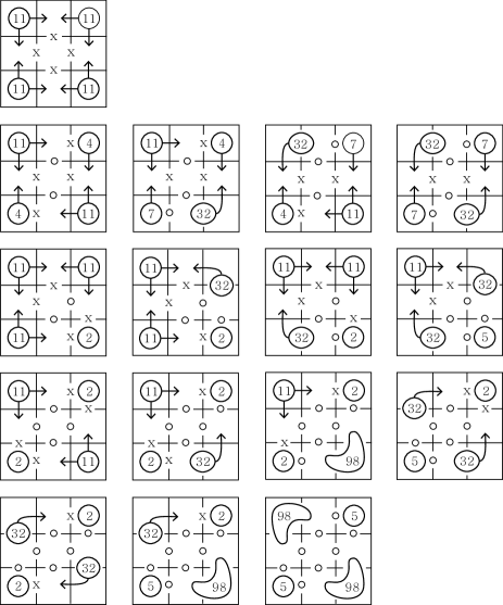
Figure 4. All possible $(3,3)$-quasimosaics from four groups according to the presences of connection points at $a_{1}a_{2}a_{3}a_{4}$ where the four groups are drawn at the first, the second, the third and the last two rows, respectively.

Lastly consider the case of $a_{1}a_{2}a_{3}a_{4}=$ oooo as in the last two rows in the figure. When $b_{1}b_{4}b_{5}b_{8}=$ xxxx, xxxo (and similarly for xxox, xoxx or oxxx), xxoo (and similarly for ooxx), xoox (and similarly for oxxo), xoxo (and similarly for oxox), xooo (and similarly for oxoo, ooxo or ooox) and oooo, $(M_{22},M_{24},M_{42},M_{44})$ has type $(P_{7},P_{1},P_{1},P_{7})$, $(P_{7},P_{1},P_{1},P_{8})$, $(P_{7},P_{1},P_{1},P_{9})$, $(P_{8},P_{1},P_{2},P_{8})$, $(P_{8},P_{1},P_{1},P_{8})$, $(P_{8},P_{1},P_{2},P_{9})$ and $(P_{9},P_{2},P_{2},P_{9})$ respectively. These sixteen occasions produce $(11^{2}\cdot 2^{2}+4\cdot 32\cdot 11\cdot 2^{2}+2\cdot 98\cdot 11\cdot 2^{2}+2\cdot 32^{2}\cdot 5\cdot 2+2\cdot 32^{2}\cdot 2^{2}+4\cdot 98\cdot 32\cdot 5\cdot 2+98^{2}\cdot 5^{2})\times 4=1,635,808$ kinds of quasimosaics. We multiplied by 4 because of the four possible choices of mosaic tiles of $M_{33}$ by Choice rule.

By summing all up, we got that the total number of elements of $\mathbb{Q}^{(3,3)}$ is 2,091,977. The following rule is very useful to get knot mosaics from a quasimosaic.

Lemma 5 (Twofold rule).

A $(p,q)$-quasimosaic can be extended to exactly two knot $(p+2,q+2)$-mosaics.

Proof.

A $(p,q)$-quasimosaic can be extended to knot $(p+2,q+2)$-mosaics by adjoining proper mosaic tiles surrounding it, called boundary mosaic tiles. Since each mosaic tile has even number of connection points, suitable connectedness guarantee that this $(p,q)$-quasimosaic has exactly even number of connection points on its boundary. To make a knot $(p+2,q+2)$-mosaic, all these connection points must be connected pairwise via mutually disjoint arcs when we adjoin boundary mosaic tiles. There are exactly two ways to do as illustrated in Figure 5. ∎

Figure 5. Twofold rule

Finally we get $D_{5,5}=4,183,954$ which is twice of the total number of elements of $\mathbb{Q}^{(3,3)}$ by Twofold rule.

4. Partition matrices

A partition matrix $\mathbb{P}^{(p,q)}$ for the set $\mathbb{Q}^{(p,q)}$ of all $(p,q)$-quasimosaics is a $2^{q}\times 2^{p}$ matrix $(N_{ij})$ where every row (or column) is related to the presence of connection points on the $q$ bottom (or $p$ rightmost, respectively) edges. Roughly speaking, each $N_{ij}$ is the number of all $(p,q)$-quasimosaics whose bottom edges and rightmost edges have specific presences of connection points associated to the $i$-th and the $j$-th in some order, respectively.

In this section, we introduce two partition matrices $\mathbb{P}^{(1,2)}$ and $\mathbb{P}^{(2,2)}$ which would play an important role in finding the precise values of $D_{m,n}$ for $m,n=4,5,6$ except $D_{5,5}$. In Section 5. we build $(2,2)$-, $(2,3)$-, $(2,4)$-, $(3,4)$- and $(4,4)$-quasimosaics (but not $(3,3)$-quasimosaics) by using $(1,2)$- and $(2,2)$-quasimosaics investigated in this section. This construction gives the values of $D_{4,4}$, $D_{4,5}$, $D_{4,6}$, $D_{5,6}$ and $D_{6,6}$ (but not $D_{5,5}$).

First we establish a partition matrix $\mathbb{P}^{(1,2)}$ for $\mathbb{Q}^{(1,2)}$. For an $(1,2)$-quasimosaic, we name three boundary edges on the bottom and on the right by $b_{1}$, $b_{2}$ and $r$ as the left figure in Figure 6. A partition matrix $\mathbb{P}^{(1,2)}$ is a $4\times 2$ matrix $(N_{ij})$ where every row is related to $b_{1}b_{2}$ and every column is related to $r$ as follows; $N_{ij}$ is the number of all $(1,2)$-quasimosaics which have the $i$-th $b_{1}b_{2}$ in the order of xx, xo, ox and oo, and the $j$-th $r$ in the order of x and o. For an example, the family of four $(1,2)$-quasimosaics for $N_{12}$ where $b_{1}b_{2}=$ xx and $r=$ o are illustrated on the right in Figure 6. Note that the sum of all entries of $\mathbb{P}^{(1,2)}$ is the number of elements of $\mathbb{Q}^{(1,2)}$.

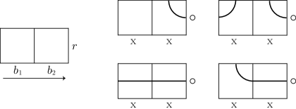
Figure 6. $(1,2)$-quasimosaics and four examples for $N_{12}$ where $b_{1}b_{2}=$ xx and $r=$ o.

Lemma 6.

$$\mathbb{P}^{(1,2)}=\left(\begin{array}[]{cc}4&4\\ 4&10\\ 7&7\\ 7&22\\ \end{array}\right)$$

Proof.

The proof follows from Lemma 4 directly considering types $P_{3}$, $P_{4}$, $P_{5}$ and $P_{6}$. ∎

Next we establish another partition matrix $\mathbb{P}^{(2,2)}$ for $\mathbb{Q}^{(2,2)}$. For an $(2,2)$-quasimosaic, we name four boundary edges on the bottom and on the right by $b_{1}$, $b_{2}$, $r_{1}$ and $r_{2}$, and two interior edges by $c_{1}$ and $c_{2}$ as in Figure 7. A partition matrix $\mathbb{P}^{(2,2)}$ is a $4\times 4$ matrix $(N^{\prime}_{ij})$ where every row is related to $b_{1}b_{2}$ and every column is related to $r_{1}r_{2}$ as follows; $N^{\prime}_{ij}$ is the number of all $(2,2)$-quasimosaics which have the $i$-th $b_{1}b_{2}$, and the $j$-th $r_{1}r_{2}$ in the same order as previous.

Figure 7. $(2,2)$-quasimosaics

Lemma 7.

$$\mathbb{P}^{(2,2)}=\left(\begin{array}[]{cccc}22&22&43&43\\ 22&55&43&139\\ 43&43&109&64\\ 43&139&64&403\\ \end{array}\right)$$

Proof.

Let $M_{*}$ denote the bottom and the right side mosaic tile, and $M_{*}^{c}$ the rest quasimosaic consisting of three mosaic tiles. First, we consider the case $b_{1}r_{1}=$ xx for $N^{\prime}_{11}$, $N^{\prime}_{12}$, $N^{\prime}_{21}$ and $N^{\prime}_{22}$. In this case, $M_{*}^{c}$ always has type $P_{7}$. For every four choices of $b_{2}r_{2}$, the related $c_{1}c_{2}$ has two choices. For example, when $b_{2}r_{2}=$ ox, $c_{1}c_{2}$ must be either ox or xo. Furthermore for each choice of $c_{1}c_{2}$, $M_{*}$ is uniquely determined by Choice rule, except when $b_{2}r_{2}=$ oo and $c_{1}c_{2}=$ oo. $M_{*}$ in the exceptional case has four choices of mosaic tiles. Thus we get $N^{\prime}_{11}$, $N^{\prime}_{12}$, $N^{\prime}_{21}=11\times 2$ and $N^{\prime}_{22}=11+11\times 4$.

Next, consider the case $b_{1}r_{1}=$ xo for $N^{\prime}_{13}$, $N^{\prime}_{14}$, $N^{\prime}_{23}$ and $N^{\prime}_{24}$. Similarly for every four choices of $b_{2}r_{2}$, the related $c_{1}c_{2}$ has two choices. In this case, $M_{*}^{c}$ has type $P_{7}$ if $c_{1}=$ x, and type $P_{8}$ if $c_{1}=$ o. For each choice of $c_{1}c_{2}$, $M_{*}$ is uniquely determined, except when $b_{2}r_{2}=$ oo and $c_{1}c_{2}=$ oo, implying that $M_{*}$ has four choices. Thus we get $N^{\prime}_{13}$, $N^{\prime}_{14}$, $N^{\prime}_{23}=11+32$ and $N^{\prime}_{24}=11+32\times 4$. The case $b_{1}r_{1}=$ ox for $N^{\prime}_{31}$, $N^{\prime}_{32}$, $N^{\prime}_{41}$ and $N^{\prime}_{42}$ will be handled in the same manner.

Finally, consider the case $b_{1}r_{1}=$ oo for the rest four entries of $\mathbb{P}^{(2,2)}$. In this case, $M_{*}^{c}$ possibly has three types $P_{7}$, $P_{8}$ $P_{9}$ according to $c_{1}c_{2}$. And $M_{*}$ is uniquely determined, except when $b_{2}r_{2}c_{1}c_{2}=$ oooo. Thus we get $N^{\prime}_{33}=11+98$, $N^{\prime}_{34}=32\times 2$, $N^{\prime}_{43}=32\times 2$ and $N^{\prime}_{44}=11+98\times 4$. ∎

5. Proof of Theorem 3

In this section, we apply partition matrices $\mathbb{P}^{(1,2)}$ and $\mathbb{P}^{(2,2)}$ to find the precise values of $D_{m,n}$ for $m,n=4,5,6$, except $D_{5,5}$. For a matrix $\mathbb{P}=(N_{ij})$, $\|\mathbb{P}\|$ denote the sum of all entries of $\mathbb{P}$, and $[\mathbb{P}]^{2}=(N_{ij}^{2})$.

Note that $\|\mathbb{P}^{(p,q)}\|$ is the total number of elements of $\mathbb{Q}^{(p,q)}$ for $(p,q)=(1,2)$ or $(2,2)$. Furthermore each element of $\mathbb{Q}^{(p,q)}$ can be extended to exactly two knot $(p+2,q+2)$-mosaics by Twofold rule. Conversely, every knot $(p+2,q+2)$-mosaics can be obtained by extending a proper $(p,q)$-quasimosaic in $\mathbb{Q}^{(p,q)}$. Thus we can conclude $D_{m,n}=2\,\|\mathbb{P}^{(m-2,n-2)}\|$. So $D_{4,4}=2\,\|\mathbb{P}^{(2,2)}\|=2594$.

5.1. Partition matrix multiplying argument

Let $\mathbb{P}^{(1,2)}=(N_{ij})$ and $\mathbb{P}^{(2,2)}=(N^{\prime}_{ij})$. Consider a $(2,3)$-quasimosaic $Q$ in $\mathbb{Q}^{(2,3)}$. We name three boundary edges on the bottom by $b_{1}$, $b_{2}$ and $r^{\prime}$ as upper figures in Figure 8. Let $Q_{l}$ and $Q_{r}$ be the $(2,2)$-quasimosaic obtained from the left two columns of $Q$ and the $(2,1)$-quasimosaic obtained from the rightmost column, respectively. We name again two boundary edges of $Q_{l}$ on the right by $r_{1}$ and $r_{2}$, and other two boundary edges of $Q_{r}$ on the left by $b^{\prime}_{1}$ and $b^{\prime}_{2}$. Then $r_{1}r_{2}$ of $Q_{l}$ must be the same as $b^{\prime}_{1}b^{\prime}_{2}$ of $Q_{r}$. Remark that $Q_{l}$ is an element of $\mathbb{Q}^{(2,2)}$ and $Q_{r}$, after rotating $90^{\circ}$ counter-clockwise, is an element of $\mathbb{Q}^{(1,2)}$. $N_{ik}$ is the number of elements of $\mathbb{Q}^{(2,2)}$ which have the $i$-th $b_{1}b_{2}$ and the $k$-th $r_{1}r_{2}$ in the order of xx, xo, ox and oo, and $N^{\prime}_{kj}$ is the number of elements of $\mathbb{Q}^{(1,2)}$ which have the $k$-th $b^{\prime}_{1}b^{\prime}_{2}$ in the order of xx, xo, ox and oo, and the $j$-th $r^{\prime}$ in the order of x and o. Thus $\sum^{4}_{k=1}N_{ik}N^{\prime}_{kj}$ is the number of elements of $\mathbb{Q}^{(2,3)}$ which have the $i$-th $b_{1}b_{2}$ and the $j$-th $r^{\prime}$. Indeed it is the $i$-th row and the $j$-th column entry of $\mathbb{P}^{(2,2)}\cdot\mathbb{P}^{(1,2)}$. This implies that $\|\mathbb{P}^{(2,2)}\cdot\mathbb{P}^{(1,2)}\|$ is the total number of $\mathbb{Q}^{(2,3)}$. Now we conclude that $D_{4,5}=2\,\|\mathbb{P}^{(2,2)}\cdot\mathbb{P}^{(1,2)}\|=54,226$.

Next, consider a $(2,4)$-quasimosaic $Q^{\prime}$ in $\mathbb{Q}^{(2,4)}$. We name four boundary edges on the bottom by $b_{1}$, $b_{2}$, $r^{\prime}_{2}$ and $r^{\prime}_{1}$ as lower figures in Figure 8. Let $Q^{\prime}_{l}$ and $Q^{\prime}_{r}$ be the $(2,2)$-quasimosaics obtained from the left two columns of $Q^{\prime}$ and from the right two columns, respectively. We name again four boundary edges of $Q^{\prime}_{l}$ and $Q^{\prime}_{r}$ as previous. Again $r_{1}r_{2}$ of $Q^{\prime}_{l}$ must be the same as $b^{\prime}_{1}b^{\prime}_{2}$ of $Q^{\prime}_{r}$. Remark that $Q^{\prime}_{l}$ and $Q^{\prime}_{r}$ is elements of $\mathbb{Q}^{(2,2)}$. Similarly we rotate $Q^{\prime}_{r}$ $90^{\circ}$ counter-clockwise. Thus $\sum^{4}_{k=1}N_{ik}N_{kj}$ is the number of elements of $\mathbb{Q}^{(2,4)}$ which have the $i$-th $b_{1}b_{2}$ and the $j$-th $r^{\prime}_{1}r^{\prime}_{2}$. This implies that $D_{4,6}=2\,\|\mathbb{P}^{(2,2)}\cdot\mathbb{P}^{(2,2)}\|=1,144,526$.

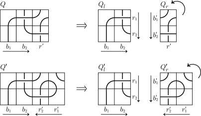
Figure 8. Dividing a $(2,3)$-quasimosaic and a $(2,4)$-quasimosaic into $(2,1)$-quasimosaics and $(2,2)$-quasimosaics.

5.2. Partition matrix squaring argument

Let $\mathbb{P}^{(2,2)}\cdot\mathbb{P}^{(1,2)}=(N_{ij})$. Consider a $(4,3)$-quasimosaic $Q$ in $\mathbb{Q}^{(4,3)}$. We name three interior edges on the middle by $b_{1}$, $b_{2}$ and $r$ as upper figures in Figure 9. Let $Q_{u}$ and $Q_{l}$ be the $(2,3)$-quasimosaics obtained from the upper two rows of $Q$ and from the lower two rows, respectively. We name again three boundary edges of $Q_{u}$ on the bottom by $b^{\prime}_{1}$, $b^{\prime}_{2}$ and $r^{\prime}$, and other three boundary edges of $Q_{l}$ on the top by $b^{\prime\prime}_{1}$, $b^{\prime\prime}_{2}$ and $r^{\prime\prime}$, so that $b^{\prime}_{1}b^{\prime}_{2}r^{\prime}=b^{\prime\prime}_{1}b^{\prime\prime}_{2}r^{\prime\prime}$. We reflect $Q_{l}$ through a horizontal line. Remark that $Q_{u}$ and $Q_{l}$ is elements of $\mathbb{Q}^{(2,3)}$. $N_{ij}$ is the number of elements of $\mathbb{Q}^{(2,3)}$ which have the $i$-th $b^{\prime}_{1}b^{\prime}_{2}$ and the $j$-th $r^{\prime}$. Thus $N_{ij}^{2}$ is the number of elements of $\mathbb{Q}^{(4,3)}$ which have the $i$-th $b_{1}b_{2}$ and the $j$-th $r$. This implies that $D_{5,6}=D_{6,5}=2\,\|[\mathbb{P}^{(2,2)}\cdot\mathbb{P}^{(1,2)}]^{2}\|=331,745,962$.

Now let $\mathbb{P}^{(2,2)}\cdot\mathbb{P}^{(2,2)}=(N_{ij})$. Consider a $(4,4)$-quasimosaic $Q$ in $\mathbb{Q}^{(4,4)}$. We name four interior edges on the middle by $b_{1}$, $b_{2}$, $r_{2}$ and $r_{1}$ as lower figures in Figure 9. The similar argument as previous guarantees that $N_{ij}^{2}$ is the number of elements of $\mathbb{Q}^{(4,4)}$ which have the $i$-th $b_{1}b_{2}$ and the $j$-th $r_{1}r_{2}$. This implies that $D_{6,6}=2\,\|[\mathbb{P}^{(2,2)}\cdot\mathbb{P}^{(2,2)}]^{2}\|=101,393,411,126$.

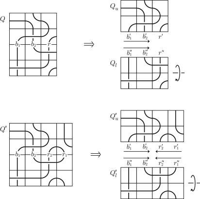
Figure 9. Dividing a $(4,3)$-quasimosaic and a $(4,4)$-quasimosaic into $(2,3)$-quasimosaics and $(2,4)$-quasimosaics, respectively.

6. Conclusion

In this paper, we found the cardinality of knot $(m,n)$-mosaics $D_{m,n}$ for $m,n=4,5,6$. Mainly we build sets of quasimosaics of nine types to calculate two partition matrices related to $(1,2)$- and $(2,2)$-quasimosaics. These partition matrices turn out to be remarkably efficient to count small knot mosaics, even though $D_{m,n}$ increases rapidly so that $D_{6,6}$ is larger than $10^{11}$. In Section 5. we introduce partition matrix multiplying argument and squaring argument to find $D_{m,n}$ for only $m,n=4,5,6$ from these two partition matrices. Eventually, if we have partition matrices for bigger quasimosaics, then we can find the values of $D_{m,n}$ for larger $m,n$ by applying the arguments here. For example, partition matrices for $(1,3)$-, $(2,3)$- and $(3,3)$-quasimosaics is enough to calculate $D_{m,n}$ for $m,n=4,5,6,7,8$. Finding these partition matrices for bigger quasimosaics are worthy of further research.

Recently the authors [2] constructed an algorithm producing $D_{m,n}$ for positive $m,n\geq 2$ by using a recurrence relation of matrices which are called state matrices. State matrices are a generalized version of partition matrices.

References

- [1] K. Hong, H. Lee, H. J. Lee and S. Oh, Upper bound on the total number of knot -mosaics, arXiv:1303.7044.
- [2] K. Hong, H. Lee, H. J. Lee and S. Oh, Quantum knots and the number of knot mosaics, in preperation.
- [3] V. Jones, A polynomial invariant for links via von Neumann algebras, Bull. Amer. Math. Soc. 129 (1985) 103–112.
- [4] V. Jones, Hecke algebra representations of braid groups and link polynomials, Ann. Math. 126 (1987) 335–338.
- [5] L. Kauffman, Knots and Physics (3rd edition), World Scientific Publishers (2001).
- [6] L. Kauffman, Quantum computing and the Jones polynomial, in Quantum Computation and Information, AMS CONM 305 (2002) 101–137.
- [7] T. Kuriya and O. Shehab, The Lomonaco-Kauffman conjecture, J. Knot Theory Ramifications 23 (2014) 1450003.
- [8] H. J. Lee, K. Hong, H. Lee and S. Oh, Mosaic number of knots, arXiv:1301.6041.
- [9] S. Lomonaco (ed.), Quantum Computation, Proc. Symposia Appl. Math. 58 (2002) 358 pp.
- [10] S. Lomonaco and L. Kauffman, Quantum knots, in Quantum Information and Computation II, Proc. SPIE (2004) 268–284.
- [11] S. Lomonaco and L. Kauffman, A 3-Stranded Quantum Algorithm for the Jones Polynomial, Proc. SPIE 6573 (2007) 1–13.
- [12] S. Lomonaco and L. Kauffman, Quantum knots and mosaics, Quantum Inf. Process. 7 (2008) 85–115.
- [13] S. Lomonaco and L. Kauffman, Quantum knots and lattices, or a blueprint for quantum systems that do rope tricks, Proc. Symposia Appl. Math. 68 (2010) 209–276.
- [14] S. Lomonaco and L. Kauffman, Quantizing knots and beyond, in Quantum Information and Computation IX, Proc. SPIE 8057 (2011) 1–14.
- [15] P. Shor and S. Jordan, Estimating Jones polynomials is a complete problem for one clean qubit, Quantum Inform. Comput. 8 (2008) 681–714.