Constrained information transmission on Erdös-Rényi graphs

Abstract

We model the transmission of information of a message on the Erdös-Rényi random graph with parameters $(n,p)$ and limited resources. The vertices of the graph represent servers that may broadcast a message at random. Each server has a random emission capital that decreases by one at each emission. We examine two natural dynamics: in the first dynamics, an informed server performs all its attempts, then checks at each of them if the corresponding edge is open or not; in the second dynamics the informed server knows a priori who are its neighbors, and it performs all its attempts on its actual neighbors in the graph. In each case, we obtain first and second order asymptotics (law of large numbers and central limit theorem), when $n\to\infty$ and $p$ is fixed, for the final proportion of informed servers.
Keywords: information transmission, rumor, labelled trees, Erdös-Rényi random graph
AMS 2000 subject classifications: Primary 90B30; secondary 05C81, 05C80, 60F05, 60J20, 92D30

¹Université Paris Diderot – Paris 7, Mathématiques, case 7012, F–75205 Paris Cedex 13, France
e-mail: comets@math.univ-paris-diderot.fr

²Department of Statistics, Institute of Mathematics, Statistics and Scientific Computation, University of Campinas – UNICAMP, rua Sérgio Buarque de Holanda 651, 13083–859, Campinas SP, Brazil
e-mails: {gallesco,popov,marinav}@ime.unicamp.br

1 Introduction

Information transmission with limited resources on a general graph is a natural problem which appears in various contexts and attracts an increasing interest. Consider a finite graph, each vertex will be seen as a server with a finite resource (e.g., operating battery) given by an independent random variable $K$. Initially a message comes to one of the servers, which will recast the message to its neighbors in the graph as long as its battery allows. In turn, each neighbor starts to emit as soon as it receives the message, and so on, in an asynchronous mode. The transmission stops at a finite time because of the resource constraint. A quantity of paramount interest is the final number of informed servers, i.e., of servers which ever receive the message.

Rumor models deal with ignorant individual (who ignore the rumor), spreaders (who know the rumor and propagates it) and stiflers (who refuse to propagate it) in a population of fixed – but large – size. Two important models, usually presented in continuous time, are well-known: the Maki-Thompson model [21], and the Daley-Kendall model [10] for which the number of eventual knowers obeys a law of large numbers [24] and is asymptotically normal [23] (recently, a large deviations principle for the Maki-Thompson model was also obtained in [18]). Such results extend to a larger family of processes [19] using weak convergence theory for Markov processes. Though we focus here on mean-field type models, we just mention that lattice models lead to different questions [3, 6, 14]. On the other hand, it is well understood that the scaling limit of mean-field models are models on Galton-Watson trees, cf. [1, 5, 7]. Rumor spreading models are alike epidemics propagation models, e.g. frog models [2, 8, 11, 15], and the famous SIR (Susceptible, Infected, Recovered) model which has motivated a number of research papers. See [9] for a survey.

The analysis of random graphs has recently seen a remarkable development [4, 16]. Such graphs yield a natural framework for rumor spreading and epidemic dissemination with more realistic applications to human or biological world [22]. Then, due to lack of homogeneity, setting the threshold concept on firm grounds is already a difficult problem [17], and the literature is abundant in simulation experiments but poor in rigorous results. On the Erdös-Rényi graph, the authors in [12] prove that the time needed for complete transmission in the push protocol (a synchronous dynamics without constraints) is equivalent to that of the complete graph [13] provided that the average degree is significantly larger than $(\ln n)$. In general, it is reasonable to look for quantitative results from perturbations of the homogeneous case. From the point of view of applications, the graph may be thought of as a wireless network, the vertices of which are battery-powered sensors with a limited energy capacity. The reader will find in Sect.1 of [7] a discussion of applications to the performance evaluation of information transmission in wireless networks.

On the complete graph, the process can be reduced by homogeneity to a Markov chain in the quadrant with absorption on the axis, as recalled in the forthcoming Section 2.1. For a random graph, fluctuations of the vertex degrees create inhomogeneities which make the above description non-Markovian and computations intractable. This can be already seen in the simplest example, the Erdös-Rényi graph. Homogeneity is present, not in the strict sense but in a statistical one, and independence is deeply rooted in its construction. From many perspectives, this random graph with fixed positive $p$ has been proved to be very similar to the complete graph as $n$ becomes large. In the present paper we show that the information transmission process on this random graph is a bounded perturbation of that on the complete graph with appropriate resource distribution. We will use the above mentioned similarities to construct couplings between information process with constraints on the complete graph and on the Erdös-Rényi graph. Then we control the discrepancy between the two models and its propagation as the process evolves.

In this paper, we consider two natural dynamics of the information transmission process on the Erdös-Rényi graph:

• (i) an informed server performs $K$ attempts by choosing a server at random independently at each attempts, then checks for each of them if the corresponding edge is open or not;

• (ii) the informed server knows a priori who are its neighbors, and it performs all its $K$ attempts on the set of its actual neighbors in the graph.

First of all we prove the existence of a threshold: Transmission takes place at a macroscopic level if and only if $p{\mathbb{E}}K>1$ in the case (i), and iff ${\mathbb{E}}K>1$ in the case (ii). Then, with positive probability, a positive proportion of servers will be informed, whereas in the case of the reverse inequalities, the final number of informed servers is bounded in probability. The value of the threshold is natural, observing that, in the first case, attempts taking place on closed edges are lost, so that the effective number of attempts is close (as $N$ increases) to a random sum

$$\widehat{K}=\sum_{1\leq k\leq K}B_{k}$$ (1)

with $(B_{k},k\geq 1)$ i.i.d. Bernoulli with parameter $p$.

Our main results, Theorems 2.1, 2.2, 2.3 and 2.4 below, are the laws of large numbers and the central limit theorems for the number of informed servers with explicit values of the limits in each case. Our approach is to show that, in the limit $n\to{\infty}$ with a fixed $p\in(0,1]$, the information transmission process on the Erdös-Rényi graph is shown to be a bounded perturbation of the process on the complete graph with a suitable resource law. Then, the first and second order asymptotics, obtained by explicit computations on the complete graph in [20, 7], still hold on the random graph.

An important property of the model is abelianity, e.g. see Proposition 4.4. We can change the order in which emitters are taken without changing the law of the final state of the process, and construct an efficient coupling of the processes on the two graphs. This property also implies that assuming the servers emit in a burst does not change the final result ( a nice feature of the burst emission assumption is that it reveals a branching structure). The two dynamics we consider here are simple and reasonable protocols, but we don’t make any attempt for generality in this paper. We will use an exploration process which allows to reveal at each step, only the necessary part of the graph in order to preserve randomness and stationarity in the subsequent steps.

Outline of the paper: In Section 2 we define the model, recall useful results for the complete graph, and state our main results. Then, labeled trees are introduced with a view towards our constructions. Section 4 contains the proofs in the case of the first dynamics (i), and the last section deals with dynamics (ii).

2 Model and results

We start to recall some results for the information transmission process on the complete graph.

2.1 Known asymptotics in the case of the complete graph

When any server is connected to any other one, the communication network is the complete graph on ${\cal N}=\{1,\ldots,n\}$. We consider here discrete time and we scale the time so that there is exactly one emission per time unit. Then, the information process can be fully described by the number $N_{n}(s)$ of informed servers at time $s$ and the number $S_{n}(s)$ of available emission attempts (see [7] for the formal definition). Precisely, for the information process with resource $K$ on the complete graph, the pair $(S_{n}(s),N_{n}(s))_{s=0,1,\ldots}$ on ${\mathbb{Z}}_{+}\times[1,n]$ is a Markov chain with transitions

$$\left\{\begin{array}[]{rcl}{\mathbb{P}}\Big{(}S_{n}(s\!+\!1)=S_{n}(s)\!-\!1,N_{n}(s\!+\!1)=N_{n}(s)\mid\mathcal{F}_{s}\Big{)}&=&\frac{N_{n}(s)}{n},\\ {\mathbb{P}}\Big{(}S_{n}(s\!+\!1)=S_{n}(s)\!+\!k\!-\!1,N_{n}(s\!+\!1)=N_{n}(s)\!+\!1\mid\mathcal{F}_{s}\Big{)}&=&\left(1-\frac{N_{n}(s)}{n}\right){\mathbb{P}}(K=k),\end{array}\right.$$ (2)

for $k\geq 0,$ with $\mathcal{F}_{s}$ the $\sigma$-field generated by $S_{n}(\cdot)$ and $N_{n}(\cdot)$ on $[0,s]$. The transition probabilities are easily understood by interpreting what can occur at a given step: On the first line of (2) the emission takes place towards a previously informed target, though in the second one the target yields its own resource (a fresh r.v. $K$). The chain is absorbed in the vertical semi-axis, at the finite time ${\mathfrak{T}}_{n}=\inf\{s:S_{n}(s)=0\}$.

In this section we recall some results from [7] (and of [20] for constant $K=2$) on the first and second order asymptotics of $N_{n}({\mathfrak{T}}_{n})=N_{n}({\infty})$. Let $q\in[0,1)$ be the largest root of

$$q\;{\mathbb{E}}K+\ln(1-q)=0.$$ (3)

Then, $0<q<1$ for ${\mathbb{E}}K>1$ and $q=0$ if ${\mathbb{E}}K\leq 1$.

Theorem A ([7], Theorems 2.2 and 2.3).

(i) Assume ${\mathbb{E}}K\in(0,{\infty})$. Then, as $n\to{\infty}$,

$$\frac{1}{n}N_{n}({\mathfrak{T}}_{n})\stackrel{{\scriptstyle\text{\tiny law}}}{{\longrightarrow}}q\times Ber(\sigma^{GW})$$

with $Ber(\sigma)$ a Bernoulli variable with parameter $\sigma$, and $\sigma^{GW}$ is the largest solution $\sigma\in[0,1]$ of

$$1-\sigma={\mathbb{E}}\left[(1-\sigma)^{K}\right],$$ (4)

i.e. the survival probability of a Galton-Watson process with reproduction law $K$.

(ii) Assume ${\mathbb{E}}K>1$ and ${\mathbb{E}}K^{2}<{\infty}$. Denote by $\sigma_{K}^{2}$ the variance of $K$ and fix some $\varepsilon$ with $0<\varepsilon<-\ln(1-q)$. As $n\to{\infty}$, we have the convergence in law, conditionally on $\{{\mathfrak{T}}_{n}\geq\varepsilon n\}$,

$$n^{-1/2}\big{(}N_{n}({\mathfrak{T}}_{n})-nq\big{)}\stackrel{{\scriptstyle\text{\tiny law}}}{{\longrightarrow}}{\mathcal{N}}(0,\sigma_{q}^{2}),$$

with ${\mathcal{N}}(0,\sigma^{2})$ a centered Gaussian with variance $\sigma^{2}$, and

$$\sigma_{q}^{2}=\frac{q\sigma_{K}^{2}(1-q)^{2}+q(1-q)+(1-q)^{2}\ln(1-q)}{[(1-q){\mathbb{E}}K-1]^{2}}\color[rgb]{0,0,0}>0.\color[rgb]{0,0,0}$$ (5)

We now state the main results of this paper, i.e. when the connection network is the Erdös-Rényi graph $G(n,p)$. Now, a server starting to emit, instantaneously exhausts its $K$ emissions in a burst. The time unit corresponds to complete exhaustion for an emitter. Let $N_{n}^{er}(t)$ be the number of informed servers at time $t$.

2.2 First mode of transmission on the Erdös-Rényi graph

First of all, the Erdös-Rényi graph $G(n,p)$ is sampled on the vertex set $\cal N$ (each unoriented edge is kept independently with probability $p$ or removed with probability $1-p$), and one vertex is selected as the first informed server. Then, at each integer time, an informed server which is not yet exhausted is selected to emit its $K$ attempts in a burst. For each attempt a target in $\cal N$ is selected (in the full population including the emitter). If the target is already informed or if the corresponding edge is not in the graph, the attempt is lost. Otherwise, the target becomes informed. After all attempts are checked, the emitter is turned to exhausted and the time is increased by one unit. The transmission ends at a finite time $\tau_{n}^{er}$, which is the first time when all informed servers are exhausted.

Note that, because of the burst emission here, the time scale is different from Section 2.1 with one emission at a time. With $N_{n}^{er}(t)$ the number of informed servers at time $t$, we are interested in the asymptotics of

$$\tau_{n}^{er}=N_{n}^{er}(\tau_{n}^{er})=N_{n}^{er}({\infty}).$$

The first equality holds since it takes one time unit to exhaust an informed server, and the last one holds since the process stops at $\tau_{n}^{er}$.

We will encounter the above quantities when $K$ is replaced by $\widehat{K}$ from (1), that we will denote using the same symbol with a hat: In particular, $\widehat{\theta}=0=\widehat{\sigma}^{GW}$ if $p{\mathbb{E}}K\leq 1$, and for $p{\mathbb{E}}K>1,\widehat{q}\in(0,1)$ is the positive root of

$$\widehat{q}p{\mathbb{E}}K+\ln(1-{\widehat{q}})=0,$$ (6)

and $\widehat{\sigma}^{GW}$ is the positive root of

$$1-\widehat{\sigma}^{GW}={\mathbb{E}}\left[(1-\widehat{\sigma}^{GW})^{\widehat{K}}\right]={\mathbb{E}}\left[(1-p\widehat{\sigma}^{GW})^{K}\right],$$

that is, equation (4) with hats.

Theorem 2.1.

Assume ${\mathbb{E}}K^{2}<{\infty}$. Then,

$$\frac{\tau_{n}^{er}}{n}\stackrel{{\scriptstyle\text{\tiny law}}}{{\longrightarrow}}\widehat{q}\times Ber(\widehat{\sigma}^{GW})\;.$$

The interesting case is of course when ${\mathbb{E}}\widehat{K}=p{\mathbb{E}}K>1$ to have $\widehat{\sigma}^{GW}>0$. In this case, let also

$$\widehat{\sigma}_{{\color[rgb]{0,0,0}\hat{q}}}^{2}=\frac{\widehat{q}\sigma_{\widehat{K}}^{2}(1-\widehat{q})^{2}+\widehat{q}(1-\widehat{q})+(1-\widehat{q})^{2}\ln(1-\widehat{q})}{[(1-\widehat{q})p{\mathbb{E}}K-1]^{2}}{\color[rgb]{0,0,0}>0},$$

with $\sigma_{\widehat{K}}^{2}=p(1-p){\mathbb{E}}K+p^{2}\sigma_{K}^{2}$ the variance of $\widehat{K}$.

Theorem 2.2.

Assume ${\mathbb{E}}K^{2}<{\infty}$ and $p{\mathbb{E}}K>1$. Fix $\varepsilon\in(0,\widehat{q})$. Then, conditionally on $\{\tau^{er}_{n}>n\varepsilon\}$, we have convergence in law:

$$\frac{\tau_{n}^{er}-n\widehat{q}}{\sqrt{n}}\stackrel{{\scriptstyle\text{\tiny law}}}{{\longrightarrow}}{\mathcal{N}}(0,\widehat{\sigma}_{{\color[rgb]{0,0,0}\hat{q}}}^{2})\;.$$

2.3 Main results for the second mode of transmission

Again, we start by sampling the Erdös-Rényi graph $G(n,p)$ and one vertex as the first informed server. Then, at each integer time, an informed server which is not yet exhausted is selected to emit its $K$ attempts in a burst, each attempt being towards a random target uniformly distributed among the neighbors in the graph. (If a site has no neighbours, it wastes its resource without result, and after that the process continues.) If the target is already informed the attempt is lost, but otherwise the target becomes informed. After all attempts are checked, the emitter is turned to exhausted and the time is increased by one unit. The transmission ends at some finite time $\bar{\tau}_{n}^{er}$, with $\bar{\tau}_{n}^{er}$ informed servers. In the following theorems $q$, $\sigma^{GW}$ and $\sigma_{q}$ are from Section 2.1.

Theorem 2.3.

Assume ${\mathbb{E}}K^{2}<{\infty}$.

$$\frac{\bar{\tau}^{er}_{n}}{n}\stackrel{{\scriptstyle\text{\tiny law}}}{{\longrightarrow}}q\times Ber(\sigma^{GW}).$$

Theorem 2.4.

Assume ${\mathbb{E}}K^{2}<{\infty}$ and ${\mathbb{E}}K>1$. Fix $\varepsilon\in(0,q)$. Then, conditionally on $\{\bar{\tau}^{er}_{n}>n\varepsilon\}$, we have convergence in law:

$$\frac{\bar{\tau}^{er}_{n}-nq}{\sqrt{n}}\stackrel{{\scriptstyle\text{\tiny law}}}{{\longrightarrow}}{\mathcal{N}}(0,\sigma_{q}^{2}).$$

2.4 Strategy of the proofs

We use the known results about the information process on the complete graph to derive results on the Erdös-Rényi graph.

We show that case (i) is similar to the complete graph with $\hat{K}$ attempts. The difference is that in the latter model, the Bernoulli random variables in (1) (indicating the presence of the relevant edges) are regenerated independently at each attempt to transmit, though in the former the state of an edge is determined at its first appearance. A coupling argument is made to show that in fact this makes little difference to the final number of vertices receiving the information. In case (ii) we keep track of which edges are in a known state and the key argument is that with high probability only $o(n)$ edges out of a vertex will ever be in a known state. Hence the argument is to show that, most likely, there will be $O_{P}(1)$ transmissions in which there is a discrepancy between the models. To take care of the consequences of discrepancies, we delay them until the end of the process – taking advantage of irrelevance of the order of transmission. Finally we show that these few extra transmissions make little difference to the final proportion of vertices receiving the information.

3 Construction from labelled trees

3.1 Labelled trees

Let $\mathcal{W}=\cup_{m\geq 0}{\mathbb{N}}^{m}$ be the set of all finite words on the alphabet ${\mathbb{N}}=\{1,2,\dots\}$. By convention ${\mathbb{N}}^{0}=\{\o\}$ contains only one element which can be interpreted as the empty word and which, in our formalism, will be the root of the tree. An element of $\mathcal{W}$ different from $\o$ is thus a $m$-uple $u=(i_{1},\dots,i_{m})$ which, to simplify, will be denoted by $u=i_{1}\dots i_{m}$. The length of $u$ denoted by $|u|$ equals $m$ (with $|\o|=0$). If $j\in{\mathbb{N}}$, we denote by $uj$ the element $i_{1}\dots i_{m}j$. The elements of the form $uj$ are interpreted as the descendants of $u$. We will use the following total order relation on $\mathcal{W}$, we write $w\leq w^{\prime}$ if: $|w|<|w^{\prime}|$, or $|w|=|w^{\prime}|$ and $w\leq_{lex}w^{\prime}$ in the lexicographical order.

A rooted tree $\mathcal{T}$ is an undirected simple connected graph without cycles and with a distinguished vertex. A labelled tree $(\mathcal{T},L)$ is a rooted tree $\mathcal{T}$ equipped with a label mapping $L$ from $\mathcal{T}$ to some set $\mathcal{N}$. Labelled trees we will consider are connected subsets of $\mathcal{W}$ containing $\o$. The label set $\mathcal{N}=\{1,2,\ldots,n\}$ encodes the set of servers. For the sake of brevity, we use the short notation $Lv=L(v)$, that the reader will distinguish from concatenation.

3.2 Construction and coupling

Let $n\geq 2$ and $\mathcal{N}=\{1,\dots,n\}$. On a suitable probability space $(\Omega,\mathcal{F},{\mathbb{P}})$, we define the following independent random elements:

• $(K_{i})_{i\in\mathcal{N}}$ are i.i.d. non-negative integer random variables;

• $I_{0}$ is a uniform random variable on $\mathcal{N}$;

• $(I^{i}_{k})_{(i,k)\in\mathcal{N}\times{\mathbb{N}}}$ are independent uniform random variables on $\mathcal{N}$;

• $({B}^{i}_{k})_{(i,k)\in\mathcal{N}\times{\mathbb{N}}}$ are independent Bernoulli random variables of parameter $p$.

In the next sections, we construct couplings between different labelled trees using the above random elements. The different trees $\mathcal{T}({\infty})=\lim_{t\nearrow{\infty}}\mathcal{T}(t)$ are limits of some sequence, they will be constructed dynamically discovering step by step their nodes and their labels. At each step $t$, the labels of the tree $\mathcal{T}(t)$ are all different. They represent the informed servers at time $t$ and will be partitioned into two (as in Section 4.1) or three (as in Section 5 and the end of Section 4.2) subsets:

$$\mathcal{T}(t)=\mathcal{A}(t)\cup\mathcal{E}(t)\cup\mathcal{D}(t),\qquad\mathcal{A}(t),\mathcal{E}(t),\mathcal{D}(t)\;{\rm disjoint},$$ (7)

where $\mathcal{E}(t)$ encodes the exhausted servers (those which have already used their resource), $\mathcal{A}(t)$ encodes the active servers (those which are waiting to use their resource and ready to transmit), and $\mathcal{D}(t)$ encodes the set of delayed servers (those which have not started to transmit but are temporarily delayed). In Section 4.1, $\mathcal{D}(t)$ is empty.

Remark 3.1.

The sets in (7) and the mapping $L$ depend on the number $n$ of servers. In general, for the sake of simplicity, we do not indicate explicitly the dependence in the notations.

In the next section, we construct transmission processes on the complete graph with law $\widehat{K}$ and on Erdös–Rényi random graph, using the above elements, thus we have a coupling between these processes, allowing to transfer results from one to the other. The reader may wonder, here or below, why we introduce so many independent r.v.’s in the construction, since a given edge is decided to be open or closed in the Erdös-Rényi graph only once, namely at its first appearance. The reason is that coupling the process with one on the complete graph requires to decide each edge more than once (cf.  Sections 4.1 and 4.2).

4 First mode of emission: Burst emission

We model the transmission of a message on the Erdös-Rényi random graph of parameter $p$. Each vertex $i$ of the graph is a server with resource $K_{i}$. Initially, one vertex receives a message and tries to send it to its neighbors: first it choses, uniformly among all the servers, one server (the target) to which it will try to send the message. If the edge between these two servers is present, then the information is transmitted and otherwise it is not. The emitting server repeats this operation until it has exhausted its own resource $K_{i}$. If the edge is present and the target server already knows the information then the emitter just loses one resource unit. When the emitter has exhausted its resource, we pick a new server among the informed ones and it starts to emit according to the same procedure. The process stops when all the informed servers have exhausted their resources.

4.1 Erdös-Rényi graph

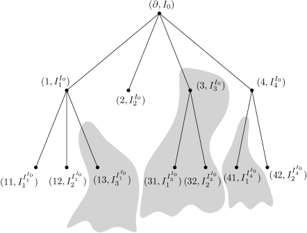
Figure 1: Two first generations of a labeled random tree, with $K_{I_{0}}=4,$ $K_{I_{1}^{I_{0}}}=\leavevmode\nobreak\ 3,K_{I_{2}^{I_{0}}}=0,$ $K_{I_{3}^{I_{0}}}=2,$ and $K_{I_{4}^{I_{0}}}=2$ is represented by the line segments. The other variables used in the construction are: $n=38;I_{0}=23;I^{23}_{1}=12,I^{23}_{2}=7,I^{23}_{3}=12,I^{23}_{4}=30,I^{12}_{1}=18,I^{12}_{2}=I^{12}_{3}=2,I^{30}_{2}=27;B^{23}_{k}=1(1\leq k\leq 4),B^{12}_{1}=B^{12}_{2}=1,B^{12}_{3}=0,B^{30}_{1}=0,B^{30}_{2}=1$. Some parts of the tree, included in the shaded parts, were pruned out, because a label has been already discovered or because an edge is closed in the Erdös-Rényi graph.

We construct dynamically the random labelled tree $\mathcal{T}^{er}(t)$ in the following way. At $t=0$, using $I_{0}$, we discover the label of the root $\o$ and we set $L(\o)=I_{0}$. In the rest of this section, we abbreviate for clarity $L^{er}$ by $L$. Denoting by $i$ the value of $I_{0}$ for short notations, we consider a realization of $K_{i}$, ${B}^{i}_{1},\dots,{B}^{i}_{K_{i}}$ and $I^{i}_{1},\dots,I^{i}_{K_{i}}$. To each descendant $l$, $1\leq l\leq K_{i}$, of the root we associate the label $I^{i}_{l}$. Initially, we define

$$X(0) =\o,$$

$$\mathcal{X}(0) =\{w\in\mathcal{W}:|w|=1,1\leq w\leq K_{i}\},$$

$$\mathcal{X}^{er}(0) =\{w\in\mathcal{W}:|w|=1,1\leq w\leq K_{i},{B}^{i}_{w}=1\},$$

$$L(w) =I^{i}_{w},\qquad w\in\mathcal{X}(0),$$

$$\mathcal{A}^{er}(0) =\{w\in\mathcal{X}^{er}(0):L(w)\neq i,L(w)\neq L(w^{\prime}),w^{\prime}<w,w^{\prime}\in\mathcal{X}(0)\},$$

$$\mathcal{T}^{er}(0) =\{\o\}\cup\mathcal{A}^{er}(0).$$ (8)

With the process $(X(t),\mathcal{T}^{er}(t),\mathcal{A}^{er}(t))$ at time $t$ and $L$ defined on $\mathcal{T}^{er}(t)$, the value at the next step $t+1$ is defined by:

• If $\mathcal{A}^{er}(t)$ is non empty, we let $X(t+1)$ be its first element in the total order $\leq$,

  $$X(t+1)=\inf\{w\in\mathcal{A}^{er}(t)\},\phantom{*}\mbox{denoted by $v$}$$

  and we consider a realization of $K_{Lv}$, ${B}^{Lv}_{1},\dots,{B}^{Lv}_{K_{Lv}}$ and $I^{Lv}_{1},\dots,I^{Lv}_{K_{Lv}}$. To each descendant $vl$, $1\leq l\leq K_{Lv}$ we associate the label $I^{Lv}_{l}$. Then, we update the sets of vertices

  $$\mathcal{X}(t+1) =\{vl\in\mathcal{W}:1\leq l\leq K_{Lv}\},$$

  $$L(w) =I^{Lv}_{l},\qquad w=vl\in\mathcal{X}(t+1),$$

  $$\mathcal{X}^{er}(t+1) =\{vl\in\mathcal{W}:1\leq l\leq K_{Lv},{B}^{Lv}_{l}=1\},$$

  $$\mathcal{A}^{er}(t+1) =(\mathcal{A}^{er}(t)\setminus\{v\})\cup\{w\in\mathcal{X}^{er}(t+1):L(w)\notin L(\mathcal{T}^{er}(t)),$$

  $$\qquad\qquad\qquad L(w)\neq L(w^{\prime}),w^{\prime}<w,w^{\prime}\in\mathcal{X}(t+1)\},$$

  $$\mathcal{T}^{er}(t+1) =\mathcal{T}^{er}(t)\cup\mathcal{A}^{er}(t+1).$$ (9)

• If $\mathcal{A}^{er}(t)$ is empty, we set $\tau_{n}^{er}=t$ and the construction is stopped.

At each step of the construction, we set $\mathcal{E}^{er}(t+1)=\mathcal{E}^{er}(t)\cup\{X(t+1)\}$ starting from $\mathcal{E}^{er}(0)=\{\o\}$, and $\mathcal{D}^{er}(t)\equiv\emptyset$. Hence $v=X(t+1)$ is moved from active to exhausted at time $t+1$, and the partition (7) reduces to two subsets in the case of the Erdös-Rényi graph. ∎

The construction is illustrated by Figure 1.

Remark 4.1.

(i) Note that the definitions of active servers in (8) and (9) require that the label has not appeared before. Indeed the first Bernoulli variable determines the status of the edge.

(ii) Note that $L^{er}$ has been defined in this process on a larger tree than needed. In fact, we consider its restriction to $\mathcal{T}^{er}({\infty})=\mathcal{T}^{er}(\tau_{n}^{er})$, which is indeed injective. This procedure of restriction is needed in all the subsequent constructions.

It is not completely obvious that this construction corresponds to the description given at the beginning of Section 2.2. However, this is the case, as we show now. Here, an edge is open or closed according to the Bernoulli variable used on the first appearance of the edge in the construction. Here is a formal definition. Denote by $\cal E$ the set of unoriented edges on $\cal N$, i.e. the set of $e=\langle i,j\rangle,i,j\in{\cal N}$ (allowing self-edge). We say that the edge $e$ has appeared in the construction if there is some $t\;(0\leq t\leq\tau_{n}^{er}-1)$ and some $\ell\leq K_{L[X(t)]}$ such that

$$e=\langle L[X(t)],L[X(t)\ell]\rangle.$$

We denote by $t(e)$ and $\ell(e)$ the smallest (in the lexicographic order) $t$ and $\ell$ with the above property, by $Ap(t)=\{e:t(e)=t\}$ the set of edges which have appeared at time $t$ and $Ap=\cup_{t\geq 0}Ap(t)$. With an additional i.i.d. Bernoulli($p$) family $({B}^{i}_{-k})_{i\in{\cal N},k\geq 1}$ independent of the variables in (i–iv), define

$$B(e)=\left\{\begin{array}[]{lll}B^{i}_{k}&{\rm if}&e\in Ap,i=L[X(t(e))],k=\ell(e),\\ B^{i}_{-j}&{\rm if}&e\notin Ap,e=\langle i,j\rangle,i\leq j.\end{array}\right.$$

Proposition 4.1.

The family $(B(e),e\in{\cal E})$ is i.i.d. Bernoulli($p$), and is independent of the family $(I^{i}_{k})_{i\in{\cal N},k\geq 1}$,$(K_{i})_{i\in{\cal N}}$, $I_{0}$.

The proposition shows that the above construction coincides with the description of the information transmission process on the Erdös-Rényi graph as given in the beginning of Section 2.2, in which the random graph is defined by the $B(e)$’s, and the dynamics uses the variables $I_{0},I^{i}_{\cdot},K_{i}$. Though the proof is standard, we give it for completeness.

$\Box$ For bounded measurable functions $f_{e},g_{i},h$ defined on the appropriate spaces, we compute

$${\mathbb{E}}\prod_{e\in{\cal E}}f_{e}(B(e))\times\prod_{i\in{\cal N}}g_{i}(K_{i},I^{i}_{\cdot})\times h(I_{0})=\qquad\qquad\qquad\qquad\qquad\qquad\qquad$$

$$\sum_{T,A(\cdot)}{\mathbb{E}}\prod_{e\in{\cal E}}f_{e}(B(e))\times\prod_{i\in{\cal N}}g_{i}(K_{i},I^{i}_{\cdot})\times h(I_{0}){\mathbf{1}}_{\{\tau_{n}^{er}=T,Ap(\cdot)=A(\cdot)\}}$$

where $A(\cdot)=(A(t),t=0,\ldots T-1)$ ranges over the collection of $T$ disjoints subsets of $\cal E$. With $A=\cup_{t}A(t)$, by independence of $({B}^{i}_{-k})_{i,k}$ with the other variables, the expectation in the last term is equal to

$$\Big{(}\prod_{e\notin A}{\mathbb{E}}f_{e}(B(e))\Big{)}\times\Big{(}{\mathbb{E}}\prod_{e\in A}f_{e}(B(e))\times\prod_{i\in{\cal N}}g_{i}(K_{i},I^{i}_{\cdot})\times h(I_{0}){\mathbf{1}}_{\{\tau_{n}^{er}=T,Ap(\cdot)=A\}}\Big{)}.$$ (10)

Let us write the last expectation as

$${\mathbb{E}}\Big{(}\prod_{e\in A(T-1)}f_{e}\big{(}B^{L[X(t(e))]}_{\ell(e)}\big{)}\times\prod_{e\in A\setminus A(T-1)}f_{e}(B(e))\times\prod_{i\in{\cal N}}g_{i}(K_{i},I^{i}_{\cdot})\times h(I_{0}){\mathbf{1}}_{\{\tau_{n}^{er}=T,Ap(\cdot)=A\}}\Big{)}\qquad$$

$$\stackrel{{\scriptstyle\rm indep.}}{{=}}\Big{(}\prod_{e\in A(T-1)}{\mathbb{E}}f_{e}(B(e))\Big{)}\times\Big{(}{\mathbb{E}}\prod_{e\in A\setminus A(T-1)}f_{e}(B(e))\times\prod_{i\in{\cal N}}g_{i}(K_{i},I^{i}_{\cdot})\times h(I_{0}){\mathbf{1}}_{\{\tau_{n}^{er}=T,Ap(\cdot)=A\}}\Big{)}$$

$$\stackrel{{\scriptstyle\rm iterating}}{{=}}\Big{(}\prod_{e\in A}{\mathbb{E}}f_{e}(B(e))\Big{)}\times\Big{(}{\mathbb{E}}\prod_{i\in{\cal N}}g_{i}(K_{i},I^{i}_{\cdot})\times h(I_{0}){\mathbf{1}}_{\{\tau_{n}^{er}=T,Ap(\cdot)=A\}}\Big{)}.\qquad\qquad\qquad\qquad\qquad$$

The first factor in the last term complements the one in (10), and we finally get

$${\mathbb{E}}\prod_{e\in{\cal E}}f_{e}(B(e))\times\prod_{i\in{\cal N}}g_{i}(K_{i},I^{i}_{\cdot})\times h(I_{0})$$**************

$$=\prod_{e\in{\cal E}}{\mathbb{E}}f_{e}(B(e))\Big{(}\sum_{T,A(\cdot)}{\mathbb{E}}\prod_{i\in{\cal N}}g_{i}(K_{i},I^{i}_{\cdot})\times h(I_{0}){\mathbf{1}}_{\{\tau_{n}^{er}=T,Ap(\cdot)=A\}}\Big{)}$$

$$=\prod_{e\in{\cal E}}{\mathbb{E}}f_{e}(B(e))\times\Big{(}{\mathbb{E}}\prod_{i\in{\cal N}}g_{i}(K_{i},I^{i}_{\cdot})\times h(I_{0})\Big{)},$$

by summing over $T,A(\cdot)$. This proves the proposition. ∎

4.2 Complete graph

With the above ingredients, we start to construct the information transmission model on the complete graph according to two different dynamics with distribution $\widehat{K}$. The first construction is simple and natural (and is close to that performed in Section 2.1 of [7]), but the second one makes a useful coupling with the transmission model on the Erdös-Rényi graph.

Sequential construction. We construct dynamically the random tree $\mathcal{T}^{cg,s}(t)$ together with the label mapping $L^{cg,s}$ that we abbreviate for clarity by $L=L^{cg,s}$ in the construction. The exploration vertex $X(t)$ we introduce below, also depends on the dynamics, $X=X^{cg,s}$, but we omit the superscript for the same reason.

At $t=0$, using $I_{0}$, we discover the label of the root, $L(\o)=I_{0}$. Suppose that $I_{0}=i$, and consider the realization of $K_{i}$, ${B}^{i}_{1},\dots,{B}^{i}_{K_{i}}$ and $I^{i}_{1},\dots,I^{i}_{K_{i}}$. The label of each descendant $l$, $1\leq l\leq K_{i}$, of the root is $I^{i}_{l}$. Initially, we suppose

$$X(0) =\o,$$

$$\mathcal{X}^{cg,s}(0) =\{w\in\mathcal{W}:|w|=1,1\leq w\leq K_{i},{B}^{i}_{w}=1\},$$

$$L(w) =I^{i}_{w},\qquad w\in\mathcal{X}^{cg,s}(0),$$

$$\mathcal{A}^{cg,s}(0) =\{w\in\mathcal{X}^{cg,s}(0):L(w)\neq i,L(w)\neq L(w^{\prime}),w^{\prime}<w,w^{\prime}\in\mathcal{X}^{cg,s}(0)\},$$

$$\mathcal{T}^{cg,s}(0) =\{\o\}\cup\mathcal{A}^{cg,s}(0).$$ (11)

With the process $(\mathcal{T}^{cg,s}(t),\mathcal{X}^{cg,s}(t),\mathcal{A}^{cg,s}(t))$ at time $t$, its value at the next step $t+1$ is defined by:

• If $\mathcal{A}^{cg,s}(t)$ is non empty, we let $X(t+1)$ be its first element,

  $$X(t+1)=\inf\{w\in\mathcal{A}^{cg,s}(t)\},\phantom{*}\mbox{denoted by $v$}$$

  and we consider a realization of $K_{Lv}$, ${B}^{Lv}_{1},\dots,{B}^{Lv}_{K_{Lv}}$ and $I^{Lv}_{1},\dots,I^{Lv}_{K_{Lv}}$. To each descendant $vl$, $1\leq l\leq K_{Lv}$ we associate the label $I^{Lv}_{l}$. Then, we update the sets:

  $$\mathcal{X}^{cg,s}(t+1) =\{vl\in\mathcal{W}:1\leq l\leq K_{Lv},{B}^{Lv}_{l}=1\},$$

  $$L(w) =I^{Lv}_{l},\qquad w=vl\in\mathcal{X}^{cg,s}(t+1),$$

  $$\mathcal{A}^{cg,s}(t+1) =(\mathcal{A}^{cg,s}(t)\setminus\{v\})\cup\Big{\{}w\in\mathcal{X}^{cg,s}(t\!+\!1):L(w)\notin L(\mathcal{T}^{cg,s}(t)),$$

  $$\phantom{**************}L(w)\neq L(w^{\prime}),w^{\prime}<w,w^{\prime}\in\mathcal{X}^{cg,s}(t\!+\!1)\Big{\}},$$

  $$\mathcal{T}^{cg,s}(t+1) =\mathcal{T}^{cg,s}(t)\cup\mathcal{A}^{cg,s}(t+1).$$ (12)

• If $\mathcal{A}^{cg,s}(t)$ is empty, we set $\tau_{n}^{cg,s}=t$ and the transmission stops.

At each step of the construction, we set $\mathcal{E}^{cg,s}(t+1)=\mathcal{E}^{cg,s}(t)\cup\{X(t+1)\}$ starting from $\mathcal{E}^{cg,s}(0)=\{\o\}$, and $\mathcal{D}^{cg,s}(t)\equiv\emptyset$, so that the partition (7) reduces again to two subsets. ∎

Remark 4.2.

Observe that the condition “$L(w)\neq L(w^{\prime})$, $w^{\prime}<w$” in the definition of $\mathcal{A}^{cg,s}(t)$ avoids counting twice the same label. We also emphasize that (11)–(12) and (8)–(9) differ by the set $\mathcal{X}^{\cdot}(t)$ for $w^{\prime}$ in the next-to-last line of the formulae. In the Erdös-Rényi construction the same Bernoulli variable is in force each time an edge is used, whereas a fresh Bernoulli variable is needed on the complete graph.

In the next proposition we show that this construction yields the information transmission model on the complete graph from [7] with distribution $\widehat{K}$. This fact is necessary in order to use known results on the complete graph. The time scales differently in the two constructions. To relate them, we introduce, for all $i\in\mathcal{N}$,

$$\widehat{K}_{i}=\sum_{k=1}^{K_{i}}B^{i}_{k},$$

and, for $t=0,1,\ldots\tau_{n}^{cg,s}$, $\widehat{R}=\widehat{R}^{cg,s}_{n}$ by

$$\widehat{R}(t)=\sum_{r=0}^{t-1}\widehat{K}_{LX(r)},\qquad\widehat{R}(0)=0,$$

where we recall that $X=X^{cg,s}$ and $L=L^{cg,s}$. We also define $\widehat{N}_{n}^{cg,s},\widehat{S}_{n}^{cg,s}$ starting from the initial configurations $\widehat{N}_{n}^{cg,s}(0)=1,\widehat{S}_{n}^{cg,s}(0)=\hat{K}_{L\o}$, with the following evolution.

• For $s\in]\widehat{R}(t),\widehat{R}(t+1)]$ with $t\in[0,\tau_{n}^{cg,s}[$, we consider the smallest integer $\ell=\ell_{s}\in[1,K_{LX(t)}]$ such that $\sum_{k=1}^{\ell}B^{LX(t)}_{k}=s-\widehat{R}(t)$, and we define

  $$\widehat{N}_{n}^{cg,s}(s)\!\!\!\! = \!\!\!\!\widehat{N}_{n}^{cg,s}(s-1)+{\mathbf{1}}{\{X(t)\ell\in\mathcal{A}^{cg,s}(t)\}},$$ (13)

  $$\widehat{S}_{n}^{cg,s}(s)\!\!\!\! = \!\!\!\!\widehat{S}_{n}^{cg,s}(s-1)+{\mathbf{1}}{\{X(t)\ell\in\mathcal{A}^{cg,s}(t)\}}\times\widehat{K}_{L\big{(}X(t)\ell\big{)}}-1,$$

  where $X(t)\ell$ denotes by concatenation a direct child of $X(t)$ in the tree. We check from (15) below that

  $$\widehat{R}(\tau_{n}^{cg,s})=\inf\{s\geq 0:\widehat{S}_{n}^{cg,s}(s)=0\}.$$ (14)

• After that time the process stops: $\widehat{N}_{n}^{cg,s}(s)=\widehat{N}_{n}^{cg,s}(\widehat{R}(\tau_{n}^{cg,s}))$ and $\widehat{S}_{n}^{cg,s}(s)=0$ for $s\geq\widehat{R}(\tau_{n}^{cg,s})$.

Note, for further use, that by summing (13), we find for all $t$,

$$\widehat{N}_{n}^{cg,s}(\widehat{R}(t)) = {\rm card}\;\mathcal{T}^{cg,s}(t),\qquad t\geq 0,$$

$$\widehat{S}_{n}^{cg,s}(\widehat{R}(t)) = \sum_{u\in\mathcal{A}^{cg,s}(t)}\widehat{K}_{Lu},\qquad t\leq\tau_{n}^{cg,s}.$$ (15)

The process $(\widehat{S}_{n}^{cg,s},\widehat{N}_{n}^{cg,s})(\cdot)$ is the one considered in [7], i.e. we recover the dynamical definition of the information transmission process on the complete graph:

Proposition 4.2.

$\left(\widehat{S}_{n}^{cg,s}(s),\widehat{N}_{n}^{cg,s}(s)\right)_{s\geq 0}$ is a Markov chain with transitions given by (2) and resource variable $\widehat{K}$, stopped when the first coordinate vanishes. Moreover, we have equality in law

$$(\widehat{R}(\tau_{n}^{cg,s}),{\rm card}\;\mathcal{T}^{cg,s}({\infty}))\stackrel{{\scriptstyle\text{\tiny law}}}{{=}}({\mathfrak{T}}_{n},N_{n}({\infty})).$$

$\Box$ From the independence of the random elements (i)–(iv) in Section 3.2, it is a standard exercise to check it is a Markov chain, and from (13) that the transition probability is given by

$$(\sigma,\nu)\longrightarrow(\sigma+B\widehat{K}-1,\nu+B),$$

where $\widehat{K}$ and $B$ are independent variables with law (1) and Bernoulli with parameter $1-\nu/n$. Together with the absorption rule at the random time defined by (14), this proves the first claim. The other one then follows from (15) and (14). ∎

Propositions 4.1 and 4.2 mean that we have a coupling between the information transmission process on the two graphs. The main problem with it is that after the first discrepancy between $\mathcal{T}^{er}(t)$ and $\mathcal{T}^{cg,s}$ occurs, the two constructions diverge and we loose track of the differences. For instance, we have $\mathcal{A}^{er}(t)\subset\mathcal{A}^{cg,s}(t)$ for $t=0$, but it may not be so at time $t=1$ if the smallest element of $\mathcal{A}^{cg,s}(0)$ is not in $\mathcal{A}^{er}(0)$. Therefore we need a more subtle construction, proceeding with common elements as much as possible. We delay the elements $\mathcal{D}^{cg,d}$ corresponding to servers which are informed in the complete graph dynamics but not yet informed on the Erdös-Rényi graph, performing the construction with the common servers as much as possible. Thus the construction for the complete graph remains close to the one for the Erdös-Rényi graph.

Delayed construction. We construct dynamically the random tree $\mathcal{T}^{cg,d}(t)$ and the labelling $L=L^{cg,d}$ simultaneously with that on the Erdös-Rényi graph according to (8), (9). Initially, in addition to the sets defined in (8), we also consider

$$\mathcal{D}^{cg,d}(0) =\{w\in\mathcal{X}^{er}(0):L(w)\neq i,L(w)=L(w^{\prime})\text{ for some }w^{\prime}<w,w^{\prime}\in\mathcal{X}(0)\setminus\mathcal{X}^{er}(0),$$

$$\qquad\qquad L(w)\neq L(w^{\prime\prime}),w^{\prime\prime}<w,w^{\prime\prime}\in\mathcal{X}^{er}(0)\},$$

$$\mathcal{T}^{cg,d}(0) =\{\o\}\cup\mathcal{A}^{er}(0)\cup\mathcal{D}^{cg,d}(0).$$ (16)

For the delayed dynamics on the complete graph, the partition in (7) has three terms: $\mathcal{E}(0)=\{\o\},\mathcal{A}=\mathcal{A}^{er}(0)$ and $\mathcal{D}=\mathcal{D}^{cg,d}(0)$. The label function is defined in (8).

With the process $(\mathcal{T}^{er}(t),\mathcal{T}^{cg,d}(t),\mathcal{A}^{er}(t),\mathcal{D}^{cg,d}(t))$ and $L$ at time $t$, the value at the next step $t+1$ is defined by:

• If $\mathcal{A}^{er}(t)$ is non empty, we follow all the prescriptions in (9), and we also define $X^{cg,d}(t)=X^{er}(t)$ denoted by $X(t)$ therein,

  $$C(t+1) =\{w\in\mathcal{X}^{er}(t\!+\!1):L(w)\notin L(\mathcal{T}^{cg,d}(t)),L(w)=L(w^{\prime})\text{ for some }w^{\prime}\!<\!w,$$

  $$\qquad w^{\prime}\in\mathcal{X}(t\!+\!1)\setminus\mathcal{X}^{er}(t\!+\!1),L(w)\neq L(w^{\prime\prime}),w^{\prime\prime}<w,w^{\prime\prime}\in\mathcal{X}^{er}(t+1)\}.$$

  (These are the nodes with label informed for the first time during the current burst on the complete graph, still not informed on the Erdös-Rényi graph. They will be placed in the set $\mathcal{D}^{cg,d}$ of delayed servers.) We also define the set

  $$F(t+1)=\{w\in\mathcal{W}:w\in\mathcal{D}^{cg,d}(t),L(w)\in L(\mathcal{A}^{er}(t+1))\}.$$

  We then update the sets

  $$\mathcal{D}^{cg,d}(t+1) =\{w\in\mathcal{W}:w\in\mathcal{D}^{cg,d}(t),L(w)\notin L(\mathcal{A}^{er}(t+1))\}\cup C(t+1),$$

  $$\mathcal{T}^{cg,d}(t+1) =(\mathcal{T}^{cg,d}(t)\setminus F(t+1))\cup\mathcal{A}^{er}(t+1)\cup\mathcal{D}^{cg,d}(t+1).$$ (17)

  During this step, the mapping $L^{cg,d}=L^{er}=L$ is extended according to the rule in (9). The partitions (7) for $\mathcal{T}^{er}(t)$ and $\mathcal{T}^{cg,d}(t)$ are then given by $\mathcal{A}=\mathcal{A}^{er}(t),\mathcal{E}=\mathcal{E}(t)$ (defined by $\mathcal{E}(t+1)=\mathcal{E}(t)\cup\{X(t+1)\}$) for both cases, and $\mathcal{D}=\emptyset$ for the first one but $\mathcal{D}=\mathcal{D}^{cg,d}(t)$ for the second one. It is therefore natural to set $\mathcal{A}^{cg,d}(t)=\mathcal{A}^{er}(t)$ for all such $t$’s. This step is in force till the first time when $\mathcal{A}^{er}(t)=\emptyset$, i.e. at time $\tau_{n}^{er}=t$ when the information process on the Erdös-Rényi graph ceases to evolve, after which we proceed as follows.

• If $\mathcal{A}^{er}(t)$ is empty and $\mathcal{D}^{cg,d}(t)$ is non empty, we set $X^{cg,d}(t+1)=X(t+1)$ with

  $$X(t+1)=\inf\{w\in\mathcal{D}^{cg,d}(t)\},\phantom{*}\mbox{denoted by $v$}$$

  and we obtain a realization of $K_{Lv}$, ${B}^{Lv}_{1},\dots,{B}^{Lv}_{K_{Lv}}$ and $I^{Lv}_{1},\dots,I^{Lv}_{K_{Lv}}$. To each descendant $vl$, $1\leq l\leq K_{Lv}$ we associate the label $I^{Lv}_{l}$. Then, we define

  $$\mathcal{X}^{cg,d}(t+1) =\{vl\in\mathcal{W}:1\leq l\leq K_{Lv},{B}^{Lv}_{l}=1\},$$

  $$L(w) =I^{Lv}_{l},\qquad w=vl\in\mathcal{X}^{cg,d}(t+1)\qquad({\rm with}\;L=L^{cg,d}).$$

  We then update the sets

  $$\mathcal{D}^{cg,d}(t+1) =\Big{(}\mathcal{D}^{cg,d}(t)\setminus\{v\}\Big{)}\cup C(t+1),$$

  $$C(t+1) =\{w\in\mathcal{X}^{cg,d}(t\!+\!1):L(w)\!\notin\!L(\mathcal{T}^{cg,d}(t)),L(w)\!\neq\!L(w^{\prime}),w^{\prime}\!<\!w,w^{\prime}\in\mathcal{X}^{cg,d}(t\!+\!1)\},$$

  $$\mathcal{T}^{cg,d}(t+1) =\mathcal{T}^{cg,d}(t)\cup\mathcal{D}^{cg,d}(t+1).$$ (18)

  Recalling that $\mathcal{A}^{cg,d}(t)=\mathcal{A}^{cg,d}(\tau_{n}^{er})=\emptyset$ for $t>\tau_{n}^{er}$, we see that the complementary set

  $$\mathcal{E}^{cg,d}(t+1)=\mathcal{T}^{cg,d}(t+1)\setminus\mathcal{D}^{cg,d}(t+1)$$

  evolves like $\mathcal{E}^{cg,d}(t+1)=\mathcal{E}^{cg,d}(t)\cup\{X(t+1)\}$.

• If $\mathcal{A}^{er}(t)$ and $\mathcal{D}^{cg,d}(t)$ are empty, the evolution is stopped and we denote by $\tau_{n}^{cg,d}$ the smallest such time $t$. ∎

Proposition 4.3.

We have the equality in law of the processes

$$\big{(}{\rm card}\,\mathcal{T}^{cg,s}(t),{\rm card}\;\mathcal{A}^{cg,s}(t),{\rm card}\,\mathcal{E}^{cg,s}(t)\big{)}_{t\geq 0}\qquad\qquad\qquad\qquad\qquad\qquad\qquad\qquad\qquad$$ (19)

$$\stackrel{{\scriptstyle\text{\tiny law}}}{{=}}\big{(}{\rm card}\,\mathcal{T}^{cg,d}(t),{\rm card}(\mathcal{A}^{cg,d}(t)\cup\mathcal{D}^{cg,d}(t)),{\rm card}\,\mathcal{E}^{cg,d}(t)\big{)}_{t\geq 0}\;.\quad$$

In particular,

$$\big{(}{\rm card}\,\mathcal{T}^{cg,s}({\infty}),\tau_{n}^{cg,s}\big{)}\stackrel{{\scriptstyle\text{\tiny law}}}{{=}}\big{(}{\rm card}\,\mathcal{T}^{cg,d}({\infty}),\tau_{n}^{cg,d}\big{)}\;.\quad$$

$\Box$ Since for all $t$,

$${\rm card}\,\mathcal{T}^{cg,s}(t) = {\rm card}\;\mathcal{A}^{cg,s}(t)+{\rm card}\,\mathcal{E}^{cg,s}(t),$$

$${\rm card}\,\mathcal{T}^{cg,d}(t) = {\rm card}(\mathcal{A}^{cg,d}(t)\cup\mathcal{D}^{cg,d}(t))+{\rm card}\,\mathcal{E}^{cg,d}(t),$$

and for $i=s,d$,

$${\rm card}\,\mathcal{E}^{cg,i}(t)=(t\wedge\tau_{n}^{cg,i})+1,$$

it is enough to show that

$$\big{(}{\rm card}\;\mathcal{A}^{cg,s}(t);t\geq 0\big{)}\stackrel{{\scriptstyle\text{\tiny law}}}{{=}}\big{(}{\rm card}(\mathcal{A}^{cg,d}(t)\cup\mathcal{D}^{cg,d}(t));t\geq 0\big{)}.$$

This relation follows from the equalities of the transitions

$${\mathbb{P}}\Big{(}{\rm card}\mathcal{A}^{cg,s}(t+1)=\cdot\mid{\rm card}\mathcal{A}^{cg,s}(s)=a_{s},{\rm card}\mathcal{E}^{cg,d}(s)=s+1,s\leq t\big{)}$$

and

$${\mathbb{P}}\Big{(}{\rm card}(\mathcal{A}^{cg,d}(t+1)\cup\mathcal{D}^{cg,d}(t+1))=\cdot\mid{\rm card}(\mathcal{A}^{cg,d}(s)\cup\mathcal{D}^{cg,d}(s))=a_{s},{\rm card}\mathcal{E}^{cg,d}(s)=s+1,s\leq t\big{)}\;,$$

for all $t\geq 0$. Indeed, from (12), and from (9, 18), both transitions are equal to the law of the variable $a_{t}-1+Y$, with $Y$ the number of new coupons obtained in $\widehat{K}$ attempts in a coupon collector process with $n$ different coupons starting with initially $a_{t}+t+1$ already obtained coupons. ∎

Hence the sequential and delayed constructions are equivalent to the standard transmission processs on the complete graph. Here is a direct consequence of Propositions 4.2 and 4.3.

Corollary 4.1.

It holds $\tau_{n}^{cg,s}\stackrel{{\scriptstyle\text{\tiny law}}}{{=}}\tau_{n}^{cg,d}$ and $\widehat{R}(\tau_{n}^{cg,d})\stackrel{{\scriptstyle\text{\tiny law}}}{{=}}{\mathfrak{T}}_{n}$.

In fact, we have a stronger result.

Proposition 4.4.

It holds $L(\mathcal{T}^{cg,s}(\infty))=L(\mathcal{T}^{cg,d}(\infty))$ for all $\omega$.

$\Box$ This set depends only on the arrows, not on the order. Mathematically, for $i,j\in{\cal N}$, write $i\leadsto j$ if there exists $1\leq k\leq K_{i}$ with $B^{i}_{k}=1$ and $I^{i}_{k}=j$. Then, it is not difficult to see that $L(\mathcal{T}^{cg,s}(\infty))=L(\mathcal{T}^{cg,d}(\infty))$ because both are equal to the union

$$\cup_{m=0}^{{\infty}}\{i\in{\cal N}:\exists i_{0},\ldots i_{m}\in{\cal N},i_{0}=I_{0},i_{m}=i,i_{k}\leadsto i_{k+1},0\!\leq\!k\!\leq\!m\!-\!1\},$$

the above set being understood as $\{I_{0}\}$ for $m=0$. ∎

4.3 Coupling results

With the above constructions, the information processes on the complete graph, in its delayed version, and on the Erdös-Rényi graph are finely coupled. First, it directly follows from the construction that:

$$\tau_{n}^{cg,d}\geq\tau_{n}^{er},\qquad\mathcal{T}^{er}(t)\subset\mathcal{T}^{cg,d}(t)\quad{\rm for\ all\ }t\geq 0,$$ (20)

and

$$\mathcal{A}^{cg,d}(t)=\mathcal{A}^{er}(t)\quad{\rm for\ all\ }t\leq\tau^{er}_{n}.$$ (21)

Note also that, from (18), the set $\mathcal{D}^{cg,d}(t)$ can increase or decrease with time, and that the elements of $\mathcal{D}^{cg,d}(\tau_{n}^{er})$ together with their descendants encode the difference between the two processes.

Proposition 4.5.

Assume ${\mathbb{E}}K^{2}<{\infty}$. Then, we have

$$\tau_{n}^{cg,d}-\tau_{n}^{er}=O_{P}(1),$$ (22)

and

$${\tt card}\big{(}\mathcal{T}^{cg,d}({\infty})\setminus\mathcal{T}^{er}({\infty})\big{)}=O_{P}(1).$$ (23)

We recall that for a sequence of real random variables $Z_{n}$, we write $Z_{n}=O_{P}(1)$ when $\sup_{n}{\mathbb{P}}(|Z_{n}|\geq A)\to 0$ as $A\to+{\infty}$. By Markov inequality, a sufficient condition for that is $\sup_{n}{\mathbb{E}}|Z_{n}|<{\infty}$.

$\Box$ First, observe that

$$\mathcal{T}^{cg,d}(t) = \mathcal{T}^{er}(t)\cup\mathcal{D}^{cg,d}(t),\qquad t\leq\tau_{n}^{er},$$ (24)

$$\mathcal{T}^{cg,d}(t) = \mathcal{T}^{er}(t)\cup\mathcal{D}^{cg,d}(t)\cup\big{(}\mathcal{E}^{cg,d}(t)\setminus\mathcal{E}^{cg,d}(\tau^{er}_{n})\big{)},\qquad t\geq\tau^{er}_{n}.$$ (25)

For $t\leq\tau^{er}_{n}$, in view of (17), the set $\mathcal{D}^{cg,d}(t)$ can increase at most by $C(t)$. Letting $i=LX(t)$, we observe that $\mathcal{D}^{cg,d}(t)$ is added a node with label $j\in\mathcal{N}$ if $j$ appears at least twice in $(I^{i}_{k};k\leq K_{i})$, first with a Bernoulli $B^{i}_{k}=0$ and then at least once with a Bernoulli $B^{i}_{k}=1$. Then, for $i,j\in\mathcal{N}$, we define the event $M(i,j)$ and the random variable $M(i)$

$$M(i,j) = \big{\{}\exists k_{1}<k_{2}\leq K_{i}:B^{i}_{k_{1}}=0,B^{i}_{k_{2}}=1,I^{i}_{k_{1}}=I^{i}_{k_{2}}=j\big{\}},$$

$$M(i) = \sum_{j\in\mathcal{N}}{\mathbf{1}}{\{M(i,j)\}},$$

and we have, from the above observation,

$${\rm card}\;\mathcal{D}^{cg,d}(t)-{\rm card}\;\mathcal{D}^{cg,d}(t-1)\leq M(LX(t)).$$

Thus,

$${\rm card}\;\mathcal{D}^{cg,d}(t)\leq\sum_{i\in\mathcal{N}}M(i)\stackrel{{\scriptstyle\rm def}}{{=}}Y,\qquad t\leq\tau^{er}_{n},$$ (26)

since each label $i\in{\cal N}$ can be picked at most once. The positive variable $Y$ has mean

$${\mathbb{E}}Y = n^{2}{\mathbb{E}}[{\mathbb{P}}(M(i,j)|K_{i})]$$

$$\leq n^{2}{\mathbb{E}}{K_{i}\choose 2}p(1-p)\frac{1}{n^{2}}$$

$$\leq \frac{p(1-p)}{2}{\mathbb{E}}K^{2}.$$

Since $K$ is square integrable, this is bounded, and then

$${\rm card}\;\mathcal{D}^{cg,d}(t)=O_{P}(1),\qquad t\leq\tau^{er}_{n},$$

and then

$${\tt card}\big{(}\mathcal{T}^{cg,d}(\tau^{er}_{n})\setminus\mathcal{T}^{er}(\tau^{er}_{n})\big{)}=O_{P}(1),$$ (27)

by (24). Since $\mathcal{A}^{er}(\tau^{er}_{n})=\emptyset$, we also have ${\tt card}(\mathcal{A}^{cg,d}(\tau^{er}_{n})\cup\mathcal{D}^{cg,d}(\tau^{er}_{n}))=O_{P}(1),$ and then

$${\tt card}\;\mathcal{A}^{cg,s}(\tau^{er}_{n})=O_{P}(1).$$ (28)

We claim that this implies

$$\widehat{S}_{n}^{cg,s}(\widehat{R}(\tau^{er}_{n}))=O_{P}(1).$$ (29)

Indeed, the conditional law of ${\tt card}\;\mathcal{A}^{cg,s}(t)$ given ${\tt card}\;\mathcal{A}^{cg,s}(t-1)=a_{t-1},\widehat{S}_{n}^{cg,s}(\widehat{R}(t))=m$ is the law of the variable $a_{t-1}-1+Y$, with $Y$ the number of new coupons obtained in $m$ attempts in a coupon collector process with $n$ different images starting initially with $a_{t-1}+t$ already obtained different coupons. Hence, for (28) to hold, it is necessary that (29) holds.

We now use a lemma, which deals with the complete graph case only.

Lemma 4.1.

Consider the process on the complete graph defined in (2).
(i) For $A,B>0$ define

$$u(A,B)=\limsup_{n\to{\infty}}{\mathbb{P}}(\inf\{S_{n}(t);t\in[A,{\mathfrak{T}}_{n}-A]\}\leq B),$$

with the convention $\inf\emptyset=+{\infty}$. Then, for all finite $B$, $u(A,B)\to 0$ as $A\to{\infty}$.
(ii) In particular, for any random sequence $\sigma_{n}$,

$$S_{n}(\sigma_{n})=O_{P}(1)\implies\min\{\sigma_{n},({\mathfrak{T}}_{n}-\sigma_{n})^{+}\}=O_{P}(1).$$

$\Box$ Proof of Lemma 4.1: If $q=0$, we have ${\mathfrak{T}}_{n}=O_{P}(1)$ and the result is trivial. We focus on the case $q\in(0,1)$. The infimum is finite if and only if ${\mathfrak{T}}_{n}\geq 2A$, so we get

$$\limsup_{n\to{\infty}}{\mathbb{P}}\big{(}\inf\{S_{n}(t);t\in[A,{\mathfrak{T}}_{n}-A]\}<{\infty},{\mathfrak{T}}_{n}<nq/2\big{)} = \lim_{n\to{\infty}}{\mathbb{P}}({\mathfrak{T}}_{n}\geq 2A,{\mathfrak{T}}_{n}<nq/2)$$ (30)

$$= {\mathbb{P}}(\tau^{GW}\in[2A,{\infty}))$$

where $\tau^{GW}$ is the survival time of the Galton-Watson process with offspring distribution $K$. Thus, the last term vanishes as $A\to{\infty}$.

We now study the contribution of the event $\{{\mathfrak{T}}_{n}\geq nq/2\}$. From the computations in the proof of Theorem 2.2 in [7], the process $S_{n}$ increases linearly on the survival set with slope ${\mathbb{E}}K-1>0$ for times $t,t\to{\infty},t=o(n)$. Precisely, we can fix $\eta>0$ and $\delta>0$ such that

$$\liminf_{n\to{\infty}}{\mathbb{P}}(S_{n}(t)\geq\eta t;t\in[A,n\delta]\mid{\mathfrak{T}}_{n}\geq nq/2)=1-\varepsilon(A),\quad{\rm with}\;\lim_{A\to{\infty}}\varepsilon(A)=0.$$ (31)

Similarly, from the law of large numbers at times close to $nq$, we see that the process $S_{n}$, on the survival set decreases linearly at such times with slope $e^{-q}{\mathbb{E}}K-1<0$. Precisely, we can choose $\eta$ and $\delta$ such that we have also

$$\liminf_{n\to{\infty}}{\mathbb{P}}(S_{n}(t)\geq\eta({\mathfrak{T}}_{n}-t);t\in[{\mathfrak{T}}_{n}-n\delta,{\mathfrak{T}}_{n}-A]\mid{\mathfrak{T}}_{n}\geq nq/2)=1-\varepsilon(A),$$ (32)

with some function $\varepsilon$ such that $\lim_{A\to{\infty}}\varepsilon(A)=0.$ Finally, from large deviations, we have

$$\lim_{n\to{\infty}}{\mathbb{P}}(S_{n}(t)\geq Cn;t\in[n\delta,n(q-\delta/2)]\mid{\mathfrak{T}}_{n}\geq nq/2)=1.$$ (33)

From (31), (32) and (33), we conclude that

$$\liminf_{n\to{\infty}}{\mathbb{P}}(S_{n}(t)\geq\eta A;t\in[A,{\mathfrak{T}}_{n}-A]\mid{\mathfrak{T}}_{n}\geq nq/2)=1-\varepsilon(A),$$

with $\varepsilon$ as above. This, in addition to (30), implies our claim (i). The other claim (ii) follows directly from (i). ∎

With the lemma we complete the proof of Proposition 4.5. From (29), the lemma shows that $\widehat{R}(\tau^{er}_{n})$ is close to 0 or to $\widehat{R}(\tau_{n}^{cg,d})$. In turn this implies, by definition of $\widehat{R}$, that

$$\min\{\tau^{er}_{n},|\tau^{er}_{n}-\tau^{cg,d}_{n}|\}=O_{P}(1).$$

Moreover, it is not difficult to see directly from the construction that for $\varepsilon>0$ small enough (in fact, $\varepsilon<\widehat{q}$),

$$\lim_{n\to{\infty}}{\mathbb{P}}(\tau^{er}_{n}\geq n\varepsilon)=\lim_{n\to{\infty}}{\mathbb{P}}(\tau^{cg,d}_{n}\geq n\varepsilon)=1-\widehat{\sigma}^{GW}.$$

Together with $\tau^{er}_{n}\leq\tau^{cg,d}_{n}$, the last two relations imply that $|\tau^{er}_{n}-\tau^{cg,d}_{n}|=O_{P}(1)$, which is (22).

Further, following [7], we see that the subtree generated by $\mathcal{D}^{cg,d}(\tau_{n}^{er})$ is subcritical. Indeed, similarly to above (32), from the law of large numbers at times $s\sim n\widehat{q}$, we see that the process $\widehat{S}_{n}^{cg,d}$, on the survival set decreases linearly at such times with slope $e^{-\widehat{q}}p{\mathbb{E}}K-1<0$. By (25), this yields the desired conclusion (23).

∎

From these estimates we derive our main results for the first mode of emission.

$\Box$ Proof of Theorems 2.1 and 2.2. The estimates (22) and (23) are good enough to apply Theorem A for the complete graph and resource $\widehat{K}$. Indeed, by (22) we have

$$\tau_{n}^{er}=\tau_{n}^{cg,d}+O_{P}(1),$$

and the sequence $(\tau_{n}^{cg,d})_{n\geq 1}$ obeys the law of large numbers in (i) and the central limit theorem in (ii) of Theorem A. Then, $(\tau_{n}^{er})_{n\geq 1}$ obeys the same limit theorems. ∎

5 Second mode of emission

In this second part we consider, a slightly different kind of emission on the Erdös -Rényi random graph. At time $0$ a server $i$ is chosen uniformly among the $n$ servers. Then, this server chooses uniformly a target server $i_{1}$ among the $n$ servers. If the edge between $i_{1}$ and $i$ is present then $i$ transmits the information to $i_{1}$ and wastes one unit of its resource. If the edge between $i$ and $i_{1}$ is absent, nothing happens. This operation is repeated until $i$ exhausts all of its resource $K_{i}$. Then, we chose another informed server and repeat the same procedure as for $i$. The process ends when all the informed servers have exhausted their resources. This mode of emission differs from the previous one in the fact that a server can only use a unit of resource if the edge between it and its target server is present. Hence it is a perturbation of the information transmission process on the complete graph with resource $K$, but not $\widehat{K}$ in contrast with the above case.

On the probability space $(\Omega,\mathcal{F},{\mathbb{P}})$, we consider, as in beginning of Section 3.2, the random elements $(K_{i})_{i\in\mathcal{N}}$, $I_{0}$, $(I^{i}_{k})_{(i,k)\in\mathcal{N}\times{\mathbb{N}}}$ and $({B}^{i}_{k})_{i\in{\cal N},k\geq 1}$.

We first explain the ideas of the construction. We attach to each edge $e\in{\cal E}$ a variable $B(e)\in\{0,1,{\rm``unknown"}\}$ indicating the current status of the edge, i.e. if the edge is, respectively, closed, open or still unknown at this stage. The variables are updated during the construction, they start from $B(e)={\rm``unknown"}$ and can turn from ${\rm"unknown"}$ to 0 or 1 when they appear. Transmission on the complete graph occurs whenever meeting a Bernoulli variable $B^{i}_{k}$ with the value 1, more precisely, at the $K_{i}$ smallest such $k$’s. In the Erdös -Rényi case, we check if the variable $B^{i}_{k}$ is compatible with the current status of the edge. Emissions with incompatibilities are placed in the set $\cal D$ of delayed elements, and will be recast afresh later in the case of the random graph. Compatible emissions are common to the two processes, and in the case of a previously uninformed target it is placed in the set $\cal A$ and will be used in priority to emit in turn. When this set becomes empty, we end with the two sets ${\cal D}^{er},{\cal D}^{cg}$, that we process independently. All processes being delayed in the construction, we don’t indicate it in the notations; Similarly, we denote by $\mathcal{A}(t)$ the set of active vertices, since it is the same for the two processes.

Let $T_{i}=\inf\{j\geq 1:\sum_{l=1}^{j}{B}^{i}_{l}=K_{i}\}$. It is convenient to initialize the process at time $t=-1$. We start with $B(e)={\rm"unknown"}$ for all edge $e$, with

$$\mathcal{A}(-1)=\{\o\},\qquad\mathcal{E}^{er}(-1)=\mathcal{E}^{cg}(-1)=\mathcal{D}^{er}(-1)=\mathcal{D}^{cg}(-1)=\emptyset,\qquad L\o=I_{0}.$$

With the process $(\mathcal{D}^{cg}(t),\mathcal{D}^{er}(t),\mathcal{E}^{cg}(t),\mathcal{E}^{er}(t),\mathcal{A}(t))$ at time $t$, its value at the next step $t+1$ is defined as follows (one can check that for $t=-1$ the first case below is in force with $X(0)=\o$):

• If $\mathcal{A}(t)$ is non empty, we let $X(t+1)$ be its first element, that we denote by $v$ for short notations, as well as $L(X(t+1))=i$. We define the sets

  $$\mathcal{X}(t+1) =\{vl\in\mathcal{W}:1\leq l\leq T_{i}\},$$

  $$\mathcal{X}^{cg}(t+1) =\{vl\in\mathcal{X}(t+1):{B}^{i}_{l}=1\},$$

  $$L(vl) =I^{i}_{l},\qquad vl\in\mathcal{X}(t+1).$$

  For edges $e$ of the form $e=\langle i,L(vk)\rangle$ with $B(e)$ previously unknown, the value is being discovered, so we assign

  $$B(e)=B^{i}_{\ell(e)}\qquad{\rm with}\;\ell(e)=\min\{\ell:I^{i}_{\ell}=I^{i}_{k}\}.$$

  Define also

  $${\rm Inc}_{\ell}(t+1) =\big{\{}w\in\mathcal{X}(t+1):B^{i}_{w}\neq B(\langle i,Lw\rangle),B(\langle i,Lw\rangle)=\ell\big{\}},\qquad\ell=0,1,$$

  $${\rm Inc}(t+1) ={\rm Inc}_{0}(t+1)\cup{\rm Inc}_{1}(t+1).$$

  Here, ${\rm Inc}(t)$ is the set of incompatibilities at time $t$, they are of two possible nature. With $[x]^{+}=\max\{x,0\}$,

  $$m(t+1)=[{\rm card(Inc}_{0}(t+1))-{\rm card(Inc}_{1}(t+1))]^{+}$$ (34)

  is the number of emissions from server $i$ on the random graph to be recast later. An incompatibility from the set ${\rm Inc}_{0}(t+1)$ corresponds to an emission on the complete graph, but not on the Erdös-Rényi graph, and it is delayed. An incompatibility from the set ${\rm Inc}_{1}(t+1)$ corresponds to an emission on the Erdös-Rényi graph (but not on the complete graph). Note that this does not increase the number of informed servers. Define

  $$T^{\prime}_{i}=\max\left\{\ell\leq T_{i}:\sum_{k=1}^{\ell}{\bf 1}_{vk\in{\rm Inc}_{1}(t+1)}+\sum_{k=1}^{\ell}{\bf 1}_{vk\in\mathcal{X}^{cg}(t+1)\setminus{\rm Inc}_{0}(t+1)}\leq K_{i}\right\}.$$ (35)

  Then, we update

  $$\mathcal{E}^{cg}(t+1) =\mathcal{E}^{er}(t+1)=\mathcal{E}^{er}(t)\cup\{v\},$$

  $${\cal D}^{cg}(t+1) ={\cal D}^{cg}(t)\cup{\rm Inc}_{0}(t+1)\cup\big{\{}vk\in\mathcal{X}^{cg}(t\!+\!1)\setminus{\rm Inc}_{0}(t\!+\!1):k>T_{i}^{\prime}\big{\}},$$

  $$\mathcal{A}(t+1) =(\mathcal{A}(t)\setminus\{v\})$$

  $$\!\!\!\!\cup\Big{\{}vk\in\mathcal{X}^{cg}(t\!+\!1)\setminus{\rm Inc}_{0}(t\!+\!1):k\leq T_{i}^{\prime},Lw\neq Lw^{\prime},w<w^{\prime}\;{\rm and\ }w^{\prime}\in\mathcal{X}^{cg}(t\!+\!1),$$

  $$\qquad\qquad\qquad Lw\neq Lw^{\prime\prime},w^{\prime\prime}\in\mathcal{E}(t+1)\cup\mathcal{A}(t)\Big{\}},$$

  $${\cal D}^{er}(t+1) ={\cal D}^{er}(t)\cup\left\{vk\in{\rm Inc}(t+1):\sum_{\ell=1}^{k}{\bf 1}_{v\ell\in{\rm Inc}(t+1)}\leq m(t+1)\right\}$$ (36)

• When $\mathcal{A}(t)$ becomes empty, we set $\widetilde{\tau}_{n}=t$, and from that time on, we continue separately the transmission processes on each of the two graphs, with the delayed emissions from the sets $\mathcal{D}^{er}(\widetilde{\tau}_{n}),\mathcal{D}^{cg}(\widetilde{\tau}_{n})$. They will terminate at later times $\bar{\tau}_{n}^{er},\tau_{n}^{cg}$ when $\mathcal{D}$ gets empty.

  (i) For the step from times $t$ to $t+1$ on the complete graph, we let $v$ be the first element of $\mathcal{D}^{cg}(t)$ and $i=Lv$. If the label $i$ is not an element of $L\mathcal{E}^{cg}(t)$, we update $\mathcal{E}^{cg}(t+1)=\mathcal{E}^{cg}(t)\cup\{v\}$ and $\mathcal{D}^{cg}(t+1)=(\mathcal{D}^{cg}(t)\setminus\{v\})\cup\{vk;k=1,\ldots K_{i}\}$. If the label $i$ is an element of $L\mathcal{E}^{cg}(t)$, we update $\mathcal{E}^{cg}(t+1)=\mathcal{E}^{cg}(t)$ and $\mathcal{D}^{cg}(t+1)=\mathcal{D}^{cg}(t)\setminus\{v\}$. We then go to the next step.

  When $\mathcal{D}^{cg}(t)$ becomes empty, set $\tau_{n}^{cg}=t$.

  (ii) For the Erdös-Rényi graph, for the step from times $t\geq\widetilde{\tau}_{n}$ to $t+1$:

  • If there is a $s\leq\widetilde{\tau}_{n}$ such that ${\rm Inc}(s)\bigcap\mathcal{D}^{er}(t)\neq\emptyset$, consider the smallest one, still denoted by $s$, $v=X(s)$, $m(s)$ from (34) and $i=Lv$. Scan the edges $e=\langle i,I^{i}_{k}\rangle$ for $k=T_{i}+1,T_{i}+2,\ldots$ to find the $m(s)$ first ones which are in the graph, and let $k_{1},\ldots,k_{m(s)}$ the corresponding indices; If an edge $e$ was still unknown, put $B(e)=B^{i}_{k}$ for these $k$’s. Then, update $\mathcal{E}^{er}(t+1)=\mathcal{E}^{er}(t)$ and $\mathcal{D}^{er}(t+1)=\big{(}\mathcal{D}^{er}(t)\setminus{\rm Inc}(s)\big{)}\cup\{vk_{1},\ldots,vk_{m(s)}\}.$ Then go the next step.

  • If there is no $s\leq\widetilde{\tau}_{n}$ with ${\rm Inc}(s)\bigcap\mathcal{D}^{er}(t)\neq\emptyset$, consider the smallest element $v$ in $\mathcal{D}^{er}(t)$ if any, and $i=Lv$. Scan the edges $e=\langle i,I^{i}_{k}\rangle$ for $k\geq 1$ to find the $K_{i}$ first ones which are in the graph, and let $k_{1},\ldots,k_{K_{i}}$ the corresponding indices; If an edge $e$ was still unknown, put $B(e)=B^{i}_{k}$ for these $k$’s. Then, update $\mathcal{E}^{er}(t+1)=\mathcal{E}^{er}(t)\cup\{v\}$ and $\mathcal{D}^{er}(t+1)=\big{(}\mathcal{D}^{er}(t)\setminus\{v\}\big{)}\cup\{vk_{1},\ldots,vk_{K_{i}}\}.$ Then go the next step.

  • When $\mathcal{D}^{er}(t)$ becomes empty, set $\bar{\tau}_{n}^{er}=t$.

The above construction is indeed a fine coupling of transmission processes on the Erdös-Rényi and the complete graphs.

$\Box$ Proofs of Theorems 2.3 and 2.4. To get an incompatibility it is necessary to pick twice the same edge in the construction, and to meet an event of the type

$$\widetilde{M}(i,j;k_{1},k_{2})=\big{\{}\langle i,I^{i}_{k_{1}}\rangle=\langle j,I^{j}_{k_{2}}\rangle,B^{i}_{k_{1}}\neq B^{j}_{k_{2}}\big{\}}.$$

More precisely, the following events are equal,

$$\{{\rm Inc}(t+1)\neq\emptyset\}=\bigcup_{j\in{\cal N},k_{1}\leq T_{LX(t+1)},k_{2}\leq T_{j}}\widetilde{M}(LX(t+1),j;k_{1},k_{2}).$$

The sets $\mathcal{D}^{er},\mathcal{D}^{cg}$ increase only because of incompatibilites. Similar to (26), we can estimate, for times $t\leq\widetilde{\tau}_{n}$, the size of both sets by

$${\rm card}\;\mathcal{D}^{er}(t)\leq\sum_{i,j\in\mathcal{N}}\sum_{k_{1}\leq T_{i},k_{2}\leq T_{j}}{\bf 1}_{\widetilde{M}(i,j;k_{1},k_{2})}\stackrel{{\scriptstyle\rm def}}{{=}}\widetilde{Y},\qquad{\rm card}\;\mathcal{D}^{cg}(t)\leq\widetilde{Y},$$ (37)

since each server $i\in{\cal N}$ can emit at most one burst. An elementary computation shows that the expectation of $\widetilde{Y}$ is bounded in $n$ as soon as ${\mathbb{E}}K^{2}<{\infty}$. Then we obtain

$${\rm card}\;\mathcal{D}^{cg}(\widetilde{\tau}_{n})=O_{P}(1),\qquad{\rm card}\;\mathcal{D}^{er}(\widetilde{\tau}_{n})=O_{P}(1).$$

Following the line of proof of Proposition 4.5 and using Lemma 4.1, we derive from the first above estimate that

$$\tau_{n}^{cg}-\widetilde{\tau}_{n}=O_{P}(1).$$

Now, let us see that $\bar{\tau}_{n}^{er}-\widetilde{\tau}_{n}=O_{P}(1)$: we first prove that at time $\widetilde{\tau}_{n}$, with high probability, for all $i\notin\mathcal{E}(\widetilde{\tau}_{n})$ the number of edges $e=\langle i,j\rangle$ such that $B(e)\neq{\rm``unknown"}$ is bounded from above by $\sqrt{n}\ln n$.

Indeed, denoting by $E_{n}^{i}$ the number of “known” edges adjacent to $i\in\mathcal{N}$ at time $\widetilde{\tau}_{n}$ we have

$$E_{n}^{i}{\bf 1}_{\{i\notin\mathcal{E}(\widetilde{\tau}_{n})\}}=\sum_{j\in{\cal N}\setminus\{i\}}{\bf 1}_{\{B(\langle i,j\rangle)\neq{\rm``unknown"}\},i\notin\mathcal{E}(\widetilde{\tau}_{n}),j\in\mathcal{E}(\widetilde{\tau}_{n})\}}$$

where – here as well as below – the values of the random variables $(B(\langle i,j\rangle))_{j\in\mathcal{N}}$ are taken at time $\widetilde{\tau}_{n}$. We estimate the second moment

$${\mathbb{E}}\big{[}(E_{n}^{i})^{2}{\bf 1}_{\{i\notin\mathcal{E}(\widetilde{\tau}_{n})\}}\big{]} =\sum_{j\in{\cal N}\setminus\{i\}}{\mathbb{P}}\big{(}B(\langle i,j\rangle)\neq{\rm``unknown"};i\notin\mathcal{E}(\widetilde{\tau}_{n});j\in\mathcal{E}(\widetilde{\tau}_{n})\big{)}$$

$$\phantom{**}+\sum_{j\neq j^{\prime}\in{\cal N}\setminus\{i\}}{\mathbb{P}}\big{(}B(\langle i,j\rangle),B(\langle i,j^{\prime}\rangle)\neq{\rm``unknown"};i\notin\mathcal{E}(\widetilde{\tau}_{n});j,j^{\prime}\in\mathcal{E}(\widetilde{\tau}_{n})\big{)}$$

$$\leq\frac{n-1}{n}\frac{{\mathbb{E}}K}{p}+\frac{(n-1)(n-2)}{n^{2}}\frac{{\mathbb{E}}K^{2}}{p^{2}},$$ (38)

bounding the second line by

$${\mathbb{E}}\sum_{j\neq j^{\prime}\in{\cal N}\setminus\{i\}}{\mathbb{P}}\big{(}B(\langle i,j\rangle),B(\langle i,j^{\prime}\rangle)\neq{\rm``unknown"};i\notin\mathcal{E}(\widetilde{\tau}_{n});j,j^{\prime}\in\mathcal{E}(\widetilde{\tau}_{n})\mid K_{j},K_{j^{\prime}}\big{)}$$************

$$\leq{(n\!-\!1)(n\!-\!2)} {\mathbb{E}}\left[{\mathbb{P}}\big{(}B(\langle 1,2\rangle),B(\langle 1,3\rangle)\neq{\rm``unknown"}\mid 1\notin\mathcal{E}(\widetilde{\tau}_{n});2,3\in\mathcal{E}(\widetilde{\tau}_{n});K_{2},K_{3}\big{)}\right]\phantom{************}$$

$$\leq(n\!-\!1)(n\!-\!2) {\mathbb{E}}\left[{\mathbb{P}}\big{(}B(\langle 1,2\rangle)\neq{\rm``unknown"}\mid 1\notin\mathcal{E}(\widetilde{\tau}_{n});2\in\mathcal{E}(\widetilde{\tau}_{n});K_{2}\big{)}^{2}\right]\phantom{************}$$

$$\leq(n\!-\!1)(n\!-\!2) \frac{{\mathbb{E}}K^{2}}{n^{2}p^{2}},$$

and a similar, even simpler, bound for the second line of (38). Combining the union bound and Markov inequality we deduce

$${\mathbb{P}}\Big{(}\sup_{i\notin\mathcal{E}(\widetilde{\tau}_{n})}E_{n}^{i}>\sqrt{n}\ln n\Big{)} ={\mathbb{P}}\Big{(}\bigcup_{i\in\mathcal{N}}\{E_{n}^{i}>\sqrt{n}\ln n,i\notin\mathcal{E}(\widetilde{\tau}_{n})\}\Big{)}$$

$$\leq n{\mathbb{P}}(E_{n}^{i}{\bf 1}_{\{i\notin\mathcal{E}(\widetilde{\tau}_{n})\}}>\sqrt{n}\ln n)$$

$$\leq\frac{{\mathbb{E}}K+{\mathbb{E}}K^{2}}{p^{2}\ln^{2}n}$$

by (38), which goes to 0 as $n\to\infty$. We immediately obtain that at time $\widetilde{\tau}_{n}$, with high probability, for each element of $\mathcal{D}^{er}(\widetilde{\tau}_{n})$ the number of “known” incident edges is $o(n)$. We deduce that with high probability, as $n\to\infty$, the edges chosen to generate the subtrees of the elements of $\mathcal{D}^{er}(\widetilde{\tau}_{n})$ are “unknown”. Since $\tau_{n}^{cg}-\widetilde{\tau}_{n}=O_{P}(1)$, the number of informed servers at time $\widetilde{\tau}_{n}$ is of order $qn$ on the survival set $\{\sup_{n}\widetilde{\tau}_{n}=\infty\}$. Now, from the last two comments and by stochastic domination by a Galton-Watson process with offspring mean $\frac{(1-q)n}{n-o(n)}{\mathbb{E}}(K)$, which is asymptotically smaller than $1$, we can conclude that the subtrees generated by the elements of $\mathcal{D}^{er}(\widetilde{\tau}_{n})$ are subcritical. On the other hand, on the extinction set $\{\sup_{n}\widetilde{\tau}_{n}<\infty\}$, the probability that ${\rm card}(\mathcal{D}^{er}(\widetilde{\tau}_{n}))>0$ goes to 0 as $n\to\infty$. Hence,

$$\bar{\tau}_{n}^{er}-\widetilde{\tau}_{n}=O_{P}(1).$$ (39)

Therefore, we conclude that $\tau_{n}^{cg}-\bar{\tau}_{n}^{er}=O_{P}(1)$.

From that point the proof is completely similar to that of Theorems 2.1 and 2.2. We will not repeat the details. ∎

References

• [1] O. Alves, E. Lebensztayn, F. Machado, M. Martinez (2006) Random walks systems on complete graphs. Bull. Braz. Math. Soc. (N.S.) 37, 571–580
• [2] O. Alves, F. Machado, S. Popov (2002) The shape theorem for the frog model. Ann. Appl. Probab. 12, 533–546.
• [3] D. Bertacchi, F. Zucca (2013) Rumor Processes in Random Environment on ${\mathbb{N}}$ and on Galton Watson Trees. J. Stat. Phys. 153, 486–511
• [4] B. Bollobás Random graphs (Sec. ed.) Cambridge Univ. Press, Cambridge, 2001.
• [5] C. Bordenave (2008) On the birth-and-assassination process, with an application to scotching a rumor in a network. Electron. J. Probab. 13 , 2014–2030
• [6] C. Coletti, P. Rodríguez, R. Schinazi (2012) A spatial stochastic model for rumor transmission. J. Stat. Phys. 147, 375–381
• [7] F. Comets, F. Delarue, R. Schott (2014) Information Transmission under Random Emission Constraints. Combin. Probab. Comput. 23, 973–1009
• [8] F. Comets, J. Quastel, A. Ramírez (2007) Fluctuations of the front in a stochastic combustion model. Ann. Inst. H. Poincaré Probab. Statist. 43, 147–162.
• [9] D. Daley, J. Gani Epidemic Modelling: An Introduction. Cambridge Univ. Press, 1999
• [10] D. Daley, D. Kendall (1965) Stochastic rumours. J. Inst. Math. Appl. 1, 42–55
• [11] L. Fontes, F. Machado, A. Sarkar (2004) The critical probability for the frog model is not a monotonic function of the graph. J. Appl. Probab. 41, 292–298.
• [12] N. Fountoulakis, A. Huber, K. Panagiotou (2010) Reliable broadcasting on random networks and the effect of density. In Proceedings of IEEE INFOCOM 2010, 2552–2560.
• [13] A. Frieze, G. Grimmett (1985) The shortest-path problem for graphs with random arc- lengths. Discrete Appl. Math. 10, 57–77.
• [14] S. Gallo, N. Garcia, V. Junior, P. Rodríguez (2014) Rumor processes on N and discrete renewal processes. J. Stat. Phys. 155, 591–602.
• [15] C. Hoffman, T. Johnson, M. Junge. Recurrence and transience for the frog model on trees. Preprint 2014 arXiv:1404.6238
• [16] R. van der Hofstad Random graphs and complex networks. Book in preparation, http://www.win.tue.nl/ rhofstad/NotesRGCN.pdf
• [17] V. Isham, S. Harden, M. Nekovee (2010) Stochastic epidemics and rumours on finite random networks, Physica A 389 (3), 561–576
• [18] E. Lebensztayn (2015) A large deviations principle for the Maki-Thompson rumor model.
J. Math. Anal. and Appl. 432, 142–155
• [19] E. Lebensztayn, F. Machado, P. Rodríguez (2011) Limit theorems for a general stochastic rumour model. SIAM J. Appl. Math. 71, 1476–1486
• [20] F. Machado, H. Mashurian, H. Matzinger (2011) CLT for the proportion of infected individuals for an epidemic model on a complete graph. Markov Process. Related Fields 17, 209–224
• [21] D. Maki, M. Thompson Mathematical models and applications. With emphasis on the social, life, and management sciences. Prentice-Hall, 1973.
• [22] M. Nekovee, Y. Moreno, G. Bianconi, M. Marsili (2007) Theory of rumour spreading in complex social networks Physica A 374, 457–470
• [23] B. Pittel (1990) On a Daley-Kendall model of random rumors. J. Appl. Prob. 27, 14–27
• [24] A. Sudbury (1985) The proportion of the population never hearing a rumour. J. Appl. Probab. 22, 443–446.