Two-elliptic coordinates. Eigenfunctions and eigenvalues.

Abstract

The elliptic coordinates are used to build a new families of 2D coordinate systems which are orthogonal and admits the separation of variables. The charts of characteristic curves are constructed for these systems and compared with Mathieu’s. The possible applications are in quantum mechanics, diffraction theory, vibrations and classical dynamics.

I.Introduction. It is well known that main source of orthogonal coordinate systems (CS) is a conformal transformation, but the use of analytical functions for separation of Schrödinger (SE) or Helmholtz (HE) equations in 2D space is restricted to only 4 CS: Cartesian, polar, parabolic and elliptic MorseFeshbach:1953 ; Miller:1976 . The first 3 CS are unique and can be considered as degenerated cases of the last one. In fact, the elliptic CS includes an infinite number of CS, each of which is generated by one focal distance $f$. The combination of several elliptic CS with different foci in one CS Kova:2013 is a new unlimited source of orthogonal coordinate systems which can admit the separation of variables for SE and HE. Several single CS with Cartesian and polar CS have been already in use for a long time (see e.g. the “stadium billiard” Bun:1974 ), but the approach with several elliptic CS matching each other by special rules can satisfy much larger variety of shapes and boundaries for the purpose of separation.

II. Separated ODE and solutions. The simplest CS is composed of two elliptic CS with different foci $f_{1}$, $f_{2}=\alpha f_{1}$ ($\alpha$ is a scale coefficient) Fig.1(a). This two-elliptic CS Kova:2013 with only symmetry along $x$ axis is

$$x=f_{1}\left\{\begin{array}[]{ll}\alpha ch[arcsh(\frac{sh\mu}{\alpha})]\cos\theta,&\;-\frac{\pi}{2}\leq\theta\leq\frac{\pi}{2},\\ ch\mu\cos\theta,&\;\frac{\pi}{2}\leq\theta\leq\frac{3\pi}{2},\end{array}\right.$$ (3)

$$y=f_{1}\left\{\begin{array}[]{ll}\alpha sh[arcsh(\frac{sh\mu}{\alpha})]\sin\theta,&\;-\frac{\pi}{2}\leq\theta\leq\frac{\pi}{2},\\ sh\mu\sin\theta,&\;\frac{\pi}{2}\leq\theta\leq\frac{3\pi}{2},\end{array}\right.$$ (6)

and the Helmholtz equation separates $\Psi(\theta,\mu)=\Phi(\theta)R(\mu)$ leading to two ODE for $\Phi(\theta)$and $R(\mu)$:

$$\Phi^{{}^{\prime\prime}}-\frac{g_{1}^{{}^{\prime}}}{2g_{1}}\Phi^{{}^{\prime}}+g_{1}[\lambda+k^{2}h_{1}]\Phi=0,$$ (7)

$$R^{{}^{\prime\prime}}-\frac{g_{2}^{{}^{\prime}}}{2g_{2}}R^{{}^{\prime}}-g_{2}[\lambda-k^{2}h_{2}]R=0.$$ (8)

Here $\lambda$ is the constant of separation, $g_{1}=1$ and $g_{2},h_{1},h_{2},g^{{}^{\prime}}_{2}/2g_{2}$ are piecewise continuous functions of $\theta$ or $\mu$ only:

$$h_{1}=-\frac{f_{1}^{2}\cos 2\theta}{2}\left\{\begin{array}[]{ll}\alpha^{2},&\;-\frac{\pi}{2}\leq\theta\leq\frac{\pi}{2},\\ 1&\;\frac{\pi}{2}\leq\theta\leq\frac{3\pi}{2}.\end{array}\right.$$ (11)

$$h_{2}=\frac{f_{1}^{2}}{2}\left\{\begin{array}[]{ll}ch2\mu+\alpha^{2}-1,&\;-\frac{\pi}{2}\leq\theta\leq\frac{\pi}{2},\\ ch2\mu&\;\frac{\pi}{2}\leq\theta\leq\frac{3\pi}{2}.\end{array}\right.$$ (14)

$$g_{2}=\left\{\begin{array}[]{ll}\frac{ch^{2}\mu}{\alpha^{2}+sh^{2}\mu},&\;-\frac{\pi}{2}\leq\theta\leq\frac{\pi}{2},\\ 1,&\;\frac{\pi}{2}\leq\theta\leq\frac{3\pi}{2},\end{array}\right.$$ (17)

$$\frac{g^{{}^{\prime}}_{2}}{2g_{2}}=\left\{\begin{array}[]{ll}\frac{(\alpha^{2}-1)th\mu}{\alpha^{2}+sh^{2}\mu},&\;-\frac{\pi}{2}\leq\theta\leq\frac{\pi}{2},\\ 0,&\;\frac{\pi}{2}\leq\theta\leq\frac{3\pi}{2}.\end{array}\right.$$ (20)

Thus the Eq. 7, 8 for $-\frac{\pi}{2}\leq\theta\leq\frac{\pi}{2}$ are:

$$\Phi^{{}^{\prime\prime}}+[\lambda-2q_{2}\cos 2\theta]\Phi=0,$$ (21)

$$R^{{}^{\prime\prime}}-\frac{(\alpha^{2}-1)th\mu}{\alpha^{2}+sh^{2}\mu}R^{{}^{\prime}}-$$

$$\frac{ch^{2}\mu}{\alpha^{2}+sh^{2}\mu}[\lambda-2q_{1}(ch2\mu+\alpha^{2}-1)]R=0;$$ (22)

and for $\frac{\pi}{2}\leq\theta\leq\frac{3\pi}{2}$ are:

$$\Phi^{{}^{\prime\prime}}+[\lambda-2q_{1}\cos 2\theta]\Phi=0,$$ (23)

$$R^{{}^{\prime\prime}}-[\lambda-2q_{1}ch2\mu]R=0,$$ (24)

where we use the standard notations $2q_{1}=\frac{k^{2}f_{1}^{2}}{2}$, $2q_{2}=\frac{k^{2}f_{2}^{2}}{2}=\frac{k^{2}\alpha^{2}f_{1}^{2}}{2}=2q_{1}\alpha^{2}$. If the scale coefficient $\alpha=1$, the Eqs. 21-24 become identical to Mathieu’s. Otherwise, they are slightly different, and a small deviation $\alpha$ from 1, makes essential changes in the spectrum behavior of the problem. In particular, the Mathieu’s periodic condition $\Phi(0)=\Phi(\pi)$ does not hold anymore. Only condition $\Phi(0)=\Phi(2\pi)$ is supported in the angular equations 21,23.

To find the eigenvalues and eigenfunctions in our CS for 2D free space, we write down the general solution in two regions, which are expressed through fundamental set of Mathieu’s functions $ce_{\nu}(\theta,q)$, $se_{\nu}(\theta,q)$ in each region

$$\Phi_{1}=A_{1}ce_{\nu}(\theta,q_{1})+B_{1}se_{\nu}(\theta,q_{1}),$$

$$\Phi_{2}=A_{2}ce_{\nu}(\theta,q_{2})+B_{2}se_{\nu}(\theta,q_{2}),$$ (25)

where $\nu$ is not an integer, in general.

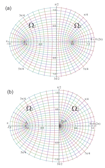
Figure 1: (a)Two-elleptic CS with foci $f_{1}=1$, $f_{2}=0.5$. (b) Degenerated case with foci $f_{1}=1$, $f_{2}=0$.

Now we require the continuity and differentiability of the solution at the boundary $\theta=\pi/2$

$$\Phi_{1}(\frac{\pi}{2})=\Phi_{2}(\frac{\pi}{2}),$$

$$\Phi_{1}^{{}^{\prime}}(\frac{\pi}{2})=\Phi_{2}^{{}^{\prime}}(\frac{\pi}{2}),$$ (26)

and compliancy with Bloch’s theorem on the boundary $\theta=-\pi/2$ ($\theta=3\pi/2$):

$$\Phi_{1}(\frac{3\pi}{2})e^{i2\pi K}=\Phi_{2}(-\frac{\pi}{2}),$$

$$\Phi_{1}^{{}^{\prime}}(\frac{3\pi}{2})e^{i2\pi K}=\Phi_{2}^{{}^{\prime}}(-\frac{\pi}{2}).$$ (27)

(Note, that we distinguish characteristic exponent $K$ for two-elliptic CS from $\nu$ for Mathieu’s functions.)

Substituting expressions Eq. 25 in Eqs. 26, 27, we receive 4 Eqs. for unknown $A_{1},B_{1},A_{2},B_{2}$. The coefficients at $A_{1},B_{1},A_{2},B_{2}$ constitute $4\times 4$ matrix $M$:

$$\left[\begin{array}[]{cccc}ce_{\nu}(\frac{\pi}{2},q_{1})&se_{\nu}(\frac{\pi}{2},q_{1})&-ce_{\nu}(\frac{\pi}{2},q_{2})&-se_{\nu}(\frac{\pi}{2},q_{2})\\ \vskip 6.0pt plus 2.0pt minus 2.0pt\cr ce^{\prime}_{\nu}(\frac{\pi}{2},q_{1})&se^{\prime}_{\nu}(\frac{\pi}{2},q_{1})&-ce^{\prime}_{\nu}(\frac{\pi}{2},q_{2})&-se^{\prime}_{\nu}(\frac{\pi}{2},q_{2})\\ \vskip 6.0pt plus 2.0pt minus 2.0pt\cr\beta ce_{\nu}(\frac{3\pi}{2},q_{1})&\beta se_{\nu}(\frac{3\pi}{2},q_{1})&-ce_{\nu}(-\frac{\pi}{2},q_{2})&-se_{\nu}(-\frac{\pi}{2},q_{2})\\ \vskip 6.0pt plus 2.0pt minus 2.0pt\cr\beta ce^{\prime}_{\nu}(\frac{3\pi}{2},q_{1})&\beta se^{\prime}_{\nu}(\frac{3\pi}{2},q_{1})&-ce^{\prime}_{\nu}(-\frac{\pi}{2},q_{2})&-se^{\prime}_{\nu}(-\frac{\pi}{2},q_{2})\end{array}\right].$$ (32)

We use in 32 the notation: $\beta=\exp i2\pi K$. In order to solve the system 26, 27, the determinant of the matrix $M$ must satisfy the equation

$$\det(M)=0.$$ (33)

This is, basically, the equation for eigenvalues $\lambda$ vs., say, $q_{1}$ if the ratio $\alpha=f_{2}/f_{1}$ is fixed. The solution of 33 can be written in the form

$$\cos 2\pi K=\frac{F(\lambda,q_{1},q_{2})}{2\det(W[q_{1}])\det(W[q_{2}])}.$$ (34)

where $\det(W[q_{1}]),\det(W[q_{2}])$ are Wronskians for fundamental solutions with $q_{1}$ or $q_{2}$

$$\det(W_{q})=ce^{\prime}_{\nu}(,q)se_{\nu}(,q)-ce_{\nu}(,q)se^{\prime}_{\nu}(,q),$$ (35)

(argument $\theta$ does not matter). The function $F(\lambda,q_{1},q_{2})=F(\lambda,q_{1},q_{1}\alpha^{2})$ is bulky expression from determinant calculations. Instead of $ce_{\nu}(\theta,q)$, $ce^{\prime}_{\nu}(\theta,q)$, $se_{\nu}(\theta,q)$, $se^{\prime}_{\nu}(\theta,q)$ we introduce the short notations: $c_{\theta,q},c^{\prime}_{\theta,q},s_{\theta,q},s^{\prime}_{\theta,q}$ with indices $(q_{1},q_{2})=(1,2)$, $(\frac{\pi}{2},-\frac{\pi}{2},\frac{3\pi}{2})=(1,2,3)$. After that, the expression $F(\lambda,q_{1},q_{1}\alpha^{2})$ can be written down in the compact form:

$$F(\lambda,q_{1},q_{1}\alpha^{2})=$$

$$c_{31}c^{\prime}_{12}s_{12}s^{\prime}_{11}+c_{11}c^{\prime}_{12}s_{12}s^{\prime}_{31}-2c_{31}c^{\prime}_{12}s_{11}s^{\prime}_{12}+$$

$$2c_{11}c^{\prime}_{12}s_{31}s^{\prime}_{12}+c_{31}c_{12}s^{\prime}_{11}s^{\prime}_{12}+c_{11}c_{12}s^{\prime}_{31}s^{\prime}_{12}-$$

$$c^{\prime}_{31}(c^{\prime}_{12}s_{11}s_{12}+c_{12}(-2s_{12}s^{\prime}_{11}+s_{11}s^{\prime}_{12}))-$$

$$c^{\prime}_{11}(c^{\prime}_{12}s_{31}s_{12}+c_{12}(2s_{12}s^{\prime}_{31}+s_{31}s^{\prime}_{12})).$$ (36)

The right side of Eq. 34 can not be out of the range $(-1,1)$ of the left side 34, and two conditions:

$$\frac{F(\lambda,q_{1},q_{1}\alpha^{2})}{2\det(W[q_{1}])\det(W[q_{1}\alpha^{2}])}=1,$$ (37)

$$\frac{F(\lambda,q_{1},q_{1}\alpha^{2})}{2\det(W[q_{1}])\det(W[q_{1}\alpha^{2}])}=-1,$$ (38)

define the eigenvalues vs. parameter $q_{1}$ (characteristic curves) for periodic solutions of the system 21, 23. These curves separate the stable solutions from unstable and on these curves the characteristic exponent must be an integer number.

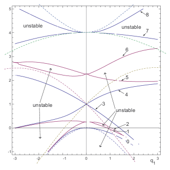
Figure 2: Stability chart for two-elliptic CS with $\alpha^{2}=0.25$ shows the first nine characteristic lines with integer characteristic exponent. The dashed lines show the characteristic lines calculated with Eq.33 for $\alpha^{2}=1$ (E.L.Ince chart for Mathieu’s characteristic values Mclachlan:1947 ).

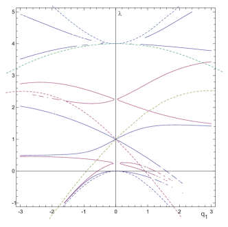
Figure 3: Stability chart for two-elliptic CS with $\alpha^{2}=0.0625$. The dashed lines is Mathieu’s characteristics.

III. Eigenvalues.To find the characteristic curves, we need to solve transcendental equations 37,38. It was done numerically and Fig.2 presents the calculation of characteristic curves for scale coefficient $\alpha=0.5$. Fig.2 demonstrates that all characteristic lines undergo the transformation and in the old regions of stability there are several new ’peninsulas’ of instability. The charts show some discontinuities when $q_{1}$ rises. This artifact is result of lack of accuracy during the solving the transcendental equations 37-38. The real characteristic curve does not have any discontinuity.

There is interesting feature of charts. All of them, except the Mathieu’s, have an additional characteristic values $0.25,2.25,6.25,12.25,...$ at $q_{1}=0$ together with standard characteristic values $0,1,4,9,...$. These characteristic values $0.25,...$ generated by $(n+1/2)^{2}$, $n=0,1,2,...$ were discovered by Meissner Meissner:1918 and B. van der Pol, Strutt PolStrutt:1928 . As seen from whole picture of characteristics, they are related to a discontinuity of the metric (or potential in Eq.21, 23) at $\theta=\pi/2$, which disappears only when $\alpha=1$.

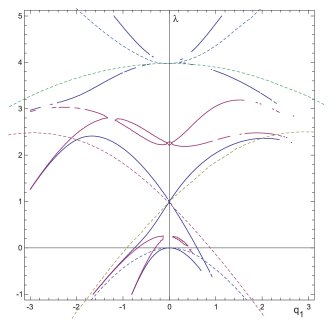
Figure 4: Stability chart for two-elliptic CS with $\alpha^{2}=2.0$. The dashed lines is Mathieu’s characteristics.

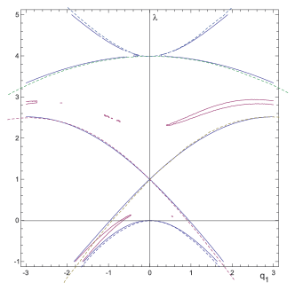
Figure 5: Stability chart for almost symmetric two-elliptic CS with $\alpha^{2}=0.90625$. Interrupted lines are artifacts and the result of a failure in of calculation algorithm. The dashed lines is Mathieu’s characteristics.

However, a different ratio $\alpha$ gives a different chart of characteristic curves, Fig.3-5. The Fig.4 was build for parameter $\alpha>1$. When parameter $\alpha$ is almost near the unity, Fig.5, the chart still contains the new characteristic lines up to limiting point $\alpha=1$.

Because the parameter $\alpha$ can be varied from $0$ to $\infty$, we have an infinite number different stability charts. This gives us infinite number of new orthogonal families of coordinate systems which support the separation of variables.

IV. Eigenfunctions. In order to find the correct eigenfunctions, we need

• select the particular chart by parameter $\alpha$; for example, the parameter $\alpha=0$ gives the family of two-elliptic systems with degenerated right-side (semi-circles on the right side, Fig.1(b) shows only one such CS);

• the choice of the value $q_{1}$ gives a particular coordinate system from the family; the geometry of the potential or specific boundary shape defines this choice.

• ’insert’ the characteristic number (eigenvalue) $\lambda$ taken from intersection of $q_{1}$ and characteristic curves marked by characteristic exponent: $(n=0,1,2...)$ or $(n=1/2,3/2,5/2,...)$ into the general solutions 25. The solution 25 must be stitched on the boundaries by proper 3 coefficients from $A_{1},B_{1},A_{2},B_{2}$.

• normalize each eigenfunction using the free coefficient.

If these can be done for all characteristic exponents, we will receive the set of eigenfunctions

$$ce_{n}(\theta,q_{1},\alpha),\;\;se_{n}(\theta,q_{1},\alpha)$$ (39)

which should be complete and normalized.

There are another alternative ways to build the set of eigenfunctions and eigenvalues for two-elliptic CS, but described is straightforward.

V. Conclusion. There are very few problems for which the SE and HE can be solved exactly. This is mainly due to fact that only high symmetrical boundaries and potentials allow the implementation of the powerful method of the separation of variables. Here, we suggested the two-elliptic CS which is less symmetrical than elliptic, can admit the separation of variables in HE and SE, and includes an infinite number of other families of CS with the same properties. In classical dynamics, thus CS can probably unify the dispersive and regular behavior of particles.

References

(1)
Morse, P. M., and Feshbach, E.L., Methods of Theoretical Physics, vol. 1-2, McGraw-Hill Book Co., New York, 1953.
(2)
W. Miller, Jr. Symmetry and separation of variable, Addison
Wesley, (1977).
(3)
Kovalev, G.V., Polyelliptic coordinates for solving the Schrödinger and Helmholtz
equations (submitted for publication in JETP Letters).
(4)
Bunimovich L.A.: On the ergodic properties of certain billiards. Funct. Anal.
Appi. 8, 254, (1974).
(5)
McLachlan, N.W.: Theory and application of Mathieu functions.
Oxford University Press, (1947).