Appearance of flat surface bands in three-dimensional topological insulators in a ferromagnetic exchange field

Abstract

We study the properties of the surface states in three-dimensional topological insulators in the presence of a ferromagnetic exchange field. We demonstrate that for layered materials like Bi₂Se₃ the surface states on the top surface behave qualitatively different than the surface states at the side surfaces. We show that the group velocity of the surface states can be tuned by the direction and strength of the exchange field. If the exchange field becomes larger than the bulk gap of the material, a phase transition into a topologically nontrivial semimetallic state occurs. In particular, the material becomes a Weyl semimetal, if the exchange field possesses a non-zero component perpendicular to the layers. Associated with the Weyl semimetallic state we show that Fermi arcs appear at the surface. Under certain circumstances either one-dimensional or even two-dimensional surface flat bands can appear. We show that the appearence of these flat bands is related to chiral symmetries of the system and can be understood in terms of topological winding numbers. In contrast to previous systems that have been suggested to possess surface flat bands, the present system has a much larger energy scale, allowing the observation of surface flat bands at room temperature. The flat bands are tunable in the sense that they can be turned on or off by rotation of the ferromagnetic exchange field. Our findings are supported by both numerical results on a finite system as well as approximate analytical results.

1 Introduction

A topological insulator is a material with an insulating energy gap in its bulk, but possesses conducting surface states due to significant spin-orbit coupling. The existence of these surface states is guaranteed by a topological invariant making them particularly robust against time-reversal invariant perturbations or disorder. Due to spin-orbit coupling the surface states are spin-momentum coupled allowing for interesting potential spintronics applications. The dispersion of the surface states forms a Dirac cone, i.e. the conduction electrons at the surface are effectively massless. This peculiar state of matter has first been suggested theoretically [1, 2] and afterwards confirmed experimentally [3, 4, 5, 6, 7, 8]. The number of materials identified as three dimensional topological insulators (3DTI) is steadily increasing [5, 6, 7, 8, 9, 10, 11, 12].

In the present work we study 3DTI in the presence of a ferromagnetic exchange field. Experimentally, it has been demonstrated that such fields can be introduced into topological insulators either by doping with ferromagnetic dopants [15, 16, 17] or by proximity to ferromagnetic materials [18]. As the ferromagnetic exchange field breaks time-reversal symmetry, it allows for controlled modification or removal of the surface states and could lead to interesting effects or devices [13, 14, 15, 19]. In previous work it has been pointed out that depending on the relative orientation of the exchange field with respect to the surface of the topological insulator, the surface states may open an energy gap or remain intact [20, 21, 22, 23]. However, only small exchange splittings have been considered. In the present work we are considering exchange splittings up to the order of the gap of the topological insulator, which is up to 0.3 eV for present materials. Exchange splittings of the order of 1 eV can be reached with ferromagnetic materials.

In a recent work we have studied a two dimensional thin strip of a particle-hole symmetric topological insulator and found that under exchange fields of such strength an edge state flat band can appear [24]. Such flat bands are of particular interest, because the group velocity vanishes allowing highly localized wave packets. Flat bands have been found previously in other condensed matter systems like graphene, superfluid ³He, or unconventional superconductors [25, 26, 27, 28, 29, 30, 31, 32, 33, 34, 35, 36, 37]. In particular, the appearence of flat bands in $d$-wave superconductors as surface Andreev bound states has been studied well in the past both theoretically and experimentally [33, 34, 35, 38, 39, 40, 41, 42, 43, 44, 45]. Such surface flat bands have been shown to lead to an enhanced barrier for vortex entry [46, 47] or increased nonlinear electromagnetic reponse [48, 49, 50]. However, it remained an open question whether flat bands may also appear in three dimensional topological insulators under sufficiently strong ferromagnetic exchange fields.

In the present work, we will present a systematic investigation of the possible surface states of 3DTI and their behavior under a ferromagnetic exchange field. We will show under which circumstances surface flat bands appear. In particular, we identify a case in which a two dimensional flat band can be generated. We demonstrate that the appearence of our flat bands can be understood in terms of a classification recently proposed by Matsuura et al [51] using a topological invariant in the presence of a chiral symmetry. We will also show that the exchange field can produce highly anisotropic Dirac cones, i.e. that the group velocity is different in different directions. In this case the velocity can be tuned by rotation of the exchange field, i.e. rotation of the remanent magnetization of the ferromagnetism.

Recently the possibility of realizing a Weyl semimetallic state in pyrochlore iridates has raised a lot of interest [52]. This state is a generalization of the two-dimensional Dirac electrons in graphene to a three-dimensional bulk system. In a Weyl semimetal conduction band and valence band touch each other only at a finite number of points. These so-called Weyl nodes are exceptionally stable for topological reasons. Of particular interest are the surface states of a Weyl semimetal which may form open Fermi “arcs” [52, 53, 54]. In the present work we show that a 3DTI with a sufficiently strong ferromagnetic exchange field becomes a Weyl semimetal in most cases. The surface flat bands are directly related to the appearence of surface Fermi arcs in this system.

In contrast to previous proposals for surface flat bands in other systems like graphene, superfluid ³He, or unconventional superconductors the present system has the advantage that the relevant energy scale is much larger ($\sim$ 0.3 eV). This allows observation of the flat bands at room temperature, while for all other previous proposals cryogenic temperatures are necessary. In addition, the surface states can be tuned by rotation of the exchange field. For example, the flat band can be turned on and off by a rotation of the remanent magnetization of a ferromagnet. We demonstrate that such behavior can be achieved for realistic material parameters leading to new possible spintronic devices.

2 Models

As a starting point we consider the generic effective two-orbital Hamiltonian for a three dimensional topological insulator suggested already in several previous works [56, 57, 55, 58]. To facilitate numerical calculations we choose the lattice regularized version that has been suggested by Li et al [55]:

$$H(\mathbf{k})=\epsilon_{0}(\mathbf{k})\mathbb{I}_{4\times 4}+\sum_{i=0}^{3}m_{i}(\mathbf{k})\Gamma^{i}+\sum_{\alpha\in\{x,y,z\}}V_{\alpha}\Gamma_{\alpha}$$ (1)

Here, $\epsilon_{0}(\mathbf{k})=C+2D_{2}(1-\cos k_{x})+2D_{2}(1-\cos k_{y})+2D_{1}(1-\cos k_{z})$, $m_{0}(\mathbf{k})=M-2B_{2}(1-\cos k_{x})-2B_{2}(1-\cos k_{y})-2B_{1}(1-\cos k_{z})$, $m_{1}(\mathbf{k})=2A_{2}\sin k_{x}$, $m_{2}(\mathbf{k})=2A_{2}\sin k_{y}$, and $m_{3}(\mathbf{k})=2A_{1}\sin k_{z}$. The Dirac $\Gamma$ matrices are represented by $\Gamma^{0,1,2}=(\mathbb{I}_{2\times 2}\otimes\tau_{x},\sigma_{x}\otimes\tau_{z},\sigma_{y}\otimes\tau_{z})$ in the spin-orbit basis. Here, the Pauli matrices in orbital space are denoted by $\tau_{i}$ and the ones in spin space by $\sigma_{i}$. As has been pointed out by Hao and Lee [59], there exist the following two different choices for $\Gamma^{3}$: $\Gamma^{3}_{I}=\mathbb{I}_{2\times 2}\otimes\tau_{y}$ and $\Gamma^{3}_{II}=\sigma_{z}\otimes\tau_{z}$. These correspond to two different types of spin-orbit coupling in $z$-direction. We follow the convention of Hao and Lee and denote these two choices as model I and model II, respectively. Note that if $k_{z}=0$ there is no difference between the two models. Model I is isotropic within the $xy$-plane, but the coupling in $z$-direction is different. Thus one has qualitatively different behavior of surface states at a $z$-boundary than at an $x$- or $y$-boundary. For model II the spin-orbit coupling is isotropic and it is sufficient to consider surface states at one selected boundary, because the qualitative behavior is the same in all three spatial directions. It has been discussed in Ref. [57] that in the absence of an exchange field model I and model II are related by a unitary transformation and a 90 degree rotation within the $xy$-plane. However, this is not true anymore in the presence of an exchange field, because the spin operators are mapped to pseudospin operators under the unitary transformation as has been pointed out in Ref. [60]. Thus, for the purpose of the present work the two models become different in the presence of an exchange field. Model I is appropriate for Bi₂Se₃ and its relatives.

The components of the ferromagnetic exchange field in $x$, $y$, and $z$-direction are denoted by $V_{x,y,z}$, respectively, and are modeled by Zeeman terms in the Hamiltonian Eq. (1). The matrices for the exchange field components are given by $\Gamma_{\alpha}=\sigma_{\alpha}\otimes\mathbb{I}_{2\times 2}$. The parameters $A_{1}$, $A_{2}$, $B_{1}$, $B_{2}$, $C$, $D_{1}$, $D_{2}$, and $M$ have been derived from bandstructure calculations for the Bi₂Se₃ family of materials in Refs. [56, 57]. In our numerical calculations we will consider the case $A_{i}\geq M>0$ and $B_{i}\geq M$ as is relevant for these materials.

3 Symmetry considerations

Let us first discuss certain symmetries of the Hamiltonian (1) that will be of particular importance in this work. To begin with we focus on the particle-hole symmetric case $C=D_{1}=D_{2}=0$, in which the effects become particularly clear and the topological invariant proposed by Matsuura et al [51] can be used. In Section 7 we will discuss the modifications that appear when particle-hole symmetry is slightly broken, as is the case in the Bi₂Se₃ family of materials.

For $C=D_{1}=D_{2}=0$ the four bulk bands for model I can be found by analytical diagonalization of the $4\times 4$ matrices and are given by

$$E_{i}^{I}(\mathbf{k})=\pm\sqrt{m^{2}+V^{2}\pm 2\sqrt{\left(m_{0}^{2}+m_{3}^{2}\right)V^{2}+\left(m_{1}V_{x}+m_{2}V_{y}\right)^{2}}}$$ (2)

while for model II we have

$$E_{i}^{II}(\mathbf{k})=\pm\sqrt{m^{2}+V^{2}\pm 2\sqrt{m_{0}^{2}V^{2}+\left(m_{1}V_{x}+m_{2}V_{y}+m_{3}V_{z}\right)^{2}}}$$ (3)

where $V^{2}=V_{x}^{2}+V_{y}^{2}+V_{z}^{2}$ and $m^{2}=m_{0}^{2}+m_{1}^{2}+m_{2}^{2}+m_{3}^{2}$. As is clear from these expressions, the bulk spectrum is fully symmetric around energy $E=0$ for both models.

The $\Gamma$ matrices introduced in the previous section respect the following commutation and anti-commutation relations

$$\{\Gamma^{i},\Gamma^{j}\}=2\delta_{ij},$$ (4)

$$[\Gamma_{x},\Gamma^{0}]=[\Gamma_{x},\Gamma_{I}^{3}]=\{\Gamma_{x},\Gamma_{II}^{3}\}=[\Gamma_{x},\Gamma^{1}]=\{\Gamma_{x},\Gamma^{2}\}=0,$$ (5)

$$[\Gamma_{y},\Gamma^{0}]=[\Gamma_{y},\Gamma_{I}^{3}]=\{\Gamma_{y},\Gamma_{II}^{3}\}=[\Gamma_{y},\Gamma^{2}]=\{\Gamma_{y},\Gamma^{1}\}=0,$$ (6)

$$[\Gamma_{z},\Gamma^{0}]=[\Gamma_{z},\Gamma_{I}^{3}]=[\Gamma_{z},\Gamma_{II}^{3}]=\{\Gamma_{z},\Gamma^{1}\}=\{\Gamma_{z},\Gamma^{2}\}=0,$$ (7)

where $\delta_{ij}$ is Kronecker’s delta symbol.

In the absence of an exchange field time reversal symmetry is respected. However, application of an exchange field in any direction breaks time reversal symmetry. According to the classification by Schnyder et al [61, 62] a system with broken time reversal symmetry may still be topologically nontrivial, if a chiral symmetry is present. Let $\Theta$ be a chiral symmetry operator, which by definition anticommutes with the Hamiltonian, i.e.

$$\left\{H(\mathbf{k}),\Theta\right\}=0$$ (8)

If such a symmetry exists, the system falls into the AIII chiral symmetry class [61, 62, 63].

Let us consider the symmetry operator $\Theta_{1}=\sigma_{x}\otimes\tau_{z}$, which happens to be identical to the operator $\Gamma^{1}$. $\Theta_{1}$ anticommutes with $\Gamma^{0}$, $\Gamma^{2}$, $\Gamma_{I}^{3}$, $\Gamma_{II}^{3}$, $\Gamma_{y}$, and $\Gamma_{z}$, but commutes with $\Gamma^{1}$ and $\Gamma_{x}$. Thus, for $k_{x}=0$ and an exchange field within the $y$-$z$-plane Hamiltonian (1) with $C=D_{1}=D_{2}=0$ possesses the chiral symmetry $\Theta_{1}$.

Similarly, we can consider the symmetry operator $\Theta_{2}=\sigma_{y}\otimes\tau_{z}=\Gamma^{2}$. $\Theta_{2}$ anticommutes with $\Gamma^{0}$, $\Gamma^{1}$, $\Gamma_{I}^{3}$, $\Gamma_{II}^{3}$, $\Gamma_{x}$, and $\Gamma_{z}$, but commutes with $\Gamma^{2}$ and $\Gamma_{y}$. Thus, for $k_{y}=0$ and an exchange field within the $x$-$z$-plane Hamiltonian (1) with $C=D_{1}=D_{2}=0$ possesses the chiral symmetry $\Theta_{2}$.

Alternatively, we may also consider the symmetry operator $\Theta_{3}=\sigma_{z}\otimes\tau_{z}$, which happens to be identical to the operator $\Gamma_{II}^{3}$. $\Theta_{3}$ anticommutes with $\Gamma^{0}$, $\Gamma^{1}$, $\Gamma^{2}$, $\Gamma_{I}^{3}$, $\Gamma_{x}$, and $\Gamma_{y}$, but commutes with $\Gamma_{II}^{3}$ and $\Gamma_{z}$. Thus, for model I with exchange field within the $x$-$y$-plane Hamiltonian (1) with $C=D_{1}=D_{2}=0$ possesses the chiral symmetry $\Theta_{3}$. For model II this symmetry is respected for $k_{z}=0$.

From these considerations we see that Hamiltonian (1) under certain circumstances falls into the AIII chiral symmetry class and we have identified three important symmetries.

4 Nonequivalent surface boundaries

Our aim is to calculate the energy dispersion of the surface states for both models, for all possible nonequivalent surfaces perpendicular to $x$-, $y$-, and $z$-directions, and for the corresponding directions of the exchange field. In this way we will determine all possible types of surface states that can appear in a 3DTI in a ferromagnetic exchange field.

For all cases we will present numerical calculations based on an exact diagonalization of Hamiltonian (1) on a finite size lattice of dimension $500\times 500\times 200$. Periodical boundary conditions are employed parallel to the surface with 500 $k$-modes in both directions, while open boundary conditions are used perpendicular to the surface on 200 real space points. Our numerical results are compared with approximate analytical results for a continuous half space using a small $k$ expansion of Hamiltonian (1) near the $\Gamma$ point $\mathbf{k}=0$. For the appearance of the flat bands we will check our results using the topological winding number proposed by Matsuura et al [51].

In total we find that we need to consider seven nonequivalent cases: for model II the spin-orbit coupling in $z$-direction is of the same type as in $x$- and $y$-direction. For that reason it is sufficient to study a single boundary direction, which we choose to be a $y$-boundary, i.e. a boundary with $y=$ const. As regards the direction of the exchange field we have to distinguish two nonequivalent cases here: parallel and perpendicular to the surface, i.e. $V_{x}\neq 0$ and $V_{y}\neq 0$. In contrast, for model I we have five nonequivalent cases. For model I the spin-orbit coupling in $z$-direction is of a different type than in $x$- and $y$-direction, but the in-plane coupling is still isotropic. Therefore we need to distinguish a $z$-boundary and a $y$-boundary. For the $z$-boundary there are again two nonequivalent directions for the exchange field: $V_{x}\neq 0$ and $V_{z}\neq 0$. For the $y$-boundary, however, all field directions are nonequivalent and we have three cases here.

We will see that among these seven cases there are three in which flat surface bands appear. One dimensional flat bands are found for model II with $y$-boundary and exchange field in $x$-direction as well as for model I with $y$-boundary and exchange field in $z$-direction. A two dimensional flat band is found for model I with $y$-boundary and exchange field in $x$-direction.

5 Model I

In this section we discuss the five nonequivalent cases for the particle-hole symmetric model I. We start with the more interesting case of a $y$-boundary.

5.1 Boundary perpendicular to the $y$-direction with finite $V_{y}$

In this case with $V_{x}=V_{z}=0$ the bulk energy bands Eq. (2) simplify to the following expression:

$$E_{i}^{I}(\mathbf{k})=\pm\sqrt{m_{1}^{2}+\left(V_{y}\pm\sqrt{m_{0}^{2}+m_{2}^{2}+m_{3}^{2}}\right)^{2}}$$ (9)

In the absence of an exchange field this band structure usually possesses a gap, because $m_{0}$, $m_{1}$, $m_{2}$, and $m_{3}$ do not become zero simultaneously. Thus, the system is insulating. However, the gap closes when $V_{y}$ reaches a critical value $V_{cr}$, which is derived in appendix I and is of the order of $M$. The Fermi surface at zero energy is then defined by the two equations $m_{1}=0$ and $V_{y}^{2}=m_{0}^{2}+m_{2}^{2}+m_{3}^{2}$. These two equations define a line in three dimensional $(k_{x},k_{y},k_{z})$ space. Therefore the Fermi surface is one-dimensional and the system has entered a semimetallic state. If one looks at the $\Gamma$ point $k_{x}=k_{y}=k_{z}=0$, where $m_{1}=m_{2}=m_{3}=0$ and $m_{0}=M$ it is clear that the semimetallic state is entered at $V_{y}=M$ or closely below. Thus, the parameter $M>0$ sets the scale for the exchange field, at least for the range of the parameters $A_{i}$ and $B_{i}$ considered here. In appendix I we derive the ranges of the exchange field under which the system becomes semimetallic.

To find approximate analytical solutions for the surface states we expand Hamiltonian (1) up to second order in $k_{y}$. If we assume a boundary in $y$-direction the momentum $k_{y}$ has to be replaced by the momentum operator $-i\partial_{y}$. To find the surface states we search for nontrivial solutions of the Schrödinger equation that vanish both at $y=0$ and for $y\rightarrow\infty$. In this case the Hamiltonian can be written as

$$H(\bf k) =H_{0}(\mathbf{k})+H^{\prime}(\mathbf{k}),$$ (10)

where

$$H_{0}(\mathbf{k}) =(\tilde{m}_{0}(\mathbf{k})+B_{2}\partial_{y}^{2})\Gamma^{0}-i2A_{2}\partial_{y}\Gamma^{2},$$ (11)

$$H^{\prime}(\mathbf{k}) =m_{1}(\mathbf{k})\Gamma^{1}+m_{3}(\mathbf{k})\Gamma_{I}^{3}+V_{y}\Gamma_{y}.$$ (12)

Here, $\tilde{m}_{0}(\mathbf{k})=M-2B_{2}(1-\cos k_{x})-2B_{1}(1-\cos k_{z})$ and $\mathbf{k}=(k_{x},k_{z})$. $\Gamma_{I}^{3}$ anticommutes with $H_{0}$. $\Gamma_{y}$ commutes with both $H_{0}$ and $\Gamma_{I}^{3}$, and $\Gamma^{1}$ anticommmutes with $H_{0}$, $\Gamma_{I}^{3}$, and $\Gamma_{y}$. In this case the eigenstates of $H({\bf k})$ are linear combinations of (up to four) eigenstates of $H_{0}({\bf k})$ (see appendix II for a more detailed explanation). Surface states of $H$ are superpositions of surface states of $H_{0}$. Following the general procedure from appendix II we will first determine the surface states of $H_{0}$ and then deduce the ones of $H$ from them.

For a system of finite width in $y$-direction, the energy of the surface states of $H_{0}$ behaves like $e^{-L}$ as a function of the system size $L$ in the $y$-direction. Let us consider a half infinite system with a single boundary at $y=0$. In this case the surface states of $H_{0}$ have zero energy. To find these zero energy eigenstates we can exploit that $H_{0}$ commutes with the operator $\Theta_{4}=\sigma_{x}\otimes\tau_{x}$. Then there exist simultaneous eigenstates of $H_{0}$ and $\Theta_{4}$. The eigenstates of $\Theta_{4}$ are $(1,0,0,1)^{T}$ and $(0,1,1,0)^{T}$ with eigenvalue $+1$ and $(1,0,0,-1)^{T}$ and $(0,1,-1,0)^{T}$ with eigenvalue $-1$. We try the following two ansätze:

$$\psi_{1,\mathbf{k}}(y)=C(1,0,0,1)^{T}f_{\mathbf{k}}(y),$$ (13)

$$\psi_{2,\mathbf{k}}(y)=C(0,1,-1,0)^{T}f_{\mathbf{k}}(y),$$ (14)

where $C$ is a normalization constant and $f_{\mathbf{k}}(y)$ is solution of the equation

$$[\tilde{m}_{0}(\mathbf{k})+B_{2}\partial_{y}^{2}+2A_{2}\partial_{y}]f_{\mathbf{k}}(y)=0,$$ (15)

The other two eigenstates of $\Theta_{4}$ lead to exponentially increasing functions with $y$ and thus cannot fulfil the boundary condition for $y\rightarrow\infty$. Solving the differential equation (15) we find that $f_{\mathbf{k}}(y)$ is given by

$$f_{\mathbf{k}}(y)=e^{-\frac{A_{2}}{B_{2}}y}\sinh\left(\sqrt{\frac{A_{2}^{2}}{B_{2}^{2}}-\frac{\tilde{m}_{0}(\mathbf{k})}{B_{2}}}\;y\right).$$ (16)

This solution can only fulfil the boundary condition for $y\rightarrow\infty$, if $\tilde{m}_{0}(\mathbf{k})>0$. For those $\mathbf{k}$ values where this condition is not fulfilled anymore, a surface state does not exist.

Having determined the surface states of $H_{0}$ we can now infer the ones of $H$ by noting that $H^{\prime}$ just couples the two solutions Eq. (13) and (14) as

$$\Psi_{\mathbf{k}}(y)=(u_{\mathbf{k}},v_{\mathbf{k}},-v_{\mathbf{k}},u_{\mathbf{k}})^{T}f_{\mathbf{k}}(y).$$ (17)

Here, $u$ and $v$ are the components of the solution spinor $\xi_{\mathbf{k}}=(u_{\mathbf{k}},v_{\mathbf{k}})^{T}$ of the following eigenequation

$$\left[(V_{y}-m_{3}(\mathbf{k}))\sigma_{y}+m_{1}(\mathbf{k})\sigma_{x}\right]\xi_{\mathbf{k}}=E\xi_{\mathbf{k}}.$$ (18)

The full surface state solutions are then given by

$$\Psi_{\pm,\mathbf{k}}(y)=\frac{C}{\sqrt{2}}(1,\pm e^{i\theta_{\mathbf{k}}},\mp e^{i\theta_{\mathbf{k}}},1)^{T}f_{\mathbf{k}}(y),$$ (19)

where

$$\sin\theta_{\mathbf{k}}=\frac{V_{y}-2A_{1}\sin k_{z}}{\sqrt{(V_{y}-2A_{1}\sin k_{z})^{2}+4A_{2}^{2}\sin^{2}k_{x}}},$$

with the corresponding eigenenergies

$$E_{\pm}(\mathbf{k}) =\pm\sqrt{(V_{y}-2A_{1}\sin k_{z})^{2}+4A_{2}^{2}\sin^{2}k_{x}}.$$ (20)

These solutions show that we have surface states as long as $\tilde{m}_{0}(\mathbf{k})>0$. For small momenta the dispersion Eq. (20) shows that the presence of the exchange field in $y$-direction shifts the surface Dirac cone in $k_{z}$-direction. The Dirac cone remains ungapped and its velocity is unchanged.

In Fig. 1 we show results obtained from numerical calculation of the eigenenergies of a finite slab on a finite size lattice for the present case showing nice agreement with the analytical result. Here and in the following we are showing results for the parameter choice $A_{1}=A_{2}=B_{1}=B_{2}=M=1$ and $C=D_{1}=D_{2}=0$. Results for parameters appropriate for Bi₂Se₃ are discussed in section 7. Fig. 1(a) (for $k_{z}=0$) and (c) (for $k_{x}=0$) show the dispersion in the insulating state for a small exchange field of $V_{y}/M=0.2$. In Fig. 1(b) and (d) the semimetallic state with $V_{y}/M=2.0$ is shown. In the present case no surface flat band occurs. Note, that in Fig. 1(c) four surface state dispersions are seen. Only two of them correspond to Eq. (20). The other two dispersions are localized on the opposite surface, which is present in the numerical calculation. These states are related by parity to the ones found analytically above. Their dispersion is thus obtained from Eq. (20) by changing $(k_{x},k_{z})\rightarrow(-k_{x},-k_{z})$, i.e.

$$E_{\pm,2}(\mathbf{k}) =\pm\sqrt{(V_{y}+2A_{1}\sin k_{z})^{2}+4A_{2}^{2}\sin^{2}k_{x}}.$$ (21)

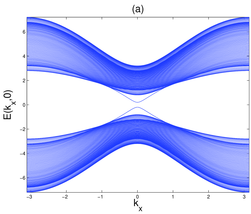
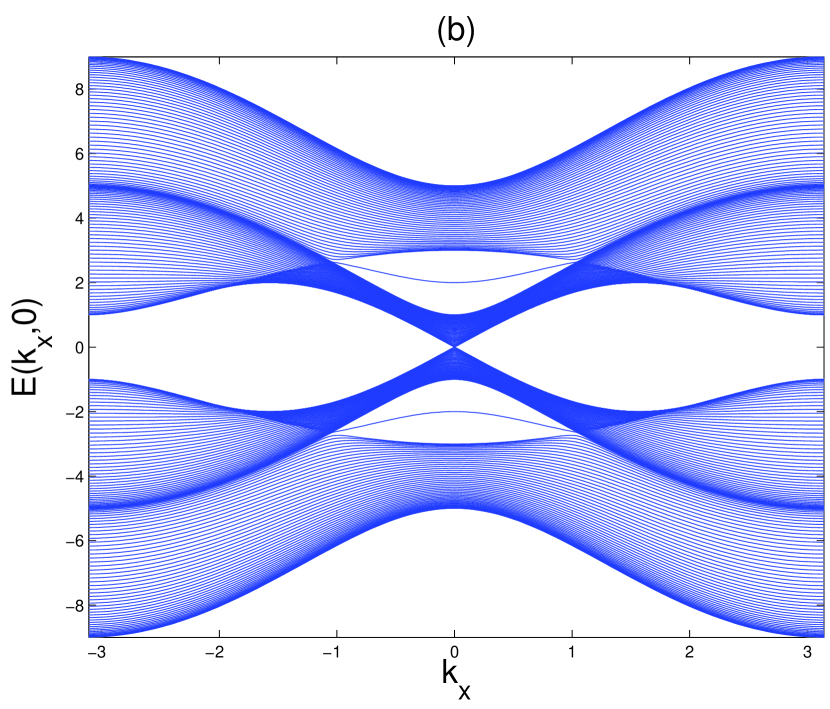
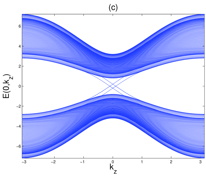
Figure 1: Numerical dispersions of bulk and surface states for model I with $V_{y}/M=0.2$ for (a) and (c) and $2.0$ for (b) and (d). In (a) and (b) $k_{z}=0$, and in (c) and (d) $k_{x}=0$. We have used $B_{1}=B_{2}=A_{1}=A_{2}=M=1$, and $C=D=0$.

We note that the surface states Eq. (19) possess an interesting nontrivial spin texture. To see this we evaluate the expectation value of the spin components in the two orbitals. For orbital 1 the spin matrices can be written in the form

$$\hat{s}_{1,i}=\sigma_{i}\otimes\frac{1}{2}\left(\mathbb{I}_{2\times 2}+\tau_{z}\right)$$ (22)

where $\sigma_{i}$ for $i\in\{x,y,z\}$ are the spin Pauli matrices. For orbital 2 we have analogously

$$\hat{s}_{2,i}=\sigma_{i}\otimes\frac{1}{2}\left(\mathbb{I}_{2\times 2}-\tau_{z}\right)$$ (23)

Using Eq. (19) we find the following expectation values in orbital 1:

$$\left\langle\Psi_{\pm,\mathbf{k}}\left|\hat{s}_{1,x}\right|\Psi_{\pm,\mathbf{k}}\right\rangle =\pm\frac{1}{2}\cos\theta_{\mathbf{k}}$$

$$\left\langle\Psi_{\pm,\mathbf{k}}\left|\hat{s}_{1,y}\right|\Psi_{\pm,\mathbf{k}}\right\rangle =\pm\frac{1}{2}\sin\theta_{\mathbf{k}}$$

$$\left\langle\Psi_{\pm,\mathbf{k}}\left|\hat{s}_{1,z}\right|\Psi_{\pm,\mathbf{k}}\right\rangle =0$$

and in orbital 2:

$$\left\langle\Psi_{\pm,\mathbf{k}}\left|\hat{s}_{2,x}\right|\Psi_{\pm,\mathbf{k}}\right\rangle =\mp\frac{1}{2}\cos\theta_{\mathbf{k}}$$

$$\left\langle\Psi_{\pm,\mathbf{k}}\left|\hat{s}_{2,y}\right|\Psi_{\pm,\mathbf{k}}\right\rangle =\pm\frac{1}{2}\sin\theta_{\mathbf{k}}$$

$$\left\langle\Psi_{\pm,\mathbf{k}}\left|\hat{s}_{2,z}\right|\Psi_{\pm,\mathbf{k}}\right\rangle =0$$

From these expressions we see that the spin rotates within the $x$-$y$ plane. The spin direction of the two surface states is always opposite. The spin-$x$-component is opposite in the two orbitals, while the spin-$y$-component is the same in the two orbitals. Therefore, the total spin points in $y$-direction, perpendicular to the surface:

$$\left\langle\Psi_{\pm,\mathbf{k}}\left|\Gamma_{x}\right|\Psi_{\pm,\mathbf{k}}\right\rangle =0$$

$$\left\langle\Psi_{\pm,\mathbf{k}}\left|\Gamma_{y}\right|\Psi_{\pm,\mathbf{k}}\right\rangle =\pm\sin\theta_{\mathbf{k}}$$

$$\left\langle\Psi_{\pm,\mathbf{k}}\left|\Gamma_{z}\right|\Psi_{\pm,\mathbf{k}}\right\rangle =0$$

Note, that while the total spin is perpendicular to the surface momentum, the partial spins in the two orbitals are not.

5.2 Boundary perpendicular to the $y$-direction with finite $V_{x}$

Let us consider next the case that both $V_{x}$ and $V_{y}$ are nonzero, but still $V_{z}=0$. It is useful to go over to polar coordinates in this case and write $V_{x}=V_{0}\cos\vartheta$ and $V_{y}=V_{0}\sin\vartheta$. The bulk energy bands Eq. (2) can then be brought into the following form:

$$E_{i}^{I}(\mathbf{k}) =\pm\Big{\{}\left(m_{1}\sin\vartheta-m_{2}\cos\vartheta\right)^{2}+$$ (24)

$$+\left(V_{0}\pm\sqrt{m_{0}^{2}+m_{3}^{2}+\left(m_{1}\cos\vartheta+m_{2}\sin\vartheta\right)^{2}}\right)^{2}\Big{\}}^{1/2}$$

Compared with Eq. (9) this corresponds to a rotation of the exchange field within the $x$-$y$-plane. Again, the system is insulating in the absence of an exchange field and the gap closes, when $V_{0}$ reaches the critical value $V_{cr}$. In the semimetallic state the Fermi surface is defined by the two equations $m_{1}\sin\vartheta-m_{2}\cos\vartheta=0$ and $V_{0}^{2}=m_{0}^{2}+m_{3}^{2}+\left(m_{1}\cos\vartheta+m_{2}\sin\vartheta\right)^{2}$. Therefore, the Fermi surface is still one-dimensional.

Determination of the surface states becomes more difficult now, because $\Gamma_{x}$ neither commutes nor anticommutes with $H_{0}$ in Eq. (11). As a result, it affects the spatial part of the surface states. We can, however, determine the surface states of the Hamiltonian

$$H^{\prime}_{0}(\mathbf{k})=H_{0}(\mathbf{k})+V_{x}\Gamma_{x}\,.$$ (25)

$H^{\prime}_{0}(\mathbf{k})$ still commutes with $\Theta_{4}=\sigma_{x}\otimes\tau_{x}$ and we can thus look for zero energy states of $H^{\prime}_{0}(\mathbf{k})$ using the same ansatz Eq. (13) and (14) as before. The surface state solutions of $H^{\prime}_{0}$ (with a boundary at $y=0$ and a half infinite system as before) are then found to be

$$\psi_{1,\mathbf{k}}(y) =C(1,0,0,1)^{T}e^{-\frac{A_{2}}{B_{2}}y}\sinh\left(\sqrt{\frac{A_{2}^{2}}{B_{2}^{2}}-\frac{\tilde{m}_{0}(\mathbf{k})+V_{x}}{B_{2}}}\;y\right),$$ (26)

$$\psi_{2,\mathbf{k}}(y) =C^{\prime}(0,1,-1,0)^{T}e^{-\frac{A_{2}}{B_{2}}y}\sinh\left(\sqrt{\frac{A_{2}^{2}}{B_{2}^{2}}-\frac{\tilde{m}_{0}(\mathbf{k})-V_{x}}{B_{2}}}\;y\right),$$ (27)

where $C$ and $C^{\prime}$ are normalization constants. It is clear that state $1$ exists only if $\tilde{m}_{0}(\mathbf{k})+V_{x}>0$ and state $2$ exists only if $\tilde{m}_{0}(\mathbf{k})-V_{x}>0$.

The matrices $\Gamma^{1}$, $\Gamma_{I}^{3}$, or $\Gamma_{y}$ neither commute nor anticommute with $H^{\prime}_{0}$. Thus they affect the spatial part of the surface states as well as the spin part. In this case we cannot separate the Hamiltonian into parts. However, if $|\mathbf{k}|$ and $V_{y}$ are small we can treat $H^{\prime}$ Eq. (12) as a perturbation using degenerate perturbation theory. We assume that the perturbation only couples the two surface states $1$ and $2$ to each other and neglect coupling to bulk states. This is a reasonable assumption, as the surface states are well localized and in most cases well separated in energy from the bulk states. In this case the overlap between the bulk states and the surface states is very small. Also, due to the symmetric energy spectrum around $E=0$ for each bulk state with energy $E$ there exists another one with energy $-E$. Thus, their contributions tend to cancel each other in perturbation theory.

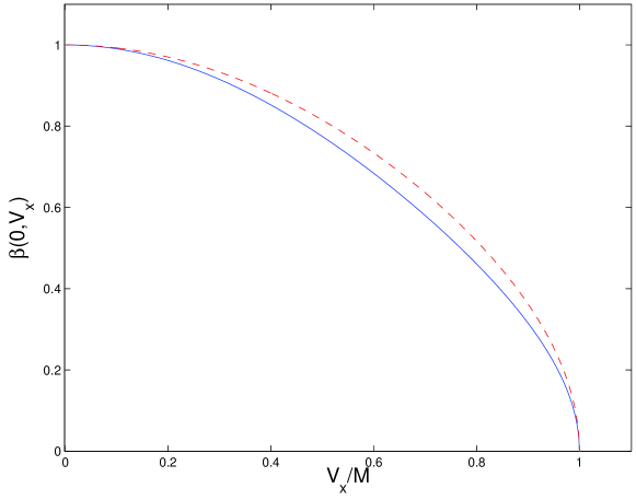
Figure 2: The parameter $\beta$ Eq. (30) as a function of $V_{x}/M$ for two sets of parameters: dashed red line for $A_{1}=A_{2}=B_{1}=B_{2}=M=1$, solid blue line for the Bi₂Se₃ set of parameters in section 7.

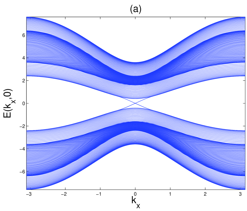
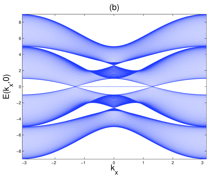
Figure 3: Numerical dispersions of bulk and surface states for model I with $V_{x}/M=0.6$ for (a) and (c) and $2.0$ for (b) and (d). In (a) and (b) $k_{z}=0$, and in (c) and (d) $k_{x}=0$. The other parameters are same as in figure 1.

If both states $1$ and $2$ exist, the surface states for the full Hamiltonian $H$ are then approximately given by

$$\Psi_{\pm,\mathbf{k}}(y) =\frac{1}{\sqrt{2}}(\psi_{1,\mathbf{k}}(y)\pm e^{i\theta_{\mathbf{k}}}\psi_{2,\mathbf{k}}(y)),$$ (28)

where

$$\sin\theta_{\mathbf{k}}=\frac{2A_{1}\sin k_{z}-V_{y}}{\sqrt{(2A_{1}\sin k_{z}-V_{y})^{2}+4A_{2}^{2}\sin^{2}k_{x}}}.$$

The surface state eigenenergies in this case are found to be

$$E_{\pm}(\mathbf{k}) =\pm\beta(V_{x},\mathbf{k})\sqrt{(2A_{1}\sin k_{z}-V_{y})^{2}+4A_{2}^{2}\sin^{2}k_{x}},$$ (29)

where

$$\beta(V_{x},\mathbf{k})= CC^{\prime}\int_{0}^{\infty}\,dy\,\bigg{[}e^{-2\frac{A_{2}}{B_{2}}y}\sinh\left(\sqrt{\frac{A_{2}^{2}}{B_{2}^{2}}-\frac{\tilde{m}_{0}(\mathbf{k})}{B_{2}}+\frac{V_{x}}{B_{2}}}\;y\right)$$ (30)

$$\times\sinh\left(\sqrt{\frac{A_{2}^{2}}{B_{2}^{2}}-\frac{\tilde{m}_{0}(\mathbf{k})}{B_{2}}+\frac{V_{x}}{B_{2}}}\;y\right)\bigg{]}$$

$$=\frac{4A_{2}^{2}\sqrt{{\tilde{m}}^{2}_{0}(\mathbf{k})-V_{x}^{2}}}{4A_{2}^{2}\tilde{m}_{0}(\mathbf{k})+B_{2}V_{x}^{2}}$$

is the spatial overlap of the two states Eq. (26) and (27). The dependence of $\beta$ as a function of $V_{x}$ at $k=0$ is shown in Fig. 2.

For small momenta the dispersion Eq. (29) shows that the presence of an exchange field within the $xy$-plane does not affect the presence of the surface Dirac cone. The Dirac cone is just shifted in $k_{z}$-direction and remains ungapped. However, the velocity of the Dirac cone is isotropically suppressed by the factor $\beta(V_{x},\mathbf{k})$. Thus, the presence of an exchange field component in $x$-direction allows tuning of the group velocity of the surface states, as shown in Fig. 2.

The spin texture of the surface states Eq. (28) turns out to be the same as in the previous section, except for the fact that all spin components are suppressed by the factor $\beta(V_{x},\mathbf{k})$. Thus, the presence of the $x$-component of the exchange field $V_{x}$ leads to a suppression of the spin polarization of the surface states.

Figure 3 shows dispersions with exchange field $(V_{x},0,0)$. One can see from the figure that in this case $k_{x}$- and $k_{z}$-direction are equivalent. This is due to the fact that $\Gamma_{x}$ commutes with both $\Gamma^{1}$ and $\Gamma^{3}$. In Fig. 1 (b) and (d) we see that a flat band appears, if $V_{x}>M$. This flat band is apparently two dimensional, as it stays flat in both $k_{x}$ and $k_{z}$ direction. It still exists if we add a finite $V_{y}$. The existence of this flat band goes beyond the perturbative treatment above. In the next subsection we discuss the existence of this flat band in terms of a topological invariant recently proposed by Matsuura et al.[51]

5.3 Existence of a two-dimensional flat band

Matsuura et al.[51] presented a general classification of the gapless topological phases like in semimetals or nodal superconductors. They showed that a generalized bulk-boundary correspondence exists that relates the topological properties of the Fermi surface to the presence of protected flat bands at the surface of the system. In particular, it was found that the dimension of the surface flat band is always given by the dimension of the Fermi surface plus 1, if it exists (see Table V in Ref.[51]).

In the present case the system is topologically nontrivial and belongs to class AIII as discussed in section 3. The Fermi surface is one-dimensional and we may thus expect the appearance of a two-dimensional flat band.

The presence or absence of the flat band can be classified by a topological winding number. To construct this winding number, we use the chiral symmetry $\Theta_{3}=\sigma_{z}\otimes\tau_{z}$ that was discussed in section 3 and is valid in the present case. Whenever a chiral symmetry is present, the Hamiltonian anticommutes with the symmetry operator. In this case the bulk Hamiltonian can be brought into off-diagonal block form by transforming to the eigenbasis of $\Theta_{3}$:

$$H(\mathbf{k}) =\left(\begin{array}[]{cc}0&D^{\dagger}(\mathbf{k})\\ D(\mathbf{k})&0\end{array}\right),$$ (33)

where the block $D(\mathbf{k})$ is found to be

$$D(\mathbf{k})=\left(\begin{array}[]{cc}m_{0}(\mathbf{k})+im_{3}(\mathbf{k})&-m_{1}(\mathbf{k})+im_{2}(\mathbf{k})+V_{x}-iV_{y}\\ m_{1}(\mathbf{k})+im_{2}(\mathbf{k})+V_{x}+iV_{y}&m_{0}(\mathbf{k})-im_{3}(\mathbf{k})\end{array}\right).$$ (34)

From the block $D(\mathbf{k})$ we can define a winding number [64, 51]

$$w =\frac{1}{2\pi}\textrm{Im}\int\,dk_{\perp}\,\textrm{Tr}\left(D^{-1}(\mathbf{k})\partial_{k_{\perp}}D(\mathbf{k})\right)$$

$$=\frac{1}{2\pi}\textrm{Im}\int\,dk_{\perp}\,\textrm{Tr}\left(\partial_{k_{\perp}}\ln D(\mathbf{k})\right)$$

$$=\frac{1}{2\pi}\textrm{Im}\int\,dk_{\perp}\,\partial_{k_{\perp}}\ln\textrm{det}D(\mathbf{k})$$

$$=\frac{1}{2\pi}\textrm{Im}\int\,dk_{\perp}\,\left(\textrm{det}D(\mathbf{k})\right)^{-1}\partial_{k_{\perp}}\textrm{det}D(\mathbf{k}).$$

Here, $k_{\perp}$ is the momentum component perpendicular to the surface. The winding number $w$ is always an integer and depends on the momentum components parallel to the surface. It measures the phase change of the complex number $\textrm{det}\,D(\mathbf{k})$, when $k_{\perp}$ runs through the Brillouin zone. If $w(k_{||})=0$, there exists no zero energy state for the momentum $k_{||}$ at the surface. If $w(k_{||})$ is nonzero, a zero energy surface state exists. In the present case, where we consider a boundary in $y$-direction we have

$$w(k_{x},k_{z})=\frac{1}{2\pi}\textrm{Im}\int_{-\pi}^{\pi}\,dk_{y}\,\partial_{k_{y}}\ln\textrm{det}D(\mathbf{k}).$$ (36)

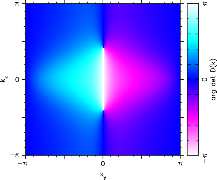
Figure 4: The phase of $\textrm{det}\,D(\mathbf{k})$ for $k_{x}=0$ as a function of $k_{y}$ and $k_{z}$ in a color coded scale. The parameters are the same as in Fig. 3 (b) and (d).

Fig. 4 shows the phase of $\textrm{det}\,D(\mathbf{k})$ for $k_{x}=0$ as a function of $k_{y}$ and $k_{z}$ in a color coded scale for the same set of parameters as in Fig. 3 (b) and (d). Blue color corresponds to phase 0 and white to phase $\pm\pi$. From the figure one notices that there exist a momentum space vortex and an anti-vortex at the positions $(k_{y},k_{z})=(0,\pm 1.318)$, around which the phase winds by $2\pi$. These positions are points on the bulk Fermi surface. Note that $\textrm{det}\,D(\mathbf{k})=0$ on the Fermi surface and the phase becomes singular there. From Fig. 4 it becomes clear that the winding number (36) becomes 1, when $k_{z}\in[-1.318,1.318]$ and 0 outside. This is just the momentum range of the flat band seen in Fig. 3 (b). This example demonstrates that the winding number (36) correctly predicts the presence of the flat band.

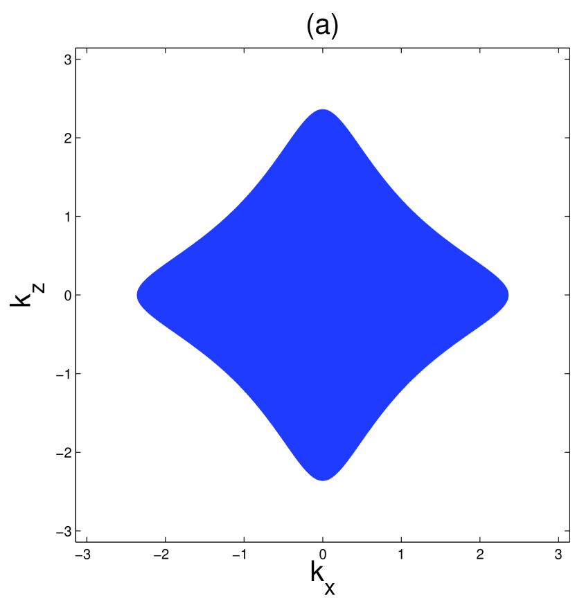
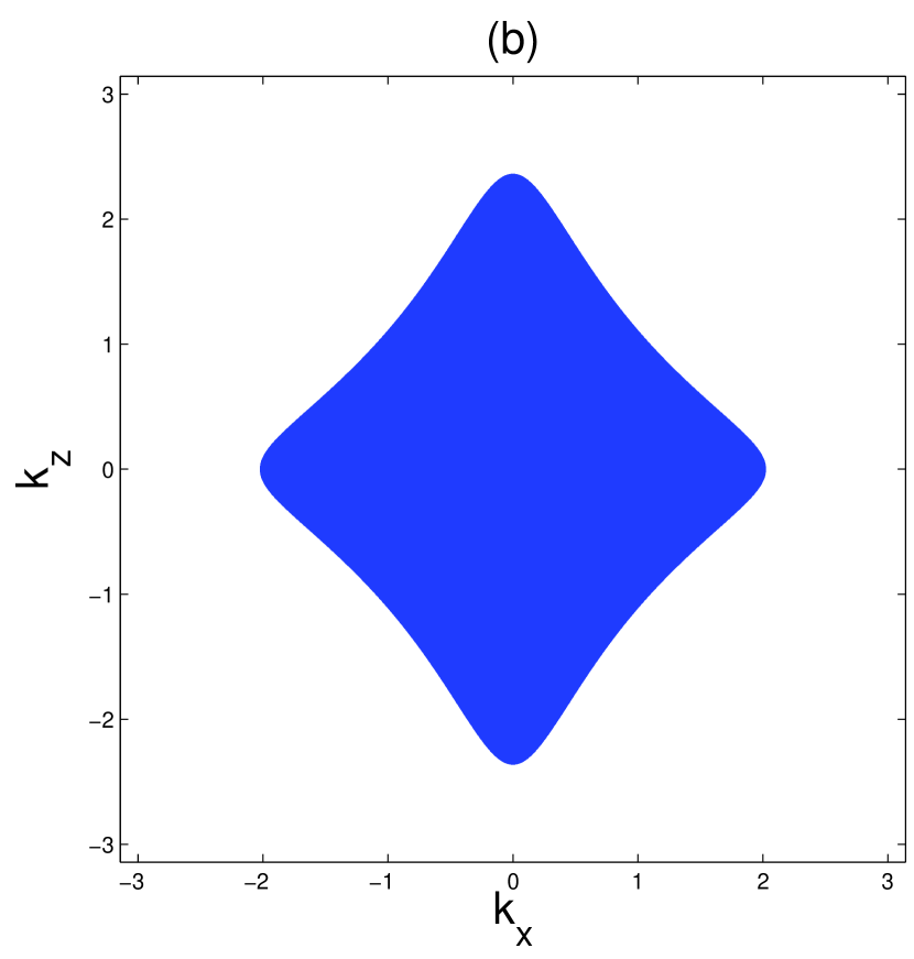
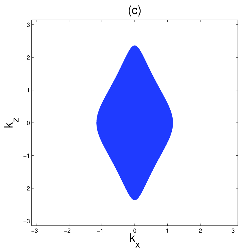
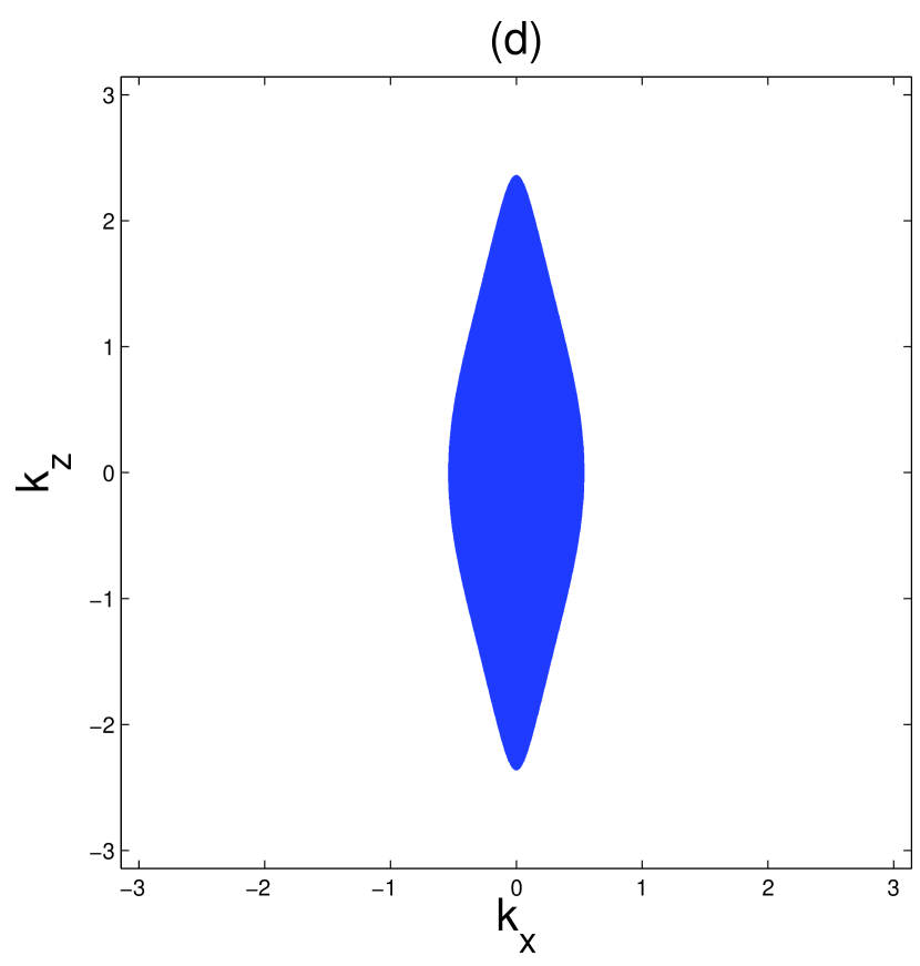
Figure 5: The flat band area within the $(k_{x},k_{z})$-plane for different directions of the exchange field. The field $(V_{x},V_{y})$ is given by $(V_{0},0.0)$ (a), $V_{0}(\cos\pi/8,\sin\pi/8)$ (b), $V_{0}/\sqrt{2}(1,1)$ (c), and $V_{0}(\sin\pi/8,\cos\pi/8)$ (d), respectively. Here, $V_{0}/M=2.8$, $B_{i}=A_{i}=M=1$, and $C=D=0$. The size of the flat band area is reduced when the exchange field is rotated towards the $y$-direction.

Using Eq. (36) we can derive an analytical condition for the existence of the flat band, which is given in appendix III. In Figures 5 and 6 we show the regions in $(k_{x},k_{z})$-space in which the two-dimensional flat band on the $y=0$ surface appears for different sets of parameters. These areas were calculated using the analytical condition from appendix III. Note, that the boundaries of these areas are just the projections of the one-dimensional Fermi surface onto the $(k_{x},k_{z})$-plane, as shown in appendix III.

Figure 5 illustrates the effect of a rotation of the exchange field within the $xy$-plane on the flat band area. The flat band area is shown for exchange fields $V_{x}=V_{0}\cos\vartheta$ and $V_{y}=V_{0}\sin\vartheta$ with $V_{0}=2.8M$ and four angles of rotation $\vartheta$. When the direction of the field is rotated from the $x$-direction into $y$-direction the size of the flat band area is reduced in $x$-direction but remains unchanged in $z$-direction. When the exchange field points in $y$-direction, the flat band finally disappears.

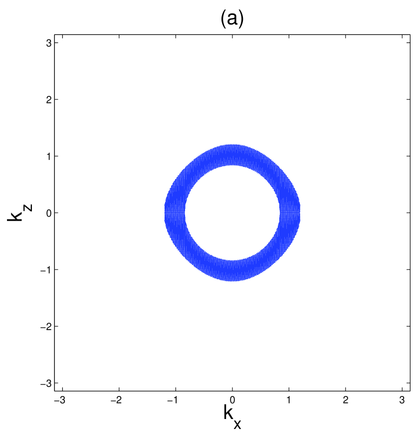
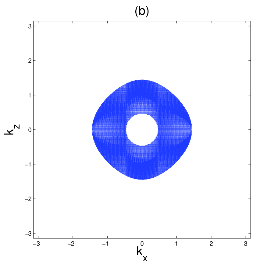
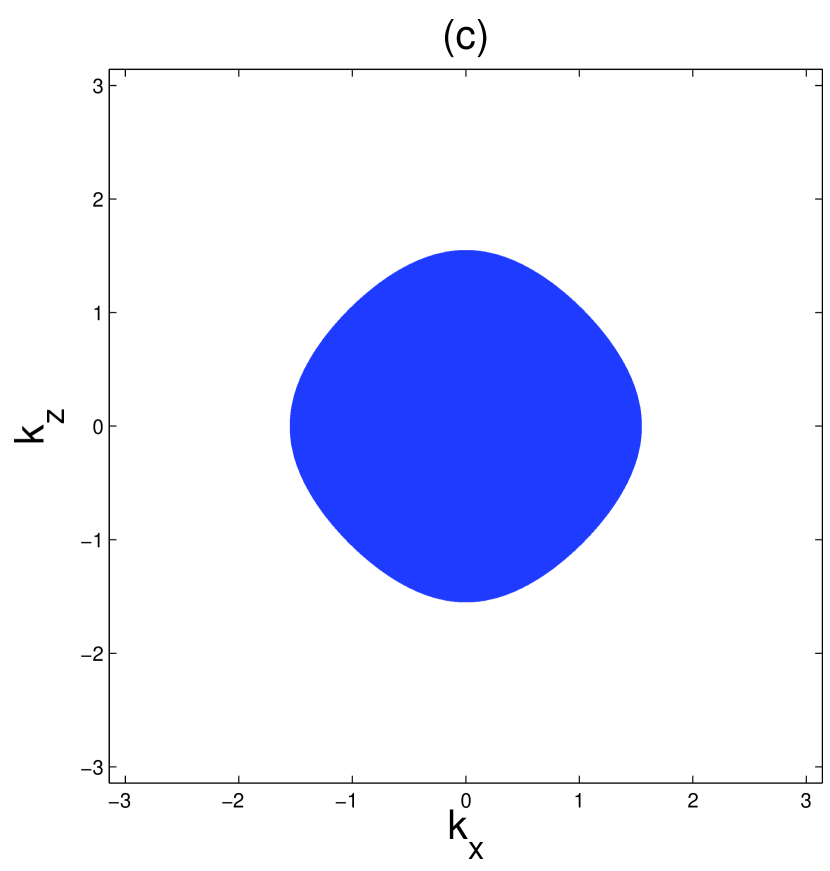
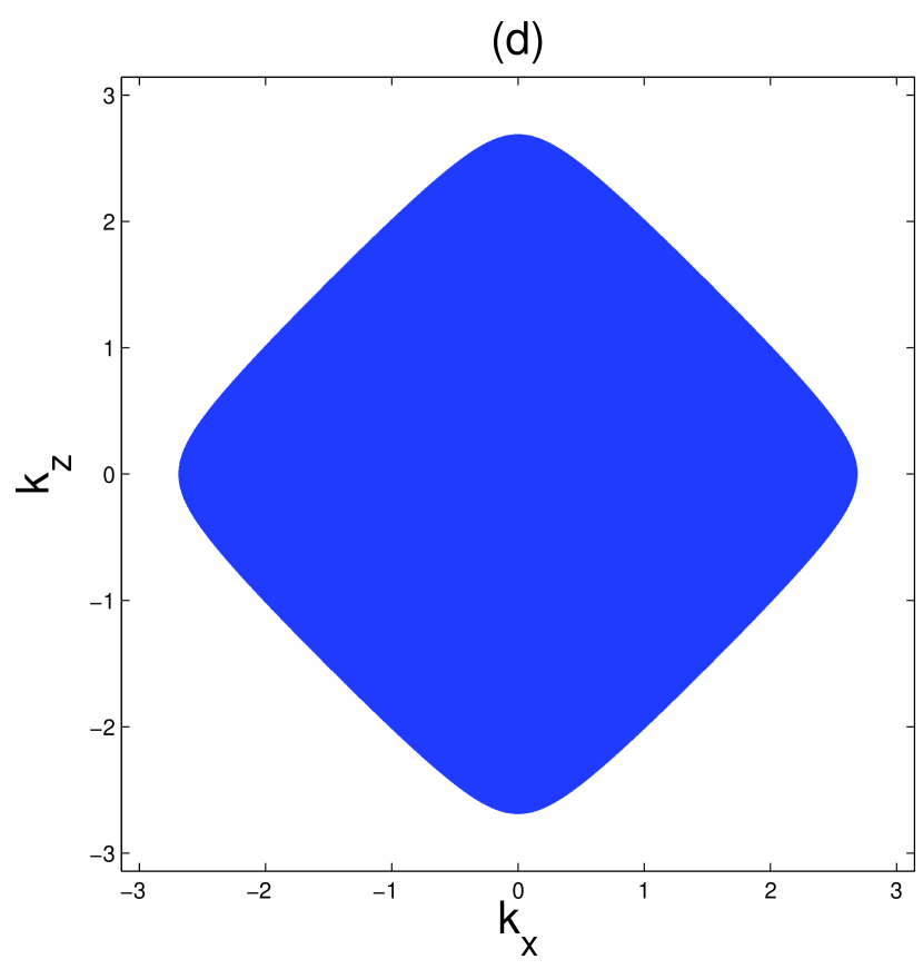
Figure 6: The flat band area within the $(k_{x},k_{z})$-plane for different values of the exchange field in $x$-direction. $V_{x}/M=0.4$ (a) , $V_{x}/M=0.8$ (b), $V_{x}/M=1.0$ (c), and $V_{x}/M=2.8$ (d). Here, we have used the parameters $V_{y}=V_{z}=0$, $B_{i}=M=1$, and $A_{i}=0.15$.

In appendix I we show that for $M<2A_{1}^{2}/B_{1}$ the minimal strength of the exchange field to create a semimetallic state and thus a two-dimensional surface flat band for the present case is given by $V_{cr}=M$. However, if $M>2A_{1}^{2}/B_{1}$ (implicitly assuming $B\geq A$ and $B\geq M$), the minimal exchange field strength is given by the more complicated expression

$$V_{cr}=\frac{A_{1}\sqrt{4B_{1}M-4A_{1}^{2}-M^{2}}}{\sqrt{B_{1}^{2}-A_{1}^{2}}}.$$ (37)

which is smaller than $M$. In this case we can have the situation that the flat band area is not simply connected anymore as shown in figures 6 (a) and (b). This case appears, when Eq. (125) from appendix I possesses two solutions instead of just one.

5.4 Boundary perpendicular to the $y$-direction with finite $V_{z}$

Next, we consider the case that $V_{z}$ is nonzero and $V_{x}=0$. The component $V_{y}$ will be treated perturbatively like in section 5.2. The bulk energy bands Eq. (2) in this case simplify to

$$E_{i}^{I}(\mathbf{k})=\pm\sqrt{m_{1}^{2}+m_{2}^{2}+\left[V_{z}\pm\sqrt{m_{0}^{2}+m_{3}^{2}}\right]^{2}}$$ (38)

Again, the system is insulating in the absence of an exchange field and the gap closes, when $V_{z}$ reaches the critical value $V_{cr}$. In the semimetallic state the Fermi surface is defined now by three instead of two equations, $m_{1}=m_{2}=0$ and $V_{z}^{2}=m_{0}^{2}+m_{3}^{2}$. For this reason, the Fermi surface becomes zero-dimensional, i.e. there are point nodes.

In this case the chiral symmetry $\Theta_{3}$ does not hold anymore, because $\Theta_{3}$ commutes with $\Gamma_{z}$. However, as discussed in section 3 for the special case $k_{x}=0$ the system possesses the chiral symmetry $\Theta_{1}$. For that reason we may expect a one-dimensional flat band with $k_{x}=0$ in this case.

To determine the surface states in second order in $k_{y}$ one first notices that $\Gamma_{z}$ neither commutes nor anticommutes with $H_{0}$. Therefore, it affects the spatial part of the surface states. However, similarly as in section 5.2, we can determine the zero energy surface states of the Hamiltonian

$$H^{\prime\prime}_{0}(\mathbf{k})=H_{0}(\mathbf{k})+V_{z}\Gamma_{z}=(\tilde{m}_{0}(\mathbf{k})+B_{2}\partial_{y}^{2})\Gamma^{0}-i2A_{2}\partial_{y}\Gamma^{2}+V_{z}\Gamma_{z}\;.$$ (39)

This Hamiltonian commutes with the symmetry operator $\Theta_{5}=\sigma_{z}\otimes\tau_{x}$ and it anticommutes with $\Theta_{1}$. As both $\Theta_{1}$ and $\Theta_{5}$ commute with each other, it is useful to look for surface state solutions among the common eigenstates of $\Theta_{1}$ and $\Theta_{5}$.

These eigenstates are $(-1,1,1,1)^{T}$, $(1,-1,1,1)^{T}$, $(1,1,-1,1)^{T}$, and $(1,1,1,-1)^{T}$. We thus try the following two ansätze:

$$\psi_{1,\mathbf{k}}(y)=(1,-1,1,1)^{T}f_{\mathbf{k}}(y),$$ (40)

$$\psi_{2,\mathbf{k}}(y)=(1,1,-1,1)^{T}f_{\mathbf{k}}(y),$$ (41)

(the other two eigenstates lead to exponentially increasing functions again). We find that $f_{\mathbf{k}}(y)$ is solution of the equations

$$[\tilde{m}_{0}(\mathbf{k})+B_{2}\partial_{y}^{2}+2A_{2}\partial_{y}\pm V_{z}]f_{\mathbf{k}}(y)=0,$$ (42)

where the plus sign holds for $\psi_{1,\mathbf{k}}$ and the minus sign for $\psi_{2,\mathbf{k}}$.

Solving the differential equation (42) we find the solutions

$$\psi_{1,\mathbf{k}}(y) =C(1,-1,1,1)^{T}e^{-\frac{A_{2}}{B_{2}}y}\sinh\left(\sqrt{\frac{A_{2}^{2}}{B_{2}^{2}}-\frac{\tilde{m}_{0}(\mathbf{k})+V_{z}}{B_{2}}}\;y\right),$$ (43)

$$\psi_{2,\mathbf{k}}(y) =C^{\prime}(1,1,-1,1)^{T}e^{-\frac{A_{2}}{B_{2}}y}\sinh\left(\sqrt{\frac{A_{2}^{2}}{B_{2}^{2}}-\frac{\tilde{m}_{0}(\mathbf{k})-V_{z}}{B_{2}}}\;y\right).$$ (44)

It is clear that state $1$ exists only if $\tilde{m}_{0}(\mathbf{k})+V_{z}>0$ and state $2$ exists only if $\tilde{m}_{0}(\mathbf{k})-V_{z}>0$.

Having determined the zero energy surface states of $H^{\prime\prime}_{0}$ we can now try to obtain the ones of $H=H^{\prime\prime}_{0}+m_{1}\Gamma^{1}+m_{3}\Gamma_{I}^{3}+V_{y}\Gamma_{y}$ from them. First, one notices that $\Gamma^{1}=\Theta_{1}$ anticommutes with $H^{\prime\prime}_{0}$ and the states (43) and (44) are already eigenstates of $\Gamma^{1}$. Thus, these eigenstates are also eigenstates of $H^{\prime\prime}_{0}+m_{1}\Gamma^{1}$ with energies $\mp 2A_{2}\sin k_{x}$. The operators $\Gamma_{I}^{3}$ and $\Gamma_{y}$ neither commute nor anticommute with $H^{\prime\prime}_{0}+m_{1}\Gamma^{1}$. However, if $k_{z}$ and $V_{y}$ are small we can treat the terms $m_{3}\Gamma_{I}^{3}+V_{y}\Gamma_{y}$ perturbatively, again. For the same reasons as in section 5.2, we may assume that the perturbation only couples the two surface states 1 and 2 to each other. The surface states for the full Hamiltonian are then found to be of the form

$$\Psi_{+,\mathbf{k}}(y) =i\sin\frac{\theta_{\mathbf{k}}}{2}\psi_{1,\mathbf{k}}(y)+\cos\frac{\theta_{\mathbf{k}}}{2}\psi_{2,\mathbf{k}}(y)$$ (45)

$$\Psi_{-,\mathbf{k}}(y) =i\cos\frac{\theta_{\mathbf{k}}}{2}\psi_{1,\mathbf{k}}(y)-\sin\frac{\theta_{\mathbf{k}}}{2}\psi_{2,\mathbf{k}}(y)$$ (46)

where

$$\sin\theta_{\mathbf{k}}=\frac{2A_{1}\sin k_{z}-V_{y}}{\sqrt{(2A_{1}\sin k_{z}-V_{y})^{2}+4A_{2}^{2}\sin^{2}k_{x}}}.$$

The energies are given by

$$E_{\pm}(\mathbf{k}) =\pm\sqrt{\beta(V_{z},\mathbf{k})^{2}\left(2A_{1}\sin k_{z}-V_{y}\right)^{2}+4A_{2}^{2}\sin^{2}k_{x}}.$$ (47)

Here, the spatial overlap $\beta(V_{z},\mathbf{k})$ has the same functional form as in Eq. (30). For small momenta this dispersion shows that the $y$-component of the exchange field shifts the surface Dirac cone in $k_{z}$-direction. The Dirac cone remains ungapped by the exchange field. The velocity of the Dirac cone is suppressed by the $z$-component of the exchange field only in $k_{z}$-direction, but not in $k_{x}$-direction. Thus, in the present case the exchange field can tune the group velocity of the surface electrons in an anisotropical way.

To determine the spin texture of the surface states we evaluate the spin expectation values in the two orbitals. For orbital 1 we find

$$\left\langle\Psi_{\pm,\mathbf{k}}\left|\hat{s}_{1,x}\right|\Psi_{\pm,\mathbf{k}}\right\rangle =\pm\frac{1}{2}\cos\theta_{\mathbf{k}}$$

$$\left\langle\Psi_{\pm,\mathbf{k}}\left|\hat{s}_{1,y}\right|\Psi_{\pm,\mathbf{k}}\right\rangle =\mp\frac{\beta(V_{z},\mathbf{k})}{2}\sin\theta_{\mathbf{k}}$$

$$\left\langle\Psi_{\pm,\mathbf{k}}\left|\hat{s}_{1,z}\right|\Psi_{\pm,\mathbf{k}}\right\rangle =0$$

and in orbital 2:

$$\left\langle\Psi_{\pm,\mathbf{k}}\left|\hat{s}_{2,x}\right|\Psi_{\pm,\mathbf{k}}\right\rangle =\mp\frac{1}{2}\cos\theta_{\mathbf{k}}$$

$$\left\langle\Psi_{\pm,\mathbf{k}}\left|\hat{s}_{2,y}\right|\Psi_{\pm,\mathbf{k}}\right\rangle =\mp\frac{\beta(V_{z},\mathbf{k})}{2}\sin\theta_{\mathbf{k}}$$

$$\left\langle\Psi_{\pm,\mathbf{k}}\left|\hat{s}_{2,z}\right|\Psi_{\pm,\mathbf{k}}\right\rangle =0$$

As in the previous cases the spin rotates within the $x$-$y$ plane. The spin direction of the two surface states is always opposite. The spin-$x$-component is opposite in the two orbitals, while the spin-$y$-component is identical. With increasing $V_{z}$ the spin-$y$-component is suppressed by the $\beta(V_{z},\mathbf{k})$ factor. The total spin points in $y$-direction again, perpendicular to the surface:

$$\left\langle\Psi_{\pm,\mathbf{k}}\left|\Gamma_{x}\right|\Psi_{\pm,\mathbf{k}}\right\rangle =0$$

$$\left\langle\Psi_{\pm,\mathbf{k}}\left|\Gamma_{y}\right|\Psi_{\pm,\mathbf{k}}\right\rangle =\mp\beta(V_{z},\mathbf{k})\sin\theta_{\mathbf{k}}$$

$$\left\langle\Psi_{\pm,\mathbf{k}}\left|\Gamma_{z}\right|\Psi_{\pm,\mathbf{k}}\right\rangle =0$$

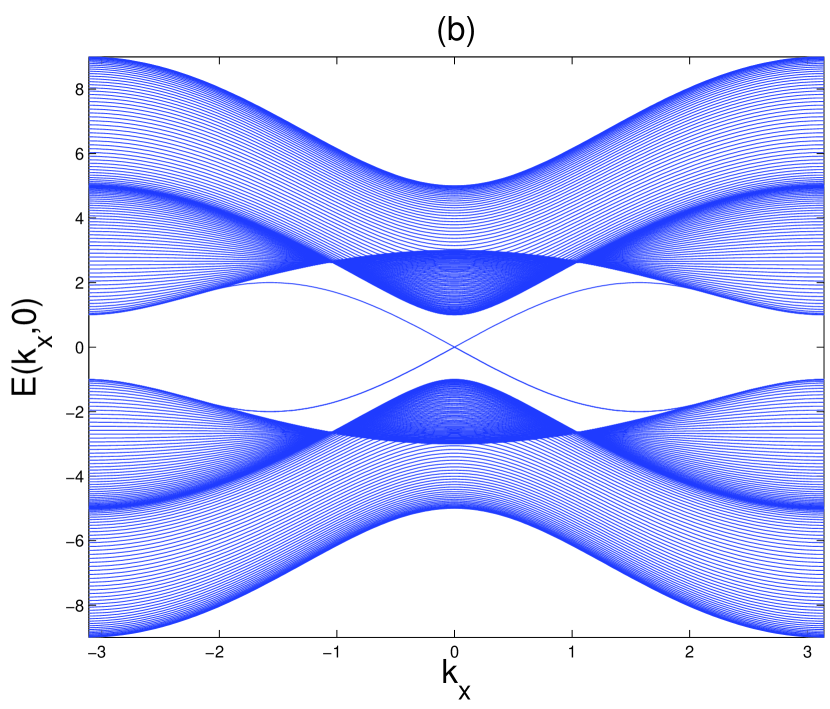
Figure 7: Numerical dispersions of bulk and surface states for model I with $V_{z}/M=0.6$ for (a) and (c) and $2.0$ for (b) and (d). In (a) and (b) $k_{z}=0$, and in (c) and (d) $k_{x}=0$. The other parameters are same as in figure 1

Figure 7 shows results for the energy dispersions with finite $V_{z}$ obtained from numerical calculations on a finite size system. One can see from the figure that the directions $k_{x}$ and $k_{z}$ differ. This is again due to the fact that $\Gamma_{z}$ commutes with $\Gamma_{I}^{3}$ but anticommutes with $\Gamma^{1}$. We see from the figure that a one dimensional flat band appears in $k_{z}$-direction if $V_{z}$ exeeds $M$.

5.5 Existence of a one-dimensional flat band

Similarly as in the case with nonzero $V_{x}$ the appearance of this one-dimensional flat band can be understood using the classification of Matsuura et al.[51] For that purpose we consider the Hamiltonian without the $\Gamma^{1}$ term:

$$H_{1}(\mathbf{k})=m_{0}(\mathbf{k})\Gamma^{0}+m_{2}(\mathbf{k})\Gamma^{2}+m_{3}(\mathbf{k})\Gamma_{I}^{3}+V_{z}\Gamma_{z}$$ (48)

If one considers this Hamiltonian for $k_{x}=0$ as a function of the two coordinates $k_{y}$ and $k_{z}$, its Fermi surface will be a point node in the two-dimensional Brillouin zone. However, one can also consider this Hamiltonian as a function of the three coordinates $k_{x}$, $k_{y}$, and $k_{z}$, keeping the $k_{x}$ dependence in $m_{0}(\mathbf{k})$. Then, its Fermi surface will be a line node in the three-dimensional Brillouin zone. In any case, $H_{1}$ belongs to class AIII due to the chiral symmetry $\Theta_{1}$. Using the chiral symmetry $\Theta_{1}$ we can bring $H_{1}$ into off-diagonal block form, similarly as in section 5.3:

$$H_{1}(\mathbf{k}) =\left(\begin{array}[]{cc}0&D_{1}^{\dagger}(\mathbf{k})\\ D_{1}(\mathbf{k})&0\end{array}\right),$$ (51)

where the block $D_{1}(\mathbf{k})$ is found to be

$$D_{1}(\mathbf{k})=\left(\begin{array}[]{cc}m_{0}(\mathbf{k})+im_{3}(\mathbf{k})&-im_{2}(\mathbf{k})-V_{z}\\ -im_{2}(\mathbf{k})-V_{z}&m_{0}(\mathbf{k})-im_{3}(\mathbf{k})\end{array}\right).$$ (52)

Using this block, we can again define the winding number

$$w(k_{x},k_{z})=\frac{1}{2\pi}\textrm{Im}\int_{-\pi}^{\pi}\,dk_{y}\,\partial_{k_{y}}\ln\textrm{det}D_{1}(\mathbf{k}).$$ (53)

Following the method outlined in appendix III we can derive an analytical condition for the existence of a flat band of $H_{1}$ which reads

$$|V_{z}|>\sqrt{\tilde{m}_{0}(\mathbf{k})^{2}+4A_{1}^{2}\sin^{2}(k_{z})}.$$ (54)

For $k_{x}=0$ this yields a range of $k_{z}$ values for which a one-dimensional flat band exists, consistent with the numerical result in Fig. 7. If we consider $H_{1}$ as a function of three coordinates $k_{x}$, $k_{y}$, and $k_{z}$, this condition tells us that $H_{1}$ actually possesses a two-dimensional surface flat band within a certain area in $(k_{x},k_{z})$-space. Now, $H=H_{1}+m_{1}\Gamma^{1}$ and $\Gamma^{1}$ anticommutes with $H_{1}$. This means that the zero energy states of $H_{1}$ are eigenstates of $\Gamma^{1}=\Theta_{1}$, too. As a result, the dispersion of the surface flat band of the full Hamiltonian $H$ is given by

$$E_{\pm}(k_{x},k_{z})=\pm 2A_{2}\sin k_{x}.$$ (55)

Thus, the surface state dispersions become highly anisotropic, being flat in $k_{z}$-direction, but dispersive in $k_{x}$-direction.

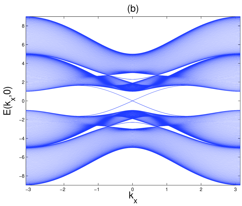
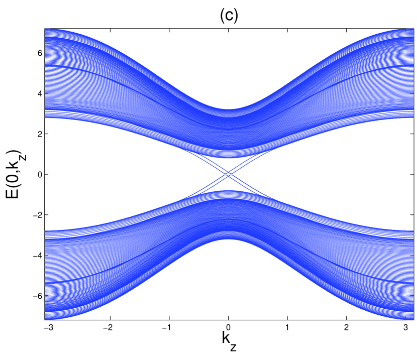
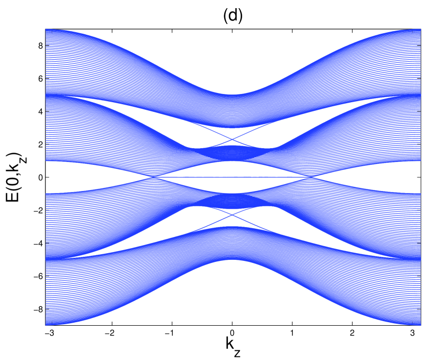
Figure 8: Numerical dispersions of bulk and surface states for model I with exchange fields $(V_{x},V_{y},V_{z})=0.2M(1/2,1/2,1/\sqrt{2})$ for (a) and (c) and $2.0M(1/2,1/2,1/\sqrt{2})$ for (b) and (d). In (a) and (b) $k_{z}=0$, and in (c) and (d) $k_{x}=0$. The other parameters are same as in figure 1

In Figure 8 we illustrate an example of the general case, where all three components of the exchange field are nonzero. One sees from the figure that at small fields the surface states are splitted, similarly as in Figure 1 (a) and (c). However, when the magnitude of the exchange field exceeds $M$, a one-dimensional flat band appears in $k_{z}$ direction, similarly as in Figure 7 (b) and (d).

In order to understand the appearance of a flat band in this general case let us consider the following partial bulk Hamiltonian:

$$H_{0}(\mathbf{k})=m_{0}({\mathbf{k}})\Gamma^{0}+m_{2}({\mathbf{k}})\Gamma^{2}+V_{x}\Gamma_{x}+V_{y}\Gamma_{y}+V_{z}\Gamma_{z}$$ (56)

We first construct a symmetry operator $\Theta_{13}$ that anticommutes with this $H_{0}$. We first note that the operator $\Theta_{1}$ anticommutes with $\Gamma^{0}$, $\Gamma^{2}$, $\Gamma_{y}$, and $\Gamma_{z}$, but commutes with $\Gamma_{x}$, while the operator $\Theta_{3}$ anticommutes with $\Gamma^{0}$, $\Gamma^{2}$, $\Gamma_{x}$, and $\Gamma_{y}$, but commutes with $\Gamma_{z}$. If we choose, however, the following linear superposition of $\Theta_{1}$ and $\Theta_{3}$

$$\Theta_{13}=\frac{V_{z}}{\sqrt{V_{x}^{2}+V_{z}^{2}}}\Theta_{1}-\frac{V_{x}}{\sqrt{V_{x}^{2}+V_{z}^{2}}}\Theta_{3}=\sin\chi\,\Theta_{1}-\cos\chi\,\Theta_{3}$$ (57)

it is easy to see that $\Theta_{13}$ anticommutes with the four operators $\Gamma^{0}$, $\Gamma^{2}$, $\Gamma_{y}$, and $V_{x}\Gamma_{x}+V_{z}\Gamma_{z}$. Here, we defined the angle $\chi$ via $V_{x}=V_{0}\cos\chi$ and $V_{z}=V_{0}\sin\chi$ with $V_{0}=\sqrt{V_{x}^{2}+V_{z}^{2}}$. Thus, the partial Hamiltonian $H_{0}$ possesses a chiral symmetry $\Theta_{13}$, which depends on the direction of the exchange field. For $V_{z}=0$ the symmetry operator reduces to $\Theta_{3}$, corresponding to the case in section 5.3 and for $V_{x}=0$ the symmetry reduces to the case discussed in section 5.5.

Using the chiral symmetry $\Theta_{13}$ we can bring $H_{0}$ into off-diagonal block form by transforming to the eigenbasis of $\Theta_{13}$. There are two eigenvectors of $\Theta_{13}$ with eigenvalue -1, which are $\eta_{1}=(0,0,\sin\frac{\chi}{2},\cos\frac{\chi}{2})^{T}$ and $\eta_{2}=(\cos\frac{\chi}{2},-\sin\frac{\chi}{2},0,0)^{T}$ and two eigenvectors with eigenvalue +1, which are $\eta_{3}=(\sin\frac{\chi}{2},\cos\frac{\chi}{2},0,0)^{T}$ and $\eta_{4}=(0,0,\cos\frac{\chi}{2},-\sin\frac{\chi}{2})^{T}$. In this basis $H_{0}$ becomes block off-diagonal

$$H_{0}(\mathbf{k}) =\left(\begin{array}[]{cc}0&D_{2}^{\dagger}(\mathbf{k})\\ D_{2}(\mathbf{k})&0\end{array}\right),$$ (60)

where the block $D_{2}(\mathbf{k})$ is

$$D_{2}(\mathbf{k})=\left(\begin{array}[]{cc}m_{0}&V_{0}+i(m_{2}+V_{y})\\ V_{0}+i(m_{2}-V_{y})&m_{0}\end{array}\right)$$ (61)

and its determinant

$$\mathrm{det}\;D_{2}(\mathbf{k})=m_{0}^{2}+m_{2}^{2}-V_{0}^{2}-V_{y}^{2}-2im_{2}V_{0}$$ (62)

The Hamiltonian $H_{0}$ possesses a two-dimensional zero energy surface flat band, if the corresponding winding number becomes nonzero. Following appendix III we find the criterion that

$$\left(V^{2}-\tilde{m}_{0}^{2}\right)\left(V^{2}-\left(\tilde{m}_{0}-4B_{2}\right)^{2}\right)<0$$ (63)

where $\tilde{m}_{0}(\mathbf{k})=M-2B_{2}(1-\cos k_{x})-2B_{1}(1-\cos k_{z})$. In the vicinity of $k_{x}=k_{z}=0$ this criterion can usually be fulfilled for $V>M$, if $V$ does not become too large.

Having seen that the partial Hamiltonian $H_{0}$ possesses a two-dimensional zero energy surface flat band we can apply

$$H^{\prime}(\mathbf{k})=m_{1}({\mathbf{k}})\Gamma^{1}+m_{3}({\mathbf{k}})\Gamma_{I}^{3}$$ (64)

as a perturbation to find the approximate surface state dispersion for the full Hamiltonian. For that purpose we need the surface state wave function $\psi_{s}$. As the zero energy state is a common eigenstate of $H_{0}$ and $\Theta_{13}$, $\psi_{s}$ will be a superposition of two eigenvectors of $\Theta_{13}$ with the same eigenvalue, like

$$\psi_{s}(y)=f_{1}(y)\eta_{1}+f_{2}(y)\eta_{2}$$ (65)

The two functions $f_{1}(y)$ and $f_{2}(y)$ have to be determined from the differential equation $H_{0}(k_{y}\rightarrow-i\partial_{y})\psi_{s}=0$ and are found to be superpositions of three exponentially decaying functions. An analogous superposition of the +1 eigenstates of $\Theta_{13}$ leads to exponentially increasing functions, which cannot fulfil the boundary conditions. They correspond to solutions localized at the opposite boundary. Both functions $f_{1}(y)$ and $f_{2}(y)$ fulfil $f_{1}(y=0)=f_{2}(y=0)=0$ and are normalized such that

$$\int_{0}^{\infty}dy\left|f_{1}(y)\right|^{2}+\int_{0}^{\infty}dy\left|f_{2}(y)\right|^{2}=1\;.$$ (66)

The energy of the perturbed system is given by

$$E=\left\langle\psi_{s}\left|m_{1}\Gamma^{1}+m_{3}\Gamma_{I}^{3}\right|\psi_{s}\right\rangle$$ (67)

By direct calculation we find that

$$\left\langle\eta_{i}\left|\Gamma_{I}^{3}\right|\eta_{j}\right\rangle=0\quad\mbox{for}\quad i,j\in\left\{1,2\right\}$$ (68)

and

$$\left\langle\eta_{i}\left|\Gamma^{1}\right|\eta_{j}\right\rangle=-\sin\chi\delta_{ij}=-\frac{V_{z}}{\sqrt{V_{x}^{2}+V_{z}^{2}}}\delta_{ij}\quad\mbox{for}\quad i,j\in\left\{1,2\right\}\;.$$ (69)

As a result we find for the energy of the surface states of the full Hamiltonian:

$$E(k_{x},k_{z})=-m_{1}\frac{V_{z}}{\sqrt{V_{x}^{2}+V_{z}^{2}}}=-\frac{V_{z}}{\sqrt{V_{x}^{2}+V_{z}^{2}}}2A_{2}\sin k_{x}$$ (70)

From this expression we see that for $V_{z}\neq 0$ we always have a one-dimensional flat band in $k_{z}$-direction. The group velocity in $x$-direction can be tuned by rotating the exchange field within the $xz$-plane and vanishes when $V_{z}$ becomes zero. This expression shows how the one-dimensional flat band develops into the two-dimensional flat band for exchange field within the $xy$-plane.

5.6 Weyl semimetal

In this section we show that the semimetallic state of model I for an exchange field $V>V_{cr}$ and $V_{z}\neq 0$ is actually a realization of a Weyl semimetal. The Weyl semimetallic phase can be viewed as a three-dimensional generalization of the two-dimensional Dirac electrons in graphene, as has been pointed out recently [52, 53, 54]. In contrast to graphene, just two linearly dispersing adjacent bands touch at a finite number of points in the three-dimensional Brillouin zone. In the vicinity of these Weyl nodes, which have also been termed “diabolic” points [66], the effective two-band Hamiltonian can be written in the form

$$H(\bf k) =\hbar v_{F}\left(k_{x}\sigma_{x}+k_{y}\sigma_{y}+k_{z}\sigma_{z}\right)$$ (71)

where the Pauli matrices $\sigma_{i}$ do not need to refer to the spin degree of freedom. Such a diabolic point is exceptionally stable due to topology, as arbitrary perturbations cannot remove it unless an annihilation with another diabolic point occurs. A recent theoretical work proposed the appearence of a Weyl semimetallic phase in pyrochlore iridates [52]. It was shown that the surface states of the Weyl semimetal may form open Fermi “arcs”, i.e. Fermi lines which terminate at the projection of the diabolic points onto the surface Brillouin zone.

In appendix I we showed that for $V>V_{cr}$ model I enters a semimetallic phase. If $V_{z}\neq 0$ the bulk spectrum indeed possesses either two or four Fermi points on the $k_{z}$-axis, where two bands touch each other. We still need to show that around these points the Hamiltonian can be written in a form like Eq. (71). In order to do so we use a similar technique as we have used for determination of the dispersion of the surface states. Let ${\mathbf{k}}_{0}=(0,0,k_{z,0})$ be the position of a Fermi point. We first consider the partial bulk Hamiltonian at ${\mathbf{k}}_{0}$

$$H_{0}(\mathbf{k})=m_{0}({\mathbf{k}}_{0})\Gamma^{0}+m_{3}({\mathbf{k}}_{0})\Gamma_{I}^{3}+V_{x}\Gamma_{x}+V_{y}\Gamma_{y}+V_{z}\Gamma_{z}$$ (72)

and construct a symmetry operator $\Theta_{12}$ that anticommutes with it. The zero energy eigenstates of $H_{0}$ are then simultaneous eigenstates of $\Theta_{12}$. From the eigenstates of $\Theta_{12}$ we determine the two zero energy eigenstates of $H_{0}$ at the Fermi point. We then expand the full Hamiltonian to lowest order in $k_{x}$, $k_{y}$, and $k_{z}-k_{z,0}$ around the Fermi points. This leads to a perturbation of the form

$$H^{\prime}(\mathbf{k}) =-2B_{1}\left(k_{z}-k_{z,0}\right)\sin k_{z,0}\Gamma^{0}+2A_{2}k_{x}\Gamma^{1}+2A_{2}k_{y}\Gamma^{2}+$$ (73)

$$+2A_{1}\left(k_{z}-k_{z,0}\right)\cos k_{z,0}\Gamma_{I}^{3}$$

The effective low energy $2\times 2$ Hamiltonian near the Fermi points is obtained by degenerate perturbation theory within the subspace of the two said eigenstates.

To construct the symmetry operator $\Theta_{12}$ we first note that the operator $\Theta_{1}$ anticommutes with $\Gamma^{0}$, $\Gamma_{I}^{3}$, $\Gamma_{y}$, and $\Gamma_{z}$, but commutes with $\Gamma_{x}$, while the operator $\Theta_{2}$ anticommutes with $\Gamma^{0}$, $\Gamma_{I}^{3}$, $\Gamma_{x}$, and $\Gamma_{z}$, but commutes with $\Gamma_{y}$. If we choose the following linear superposition of $\Theta_{1}$ and $\Theta_{2}$

$$\Theta_{12}=\frac{V_{y}}{\sqrt{V_{x}^{2}+V_{y}^{2}}}\Theta_{1}-\frac{V_{x}}{\sqrt{V_{x}^{2}+V_{y}^{2}}}\Theta_{2}=\sin\varphi\,\Theta_{1}-\cos\varphi\,\Theta_{2}$$ (74)

it is easy to see that $\Theta_{12}$ anticommutes with the four operators $\Gamma^{0}$, $\Gamma_{I}^{3}$, $\Gamma_{z}$, and $V_{x}\Gamma_{x}+V_{y}\Gamma_{y}$. There are two eigenvectors of $\Theta_{12}$ with eigenvalue -1, which are $\eta_{1}=(0,0,ie^{-i\varphi},1)^{T}$ and $\eta_{2}=(-ie^{-i\varphi},1,0,0)^{T}$ and two eigenvectors with eigenvalue +1, which are $\eta_{3}=(0,0,-ie^{-i\varphi},1)^{T}$ and $\eta_{4}=(ie^{-i\varphi},1,0,0)^{T}$. One of the two zero energy eigenstates of $H_{0}$ is a linear combination of $\eta_{1}$ and $\eta_{2}$, while the other one is a linear combination of $\eta_{3}$ and $\eta_{4}$. After a staightforward calculation which exploits the fact that at the Fermi points we have $m_{0}^{2}+m_{3}^{2}=V_{x}^{2}+V_{y}^{2}+V_{z}^{2}$ (see appendix I), we find the following eigenstates of $H_{0}$:

$$\psi_{1} =\frac{1}{2}\left(-ie^{-i\varphi},1,-e^{i(\chi-\varphi-\vartheta)},ie^{i(\chi-\vartheta)}\right)^{T}$$ (75)

$$\psi_{2} =\frac{1}{2}\left(-e^{-i(\varphi+\vartheta)},ie^{-i\vartheta},-ie^{i(\chi-\varphi)},e^{i\chi}\right)^{T}$$ (76)

where

$$e^{i\chi}=\frac{m_{0}+im_{3}}{\sqrt{m_{0}^{2}+m_{3}^{2}}}\quad\mbox{and}\quad e^{i\vartheta}=\frac{\sqrt{V_{x}^{2}+V_{y}^{2}}+iV_{z}}{\sqrt{V_{x}^{2}+V_{y}^{2}+V_{z}^{2}}}$$ (77)

To find the effective low energy $2\times 2$ Hamiltonian near the Fermi points for convenience we use the two basis states

$$\psi_{1}^{\prime}=\frac{1}{\sqrt{2}}\left(\psi_{1}+\psi_{2}\right)\quad\mbox{and}\quad\psi_{2}^{\prime}=\frac{1}{\sqrt{2}}\left(\psi_{1}-\psi_{2}\right)$$ (78)

In this basis the Hamiltonian $H^{\prime}$ becomes

$$H^{\prime} =\left[-2B_{1}\sin k_{z,0}\cos\chi+2A_{1}\cos k_{z,0}\sin\chi\right]\left(k_{z}-k_{z,0}\right)\sigma_{z}+$$ (79)

$$+2A_{2}k_{x}\left[-\sin\varphi\,\sigma_{x}+\cos\varphi\sin\vartheta\,\sigma_{y}\right]+$$

$$2A_{2}k_{y}\left[\cos\varphi\,\sigma_{x}+\sin\varphi\sin\vartheta\,\sigma_{y}\right]$$

Apparently, this is an anisotropic Weyl-type Hamiltonian. For example for $V_{x}=0$ this expression simplifies to

$$H^{\prime} =\left[-2B_{1}\sin k_{z,0}\cos\chi+2A_{1}\cos k_{z,0}\sin\chi\right]\left(k_{z}-k_{z,0}\right)\sigma_{z}+$$ (80)

$$-2A_{2}k_{x}\,\sigma_{x}+2A_{2}k_{y}\sin\vartheta\,\sigma_{y}$$

Having seen that model I for $V>V_{cr}$ and $V_{z}\neq 0$ is a Weyl semimetal we can see now that the one-dimensional surface flat band from the previous section Eq. (55) is just a Fermi “arc” in the sense of Ref. [52]. It exists only in a limited range of $k_{z}$ values given by Eq. (54). The end points of the Fermi arc are just the projections of the Weyl nodes onto the surface Brillouin zone $(k_{x},k_{z})$, as one sees by setting $k_{x}=0$ in Eq. (54) and comparison with Eqs. (117) and (124) in appendix I.

5.7 Boundary perpendicular to the $z$-direction

The case with a $z$-boundary is much easier to treat than the case with a $y$-boundary. In this case we can decompose the Hamiltonian in the following way:

$$H(\bf k) =H_{0}(\mathbf{k})+H^{\prime}(\mathbf{k}),$$

where

$$H_{0}(\mathbf{k}) =(\tilde{m}_{0}(\mathbf{k})+B_{1}\partial_{z}^{2})\Gamma^{0}+2A_{1}\partial_{z}\Gamma_{I}^{3},$$ (81)

$$H^{\prime}(\mathbf{k}) =m_{1}(\mathbf{k})\Gamma^{1}+m_{2}(\mathbf{k})\Gamma^{2}+V_{x}\Gamma_{x}+V_{y}\Gamma_{y}+V_{z}\Gamma_{z}.$$ (82)

Here, $\tilde{m}_{0}(\mathbf{k})=M-2B_{2}(1-\cos k_{x})-2B_{2}(1-\cos k_{y})$ and $\mathbf{k}=(k_{x},k_{y})$ now.

We are now in the lucky situation that $\Gamma_{x}$, $\Gamma_{y}$ and $\Gamma_{z}$ all commute with $H_{0}$, and both $\Gamma^{1}$ and $\Gamma^{2}$ anticommute with it. Thus, the surface states for an exchange field in arbitrary direction can be found from the zero energy surface states of $H_{0}$ using the method from appendix II.

We first determine the zero energy surface states of $H_{0}$ by noting that $H_{0}$ commutes with $\Gamma_{z}$ and anticommutes with the operator $\mathbb{I}_{2\times 2}\otimes\tau_{z}$. The common eigenstates of these two operators are just $(1,0,0,0)^{T}$, $(0,1,0,0)^{T}$, $(0,0,1,0)^{T}$, and $(0,0,0,1)^{T}$. We try the following two ansätze (the other two eigenstates leading to exponentially increasing functions again):

$$\psi_{1,\mathbf{k}}(y)=(1,0,0,0)^{T}f_{\mathbf{k}}(z),$$ (83)

$$\psi_{2,\mathbf{k}}(y)=(0,1,0,0)^{T}f_{\mathbf{k}}(z),$$ (84)

where $f_{\mathbf{k}}(z)$ is solution of the equation

$$[\tilde{m}_{0}(\mathbf{k})+B_{1}\partial_{z}^{2}+2A_{1}\partial_{z}]f_{\mathbf{k}}(z)=0,$$ (85)

Solving the differential equation (85) we find that $f_{\mathbf{k}}(z)$ is given by

$$f_{\mathbf{k}}(z)=e^{-\frac{A_{1}}{B_{1}}z}\sinh\left(\sqrt{\frac{A_{1}^{2}}{B_{1}^{2}}-\frac{\tilde{m}_{0}(\mathbf{k})}{B_{1}}}\;z\right).$$ (86)

This solution can only fulfil the boundary condition for $z\rightarrow\infty$, if $\tilde{m}_{0}(\mathbf{k})>0$. For those $\mathbf{k}$ values where this condition is not fulfilled anymore, a surface state does not exist. The form of the solutions Eq. (83) and (84) means that the surface state only occupies orbital 1, leaving orbital 2 empty. Correspondingly, the surface state at the opposite surface of the system is found to occupy orbital 2 only.

To obtain the surface states of $H$ from the ones of $H_{0}$ we have to determine those linear combinations of $\psi_{1,\mathbf{k}}$ and $\psi_{2,\mathbf{k}}$ that diagonalize $H^{\prime}$, i.e.

$$\Psi_{1,\mathbf{k}} =a_{1}(\mathbf{k})\psi_{1,\mathbf{k}}(z)+b_{1}(\mathbf{k})\psi_{2,\mathbf{k}}(z),$$ (87)

$$\Psi_{2,\mathbf{k}} =a_{2}(\mathbf{k})\psi_{1,\mathbf{k}}(z)+b_{2}(\mathbf{k})\psi_{2,\mathbf{k}}(z).$$ (88)

If we write $\xi_{i}(\mathbf{k})=(a_{i}(\mathbf{k}),b_{i}(\mathbf{k}))^{T}$ the coefficients are determined from the equation

$$[(V_{x}+m_{1}(\mathbf{k}))\sigma_{x}+(V_{y}+m_{2}(\mathbf{k}))\sigma_{y}+V_{z}\sigma_{z}]\xi_{1}(\mathbf{k})=E_{1}(\mathbf{k})\xi_{1}(\mathbf{k}).$$ (89)

The eigenenergies are given by

$$E_{1,\pm}(\mathbf{k})=\pm\sqrt{V_{z}^{2}+(2A_{2}\sin k_{x}+V_{x})^{2}+(2A_{2}\sin k_{y}+V_{y})^{2}}.$$ (90)

This expression tells us that the components of the exchange field parallel to the surface ($V_{x}$ and $V_{y}$) for small momenta just shift and split the surface Dirac cone without opening a gap and without changing the group velocity. The component $V_{z}$ perpendicular to the surface opens a gap, however. This behavior is in agreement with previous work [20]. A flat band does not appear in this geometry. Even though the system is still a Weyl semimetal in the bulk, a surface Fermi arc does not appear, because the Weyl nodes all sit on the $k_{z}$-axis. Thus, their projection onto the surface Brillouin zone is the single point $k_{x}=k_{y}=0$ and the Fermi arc is not present.

The full surface state wave functions can be written in the form

$$\Psi_{+,\mathbf{k}}(y) =\left(e^{-i\phi_{\mathbf{k}}}\cos\frac{\theta_{\mathbf{k}}}{2},\sin\frac{\theta_{\mathbf{k}}}{2},0,0\right)^{T}f_{\mathbf{k}}(z)$$ (91)

$$\Psi_{-,\mathbf{k}}(y) =\left(-e^{-i\phi_{\mathbf{k}}}\sin\frac{\theta_{\mathbf{k}}}{2},\cos\frac{\theta_{\mathbf{k}}}{2},0,0\right)^{T}f_{\mathbf{k}}(z)$$ (92)

Here, we have introduced two spherical angles $\phi$ and $\theta$ that define the direction of the vector $(m_{1}+V_{x},m_{2}+V_{y},V_{z})$:

$$\cos\phi_{\mathbf{k}}\sin\theta_{\mathbf{k}} =\frac{2A_{2}\sin k_{x}+V_{x}}{\sqrt{V_{z}^{2}+(2A_{2}\sin k_{x}+V_{x})^{2}+(2A_{2}\sin k_{y}+V_{y})^{2}}}$$

$$\sin\phi_{\mathbf{k}}\sin\theta_{\mathbf{k}} =\frac{2A_{2}\sin k_{y}+V_{y}}{\sqrt{V_{z}^{2}+(2A_{2}\sin k_{x}+V_{x})^{2}+(2A_{2}\sin k_{y}+V_{y})^{2}}}$$

$$\cos\theta_{\mathbf{k}} =\frac{V_{z}}{\sqrt{V_{z}^{2}+(2A_{2}\sin k_{x}+V_{x})^{2}+(2A_{2}\sin k_{y}+V_{y})^{2}}}$$

For the spin texture of these surface states we find

$$\left\langle\Psi_{\pm,\mathbf{k}}\left|\hat{s}_{1,x}\right|\Psi_{\pm,\mathbf{k}}\right\rangle =\pm\cos\phi_{\mathbf{k}}\sin\theta_{\mathbf{k}}$$

$$\left\langle\Psi_{\pm,\mathbf{k}}\left|\hat{s}_{1,y}\right|\Psi_{\pm,\mathbf{k}}\right\rangle =\pm\sin\phi_{\mathbf{k}}\sin\theta_{\mathbf{k}}$$

$$\left\langle\Psi_{\pm,\mathbf{k}}\left|\hat{s}_{1,z}\right|\Psi_{\pm,\mathbf{k}}\right\rangle =\pm\cos\theta_{\mathbf{k}}$$

The spin in orbital 2 vanishes. This means that the spin is directed along the vector $(m_{1}+V_{x},m_{2}+V_{y},V_{z})$. For $V_{z}=0$ the spin-$z$ component vanishes and the spin is oriented within the plane of the surface, in contrast to the cases with the $y$-boundary.

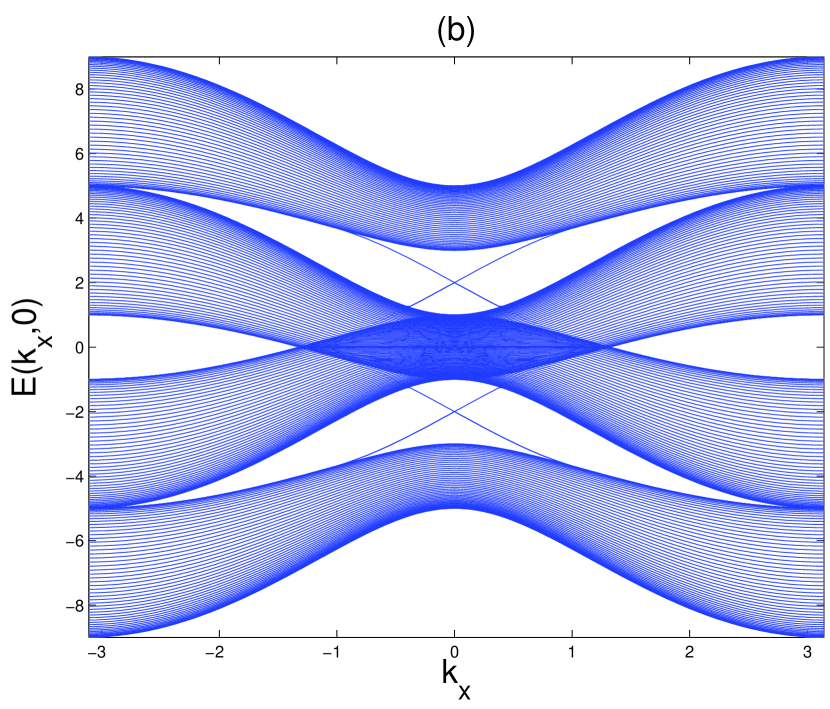
Figure 9: Numerical dispersions of bulk and surface states for model I with boundary in $z$-direction for $V_{x}/M=0.2$ in (a) and (c) and $2.0$ in (b) and (d). In (a) and (b) $k_{y}=0$, and in (c) and (d) $k_{x}=0$. The other parameters are same as in figure 1

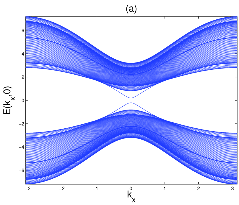
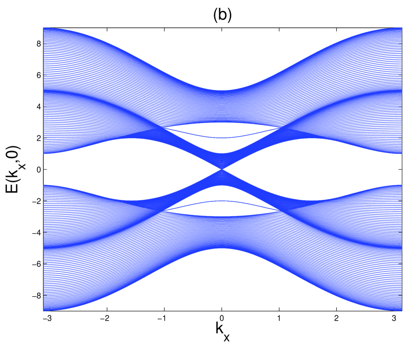
Figure 10: Numerical dispersions of bulk and surface states for model I with boundary in $z$-direction for $V_{z}/M=0.2$ in (a) and (c) and $2.0$ in (b) and (d). In (a) and (b) $k_{y}=0$, and in (c) and (d) $k_{x}=0$. The other parameters are same as in figure 1

Figure 9 shows numerical dispersions from a finite size system with finite $V_{x}$ in agreement with Eq. (90). For larger values of the exchange field $V_{x}>M$ the bulk gap has closed. The surface states then exist within the bulk bands.

Figure 10 shows numerical dispersions with finite $V_{z}$ confirming the opening of a gap for small values of $V_{z}$. Again, for larger values of the exchange field $V_{z}>M$ the surface states only exist within the bulk bands and no flat band appears.

6 Model II

In this section we discuss the two nonequivalent cases for the particle-hole symmetric model II. Model II is distinguished from model I only in the coupling in $k_{z}$-direction by the matrix $\Gamma_{II}^{3}=\sigma_{z}\otimes\tau_{z}$ instead of $\Gamma_{I}^{3}$. The other $\Gamma$-matrices are the same as in model I. The matrix $\Gamma_{II}^{3}$ has different commutation and anti-commutation relations than $\Gamma_{I}^{3}$. Model II is more symmetric in the sense, that the three spatial directions possess equivalent couplings. Therefore, it does not matter which direction of the boundary we consider. For convenience we choose a boundary in $y$-direction, because this allows us to build on the results from model I found in the previous section.

6.1 Finite $V_{x}$ and $V_{y}$

The case with both $V_{x}$ and $V_{y}$ nonzero, but $V_{z}=0$ can be treated along the same lines as has been discussed for model I in section 5.2. We can again go over to polar coordinates in this case and write $V_{x}=V_{0}\cos\vartheta$ and $V_{y}=V_{0}\sin\vartheta$. The bulk energy bands Eq. (3) can then be brought into the form:

$$E_{i}^{II}(\mathbf{k}) =\pm\Big{\{}\left(m_{1}\sin\vartheta-m_{2}\cos\vartheta\right)^{2}+m_{3}^{2}+$$ (93)

$$+\left(V_{0}\pm\sqrt{m_{0}^{2}+\left(m_{1}\cos\vartheta+m_{2}\sin\vartheta\right)^{2}}\right)^{2}\Big{\}}^{1/2}$$

Again, the system is insulating in the absence of an exchange field and the gap closes, when $V_{0}$ reaches a critical value $V_{cr}\sim M$. In contrast to model I, in model II $V_{cr}$ depends on the direction of the exchange field as detailed in appendix I. In the semimetallic state the Fermi surface is defined by three equations $m_{1}\sin\vartheta-m_{2}\cos\vartheta=0$, $m_{3}=0$, and $V_{0}^{2}=m_{0}^{2}+\left(m_{1}\cos\vartheta+m_{2}\sin\vartheta\right)^{2}$ now. Therefore, the Fermi surface is pointlike, i.e. zero-dimensional. Similarly as in section 5.6 it can be shown by linearization around the point nodes that the system is a Weyl semimetal in this case, too.

To determine the surface states, we can start from the same Hamiltonian $H_{0}^{\prime}$ in Eq. (25) and its zero energy surface states in Eq. (26) and (27). We can then treat the terms

$$H^{\prime}(\mathbf{k})=m_{1}(\mathbf{k})\Gamma^{1}+m_{3}(\mathbf{k})\Gamma_{II}^{3}+V_{y}\Gamma_{y}.$$ (94)

using degenerate perturbation theory again. In contrast to the matrix $\Gamma_{I}^{3}$ the matrix $\Gamma_{II}^{3}$ leads to a diagonal coupling of the two surface states instead of an off-diagonal coupling. As a result the dispersion of the surface states in $k_{z}$-direction remains unaffected by the spatial overlap $\beta(V_{x},\mathbf{k})$ Eq. (30). Consequently, we find the following surface state dispersions for the full Hamiltonian within perturbation theory:

$$E_{\pm}(\mathbf{k})=\pm\sqrt{\beta(V_{x},\mathbf{k})^{2}\left(V_{y}^{2}+4A_{2}^{2}\sin^{2}k_{x}\right)+4A_{1}^{2}\sin^{2}k_{z}}.$$ (95)

This dispersion shows that the $V_{y}$ component of the exchange field, which is perpendicular to the surface, opens a gap in the surface state spectrum for small values of $V_{y}$. The component $V_{x}$ parallel to the surface leads to an anisotropic reduction of the dispersion in $k_{x}$-direction, but not in $k_{z}$-direction. In Figures 11 and 12 we show the corresponding numerical results on a finite lattice for $V_{x}$ nonzero and $V_{y}$ nonzero, respectively, which agree with this behavior.

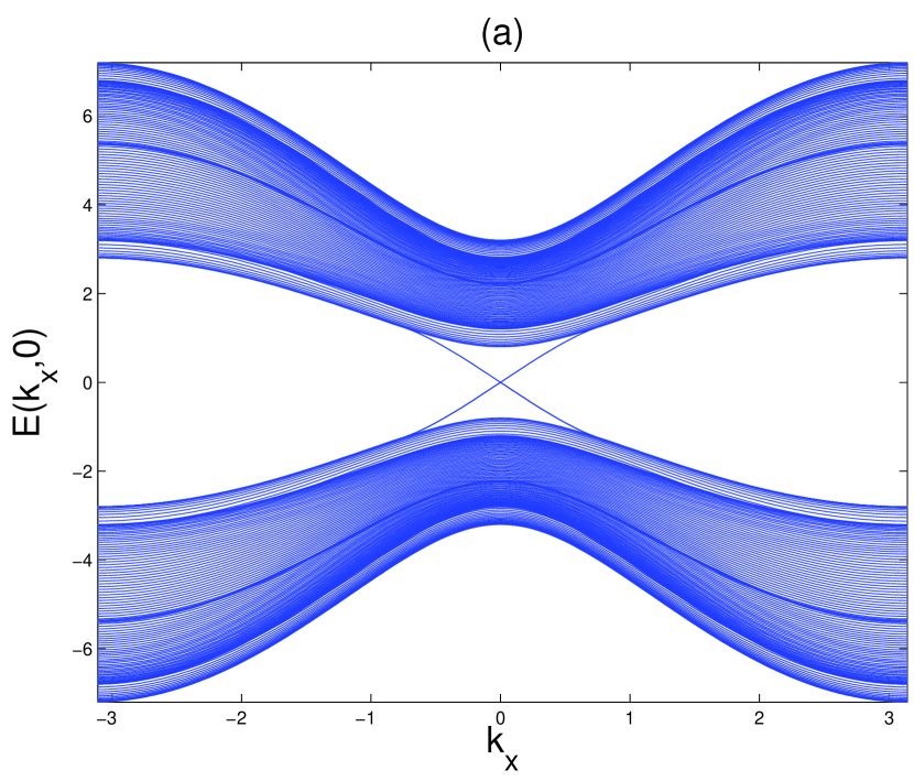
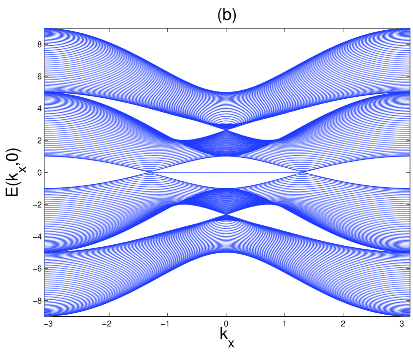
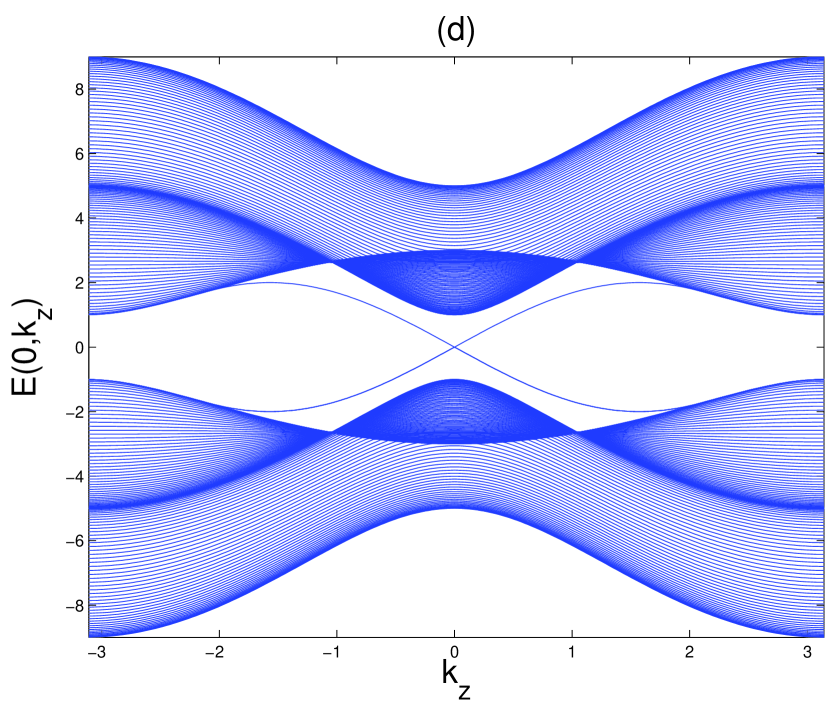
Figure 11: Numerical dispersions of bulk and surface states for model II with $V_{x}/M=0.2$ in (a) and (c) and $2.0$ in (b) and (d). In (a) and (b) $k_{z}=0$, and in (c) and (d) $k_{x}=0$. The other parameters are same as in figure 1

The surface state wave functions for this case can be written in the form

$$\Psi_{+,\mathbf{k}}(y) =e^{-i\phi_{\mathbf{k}}}\cos\frac{\theta_{\mathbf{k}}}{2}\psi_{1,\mathbf{k}}(y)+\sin\frac{\theta_{\mathbf{k}}}{2}\psi_{2,\mathbf{k}}(y)$$ (96)

$$\Psi_{-,\mathbf{k}}(y) =-e^{-i\phi_{\mathbf{k}}}\sin\frac{\theta_{\mathbf{k}}}{2}\psi_{1,\mathbf{k}}(y)+\cos\frac{\theta_{\mathbf{k}}}{2}\psi_{2,\mathbf{k}}(y)$$ (97)

Here, we have introduced two spherical angles $\phi_{\mathbf{k}}$ and $\theta_{\mathbf{k}}$ that define the direction of the vector $(\beta m_{1},\beta V_{y},m_{3})$:

$$\cos\phi_{\mathbf{k}}\sin\theta_{\mathbf{k}} =\frac{2\beta A_{2}\sin k_{x}}{\sqrt{\beta^{2}V_{y}^{2}+4\beta^{2}A_{2}^{2}\sin^{2}k_{x}+4A_{1}^{2}\sin k_{z}}}$$

$$\sin\phi_{\mathbf{k}}\sin\theta_{\mathbf{k}} =\frac{\beta V_{y}}{\sqrt{\beta^{2}V_{y}^{2}+4\beta^{2}A_{2}^{2}\sin^{2}k_{x}+4A_{1}^{2}\sin k_{z}}}$$

$$\cos\theta_{\mathbf{k}} =\frac{2A_{1}\sin k_{z}}{\sqrt{\beta^{2}V_{y}^{2}+4\beta^{2}A_{2}^{2}\sin^{2}k_{x}+4A_{1}^{2}\sin k_{z}}}$$

For the spin texture of these surface states we find in orbital 1:

$$\left\langle\Psi_{\pm,\mathbf{k}}\left|\hat{s}_{1,x}\right|\Psi_{\pm,\mathbf{k}}\right\rangle =\pm\frac{\beta}{2}\cos\phi_{\mathbf{k}}\sin\theta_{\mathbf{k}}$$

$$\left\langle\Psi_{\pm,\mathbf{k}}\left|\hat{s}_{1,y}\right|\Psi_{\pm,\mathbf{k}}\right\rangle =\pm\frac{\beta}{2}\sin\phi_{\mathbf{k}}\sin\theta_{\mathbf{k}}$$

$$\left\langle\Psi_{\pm,\mathbf{k}}\left|\hat{s}_{1,z}\right|\Psi_{\pm,\mathbf{k}}\right\rangle =\pm\frac{1}{2}\cos\theta_{\mathbf{k}}$$

In orbital 2 the $x$- and $z$-components of the spin turn out to be inverse:

$$\left\langle\Psi_{\pm,\mathbf{k}}\left|\hat{s}_{2,x}\right|\Psi_{\pm,\mathbf{k}}\right\rangle =\mp\frac{\beta}{2}\cos\phi_{\mathbf{k}}\sin\theta_{\mathbf{k}}$$

$$\left\langle\Psi_{\pm,\mathbf{k}}\left|\hat{s}_{2,y}\right|\Psi_{\pm,\mathbf{k}}\right\rangle =\pm\frac{\beta}{2}\sin\phi_{\mathbf{k}}\sin\theta_{\mathbf{k}}$$

$$\left\langle\Psi_{\pm,\mathbf{k}}\left|\hat{s}_{2,z}\right|\Psi_{\pm,\mathbf{k}}\right\rangle =\mp\frac{1}{2}\cos\theta_{\mathbf{k}}$$

Here, we see that in contrast to the corresponding case for model I the spin possesses components in all three spatial directions. In the limit $V_{y}\rightarrow 0$, the angle $\phi_{\mathbf{k}}$ goes to zero and the spin-$y$ component vanishes. The spatial overlap factor $\beta$ is seen to suppress only the $x$- and $y$-components of the spin. For the total spin we find:

$$\left\langle\Psi_{\pm,\mathbf{k}}\left|\Gamma_{x}\right|\Psi_{\pm,\mathbf{k}}\right\rangle =0$$

$$\left\langle\Psi_{\pm,\mathbf{k}}\left|\Gamma_{y}\right|\Psi_{\pm,\mathbf{k}}\right\rangle =\pm\beta\sin\phi_{\mathbf{k}}\sin\theta_{\mathbf{k}}$$

$$\left\langle\Psi_{\pm,\mathbf{k}}\left|\Gamma_{z}\right|\Psi_{\pm,\mathbf{k}}\right\rangle =0$$

The total spin is directed perpendicular to the surface. It vanishes in the limit $V_{y}\rightarrow 0$.

Figure 12: Numerical dispersions of bulk and surface states for model II with $V_{y}/M=0.2$ in (a) and (c) and $2.0$ in (b) and (d). In (a) and (b) $k_{z}=0$, and in (c) and (d) $k_{x}=0$. The other parameters are same as in figure 1

From the numerical results in Fig. 11 (b) and (d) we see that a one-dimensional flat band appears for nonzero $V_{x}>M$. Again, the appearence of this flat band can be understood by a topological winding number. In the present case the system obeys the chiral symmetry $\Theta_{3}$ for $k_{z}=0$, as was discussed in section 3. The Fermi surface is zero dimensional, so we may expect a one-dimensional flat band. As the Hamiltonians for model I and model II are identical for $k_{z}=0$, the off-diagonal block form of the Hamiltonian is the same as in Eq. (34), i.e.

$$D(\mathbf{k})=\left(\begin{array}[]{cc}m_{0}(\mathbf{k})&-m_{1}(\mathbf{k})+im_{2}(\mathbf{k})+V_{x}-iV_{y}\\ m_{1}(\mathbf{k})+im_{2}(\mathbf{k})+V_{x}+iV_{y}&m_{0}(\mathbf{k})\end{array}\right).$$ (98)

The corresponding winding number is then given by

$$w(k_{x})=\frac{1}{2\pi}\textrm{Im}\int_{-\pi}^{\pi}\,dk_{y}\,\partial_{k_{y}}\ln\textrm{det}D(\mathbf{k}).$$ (99)

The one-dimensional flat band in the present case thus corresponds to a $k_{z}=0$ cut of the flat band area shown in Fig. 5 (a). We can find the full dispersion of this flat band also for finite $k_{z}$ by noting that the matrix $\Gamma_{II}^{3}$ anticommutes with the Hamiltonian for $k_{z}=0$. As a result the zero energy states for $k_{z}=0$ are eigenstates of $\Gamma_{II}^{3}$, too. Therefore, the dispersion of the surface flat band for finite $k_{z}$ is given by

$$E_{\pm}(\mathbf{k})=\pm 2A_{1}\sin k_{z}.$$ (100)

Like for model I the zero energy surface of this one-dimensional flat band is a Fermi arc, whose end points are the projections of the Weyl nodes onto the surface Brillouin zone.

6.2 Finite $V_{z}$ and $V_{y}$

The case with both $V_{z}$ and $V_{y}$ nonzero, but $V_{x}=0$ can be treated like the corresponding case for model I in section 5.4. The Fermi surface turns out to be zero-dimensional and the system possesses the chiral symmetry $\Theta_{1}$ for $k_{x}=0$. For determination of the surface states we can start from the zero energy surface states Eqs. (43) and (44) of the Hamiltonian Eq. (39) and treat $H^{\prime}=m_{1}\Gamma^{1}+m_{3}\Gamma_{II}^{3}+V_{y}\Gamma_{y}$ as a perturbation. The energies of the surface states are then found to be

$$E_{\pm}(\mathbf{k})=\pm\sqrt{\beta(V_{z},\mathbf{k})^{2}\left(V_{y}^{2}+4A_{1}^{2}\sin^{2}k_{z}\right)+4A_{2}^{2}\sin^{2}k_{x}}.$$ (101)

This is the same kind of dispersion as in Eq. (95) with the roles of the $x$- and $z$-coordinates interchanged. The spin texture of the surface states in orbital 1 is found to be:

$$\left\langle\Psi_{\pm,\mathbf{k}}\left|\hat{s}_{1,x}\right|\Psi_{\pm,\mathbf{k}}\right\rangle =\pm\frac{1}{2}\frac{m_{1}}{\sqrt{m_{1}^{2}+\beta^{2}\left(m_{3}^{2}+V_{y}^{2}\right)}}$$

$$\left\langle\Psi_{\pm,\mathbf{k}}\left|\hat{s}_{1,y}\right|\Psi_{\pm,\mathbf{k}}\right\rangle =\pm\frac{1}{2}\frac{\beta V_{y}}{\sqrt{m_{1}^{2}+\beta^{2}\left(m_{3}^{2}+V_{y}^{2}\right)}}$$

$$\left\langle\Psi_{\pm,\mathbf{k}}\left|\hat{s}_{1,z}\right|\Psi_{\pm,\mathbf{k}}\right\rangle =\pm\frac{1}{2}\frac{\beta m_{3}}{\sqrt{m_{1}^{2}+\beta^{2}\left(m_{3}^{2}+V_{y}^{2}\right)}}$$

and in orbital 2:

$$\left\langle\Psi_{\pm,\mathbf{k}}\left|\hat{s}_{2,x}\right|\Psi_{\pm,\mathbf{k}}\right\rangle =\mp\frac{1}{2}\frac{m_{1}}{\sqrt{m_{1}^{2}+\beta^{2}\left(m_{3}^{2}+V_{y}^{2}\right)}}$$

$$\left\langle\Psi_{\pm,\mathbf{k}}\left|\hat{s}_{2,y}\right|\Psi_{\pm,\mathbf{k}}\right\rangle =\pm\frac{1}{2}\frac{\beta V_{y}}{\sqrt{m_{1}^{2}+\beta^{2}\left(m_{3}^{2}+V_{y}^{2}\right)}}$$

$$\left\langle\Psi_{\pm,\mathbf{k}}\left|\hat{s}_{2,z}\right|\Psi_{\pm,\mathbf{k}}\right\rangle =\mp\frac{1}{2}\frac{\beta m_{3}}{\sqrt{m_{1}^{2}+\beta^{2}\left(m_{3}^{2}+V_{y}^{2}\right)}}$$

For the total spin we find:

$$\left\langle\Psi_{\pm,\mathbf{k}}\left|\Gamma_{x}\right|\Psi_{\pm,\mathbf{k}}\right\rangle =0$$

$$\left\langle\Psi_{\pm,\mathbf{k}}\left|\Gamma_{y}\right|\Psi_{\pm,\mathbf{k}}\right\rangle =\pm\frac{\beta V_{y}}{\sqrt{m_{1}^{2}+\beta^{2}\left(m_{3}^{2}+V_{y}^{2}\right)}}$$

$$\left\langle\Psi_{\pm,\mathbf{k}}\left|\Gamma_{z}\right|\Psi_{\pm,\mathbf{k}}\right\rangle =0$$

The total spin is again directed perpendicular to the surface and vanishes in the limit $V_{y}\rightarrow 0$.

We find a one-dimensional flat band for finite $V_{z}>M$, that can be understood by a topological winding number using the chiral symmetry $\Theta_{1}$ for $k_{x}=0$, analogously to the previous case. As the matrix $\Gamma_{1}$ anticommutes with the Hamiltonian for $k_{x}=0$ we eventually find the dispersion of the surface flat band in this case as

$$E_{\pm}(\mathbf{k})=\pm 2A_{2}\sin k_{x}.$$ (102)

Again, the zero energy surface of this one-dimensional flat band is a Fermi arc, whose end points are the projections of the Weyl nodes onto the surface Brillouin zone.

7 Effect of broken particle-hole symmetry

So far we have studied the case $C=D_{1}=D_{2}=0$. When these parameters become nonzero, the particle-hole symmetry of the system is broken. Also, the chiral symmetries discussed in section 3 are not obeyed anymore. For this reason the topological winding numbers that we used in the previous sections to determine the presence or absence of a surface flat band cannot be used anymore. However, this does not mean that the surface bands completely disappear. In the following we will demonstrate by both numerical and analytical calculation that surface bands, which are energetically well separated from the bulk bands still exist in the broken particle-hole case. We will see that the surface bands become dispersive now with the dispersion increasing proportional to $D_{1}$ and $D_{2}$. Similar behavior has been noted in other systems before as well [51, 30, 32]. For the numerical calculations we use parameters that are realistic for Bi₂Se₃ and have been given in Ref. [56]. The Hamiltonian is now

$$H(\mathbf{k})=\epsilon_{0}(\mathbf{k})\mathbb{I}_{4\times 4}+\sum_{i=0}^{3}m_{i}(\mathbf{k})\Gamma^{i}+\sum_{\alpha\in\{x,y,z\}}V_{\alpha}\Gamma_{\alpha}$$ (103)

with $\epsilon_{0}(\mathbf{k})=C+2D_{2}(1-\cos k_{x})+2D_{2}(1-\cos k_{y})+2D_{1}(1-\cos k_{z})$, $m_{0}(\mathbf{k})=M-2B_{2}(1-\cos k_{x})-2B_{2}(1-\cos k_{y})-2B_{1}(1-\cos k_{z})$, $m_{1}(\mathbf{k})=2A_{2}\sin k_{x}$, $m_{2}(\mathbf{k})=2A_{2}\sin k_{y}$, and $m_{3}(\mathbf{k})=2A_{1}\sin k_{z}$. For Bi₂Se₃ parameters derived from Ref. [56] are: $A_{1}=0.575\,\textrm{eV}$, $A_{2}=0.495\,\textrm{eV}$, $B_{1}=2.74\,\textrm{eV}$, $B_{2}=3.30\,\textrm{eV}$, $C=-0.0068\,\textrm{eV}$, $D_{1}=0.36\,\textrm{eV}$, $D_{2}=1.14\,\textrm{eV}$, and $M=0.28\,\textrm{eV}$. Here, we have used the lattice constants $a=4.14$ Å  and $15c=28.64$ Å  for conversion into our lattice model. In the following, we use the same parameters for both model I and II.

It is clear that the bulk energy bands are just shifted by $\epsilon_{0}(\mathbf{k})$ with respect to the particle-hole symmetric cases studied in the previous sections. The former zero energy points, at which two bulk bands touch each other, will then have energy $\epsilon_{0}(\mathbf{k})$. For model I with $V_{z}=0$ and $V>V_{cr}$ we had a one-dimensional Fermi surface, whose degeneracy will now be lifted. Thus, these nodes will generally overlap with the two touching bulk bands. However, for the particle-hole symmetric model I with $V_{z}\neq 0$ and $V>M$ we have a Weyl semimetal with just two Fermi points. As these two Weyl nodes sit at symmetry related momentum points, they are shifted by the same amount $\epsilon_{0}(\mathbf{k})$. Therefore, the particle-hole broken system remains a Weyl semimetal unless the dispersion $\epsilon_{0}(\mathbf{k})$ becomes so large that the Weyl nodes start to overlap with the bulk bands. This same argument also holds for model II with $V>M$. Thus, the Weyl semimetallic phases in model I and II are preserved under not too large particle-hole symmetry breaking and we may still expect the presence of surface Fermi arcs, as we will show explicitly from our numerical calculations below. In the following we restrict the discussion to the geometries in which we found surface flat bands for the particle-hole symmetric cases.

7.1 Model I with boundary perpendicular to the $y$-direction

In the absence of an exchange field the surface state dispersions can be found by replacing the momentum $k_{y}$ by the momentum operator $-i\partial_{y}$ and solving the $4\times 4$ matrix Schrödinger equation directly with an exponential ansatz following Ref. [58]. This way one finds

$$E_{\pm}(\mathbf{k}) =C+Mt_{2}+2(D_{1}-B_{1}t_{2})(1-\cos k_{z})$$ (104)

$$\pm\sqrt{1-t_{2}^{2}}\sqrt{4A_{2}^{2}\sin^{2}k_{x}+4A_{1}^{2}\sin^{2}k_{z}},$$

where $t_{2}=D_{2}/B_{2}\approx 0.35$. If $t_{2}>1$ surface states do not exist.

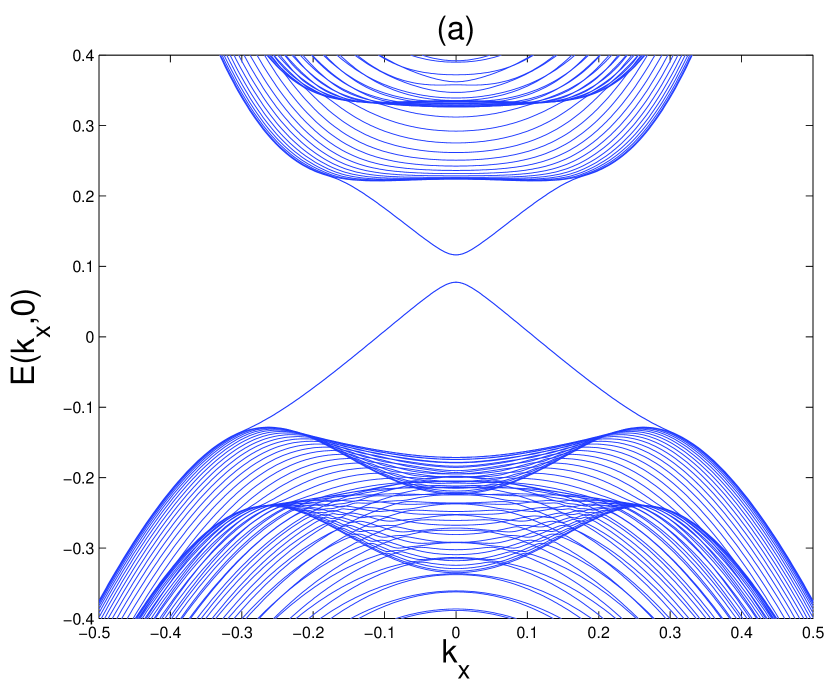
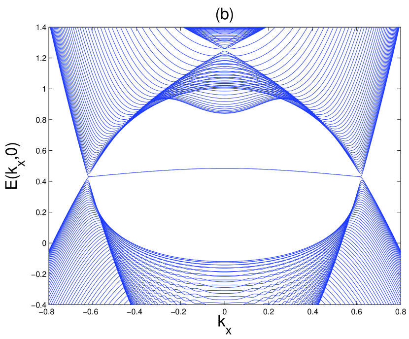
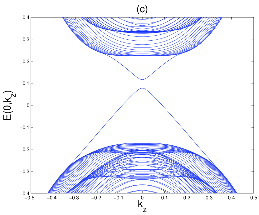
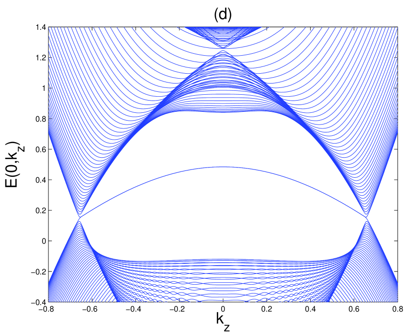
Figure 13: Numerical dispersions of bulk and surface states for model I with $V_{x}/M=0.2$ in (a) and (c) and $4.0$ in (b) and (d). In (a) and (b) $k_{z}=0$, and in (c) and (d) $k_{x}=0$. The other parameters are the ones for Bi₂Se₃ as described in the text.

When an exchange field is turned on, the Schrödinger equation leads to 8th order polynomials, whose zeroes cannot be given in closed form. However, analytical results can be obtained for fields in high symmetry directions and small values of momentum $k_{x}$ and $k_{z}$ by expansion.

When the exchange field points into $y$-direction we find the following dispersions

$$E_{\pm}(\mathbf{k}) =C+Mt_{2}+2(D_{1}-B_{1}t_{2})(1-\cos k_{z})$$ (105)

$$\pm\sqrt{\beta^{2}_{3}(k_{z})A_{2}^{2}\sin^{2}k_{x}+(V_{y}-\sqrt{1-t_{2}^{2}}A_{1}\sin k_{z})^{2}}.$$

Here, $\beta_{3}$ is a spatial overlap factor of the form

$$\beta_{3}(k_{z})=\frac{2A_{2}^{2}\sqrt{\left[M-2B_{1}\left(1-\cos k_{z}\right)\right]^{2}-4\frac{t_{2}^{2}}{1-t_{2}^{2}}A_{1}^{2}\sin^{2}k_{z}}}{2A_{2}^{2}\left[M-2B_{1}\left(1-\cos k_{z}\right)\right]+t_{2}^{2}B_{2}A_{1}^{2}\sin^{2}k_{z}}$$ (106)

Eq. (105) tells us that the Dirac cone remains ungapped for an exchange field in $y$-direction and is shifted in $k_{z}$ direction, like in the particle-hole symmetric case in section 5.1.

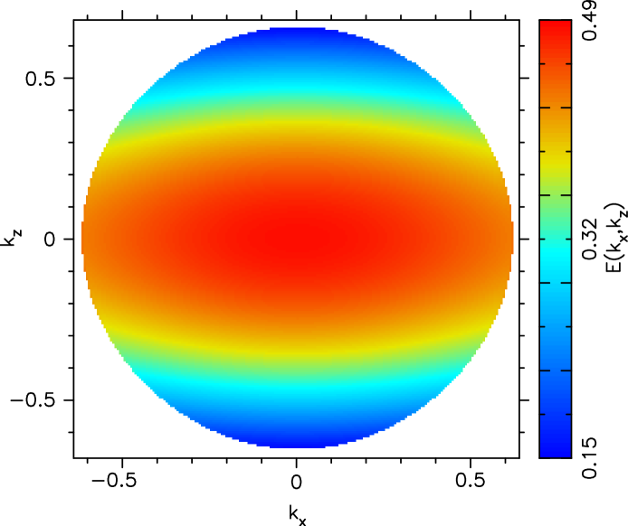
Figure 14: Dispersion of the surface band for model I with $V_{x}/M=4.0$. Red color indicates high energy values and blue color low values. The other parameters are the same as in figure 13

With exchange field in $x$-direction the following low field dispersions are found

$$E_{\pm}(\mathbf{k}) =C+Mt_{2}+2(D_{1}-B_{1}t_{2})(1-\cos k_{z})$$ (107)

$$\pm\sqrt{t_{2}^{2}V_{x}^{2}+\left(1-t_{2}^{2}\right)\beta^{2}_{4}(V_{x})\left(4A_{2}^{2}\sin^{2}k_{x}+4A_{1}^{2}\sin^{2}k_{z}\right)},$$

where the spatial overlap

$$\beta_{4}(V_{x})=\frac{4A_{2}^{2}\sqrt{M^{2}-V_{x}^{2}}}{4A_{2}^{2}M+\left(1-t_{2}^{2}\right)B_{2}V_{x}^{2}}$$ (108)

In contrast to Eq. (29) we now find the opening of a gap in the dispersion, which is of the order of $t_{2}V_{x}$. Corresponding numerical results on a finite lattice for $V_{x}=0.2M$ are shown in Fig. 13 (a) and (c). If we increase $V_{x}$ beyond $M$, we enter a state that corresponds to the two-dimensional flat band state discussed in section 5.3. As one can see in Fig. 13 (b) and (d) the surface band becomes dispersive now. However, it still exists and remains well separated from the two bulk bands. The dispersion of the surface band over the surface Brillouin zone is shown in color coded scale in Fig. 14. The dispersion is much smaller along $k_{x}$-direction than in $k_{z}$-direction. An approximate analytical expression valid for small $k_{x}$ and $k_{z}$ can be obtained from Eq. (107), if one sets $\beta_{4}=0$. In the total density of states of this system the surface band appears as a peak, similar to what was found for the edge states in a two-dimensional system in our previous work (see Fig. 5 in Ref. [24]).

With exchange field in $z$-direction we find the dispersions

$$E_{\pm}(\mathbf{k})=C+Mt_{2}+2(D_{1}-B_{1}t_{2})(1-\cos k_{z})$$ (109)

$$\pm\sqrt{4\beta^{2}_{5}(V_{z})\left(1-t_{2}^{2}\right)A_{1}^{2}\sin^{2}k_{z}+(t_{2}V_{z}-2\sqrt{1-t_{2}^{2}}A_{2}\sin k_{x})^{2}}.$$

where $\beta_{5}$ is given by

$$\beta_{5}(V_{z})=\frac{4A_{2}^{2}\sqrt{\tilde{m}_{0}^{2}-V_{z}^{2}-\frac{1}{1-t_{2}^{2}}\left(4t_{2}^{2}A_{2}^{2}\sin^{2}k_{x}+4V_{z}t_{2}A_{2}\sqrt{1-t_{2}^{2}}\sin k_{x}\right)}}{4A_{2}^{2}\tilde{m}_{0}+4B_{2}V_{z}t_{2}A_{2}\sqrt{1-t_{2}^{2}}\sin k_{x}+B_{2}V_{z}^{2}+t_{2}^{2}B_{2}\left(4A_{2}^{2}\sin^{2}k_{x}-V_{z}^{2}\right)}$$ (110)

with $\tilde{m}_{0}=M-2B_{2}\left(1-\cos k_{x}\right)-2B_{1}\left(1-\cos k_{z}\right)$. From this dispersion we see that the Dirac cone remains ungapped for an exchange field in $z$-direction and is shifted in $k_{x}$ direction. The numerical results shown in Fig. 15 (a) and (c) confirm this behavior. In Fig. 15 (b) and (d) results are shown for $V_{z}>M$. From these figures we see that also the one-dimensional flat band discussed in section 5.5 becomes dispersive now due to the broken particle-hole symmetry. However, the system remains a Weyl semimetal, as was pointed out above. The projections of the two Weyl nodes onto the surface Brillouin zone for $V_{z}=4M$ are found at $(k_{x},k_{z})=(0,\pm 0.66)$ in Fig. 15 (d). These are the points, where the surface band ends. In Fig. 16 we show the lines of constant energy $E=0.144$ eV for the states on the $y=0$ surface (solid line) and on the $y=L$ surface (dashed line). Here, one can see that the line of constant energy at the energy of the Weyl nodes becomes a curved and open Fermi arc, as expected in a Weyl semimetal [52, 53]. In contrast, the Fermi arc was a straight line in the particle-hole symmetric case discussed in section 5.6.

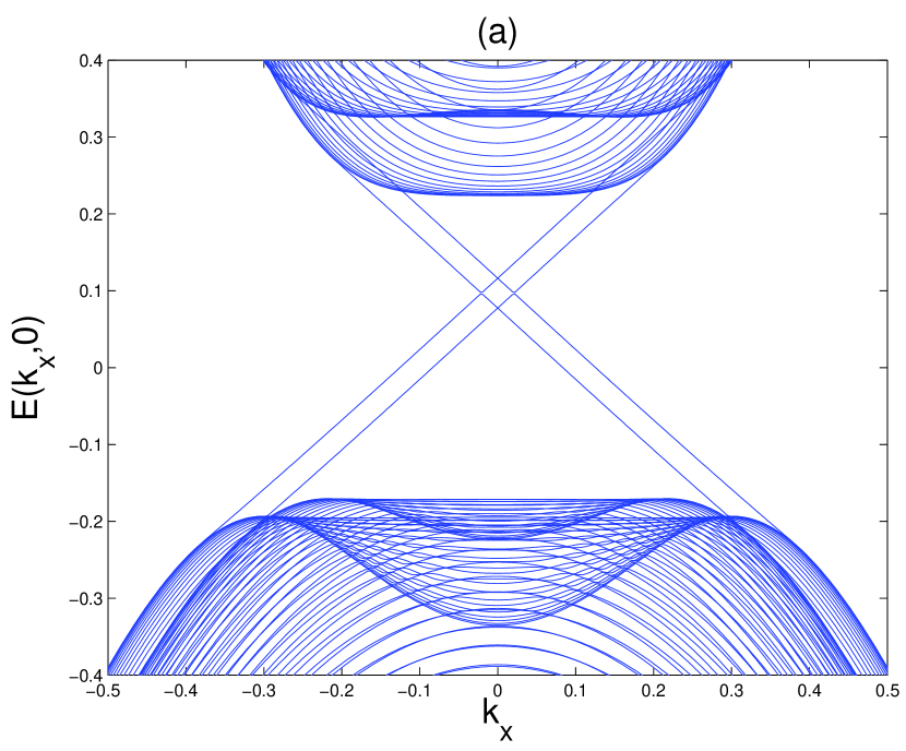
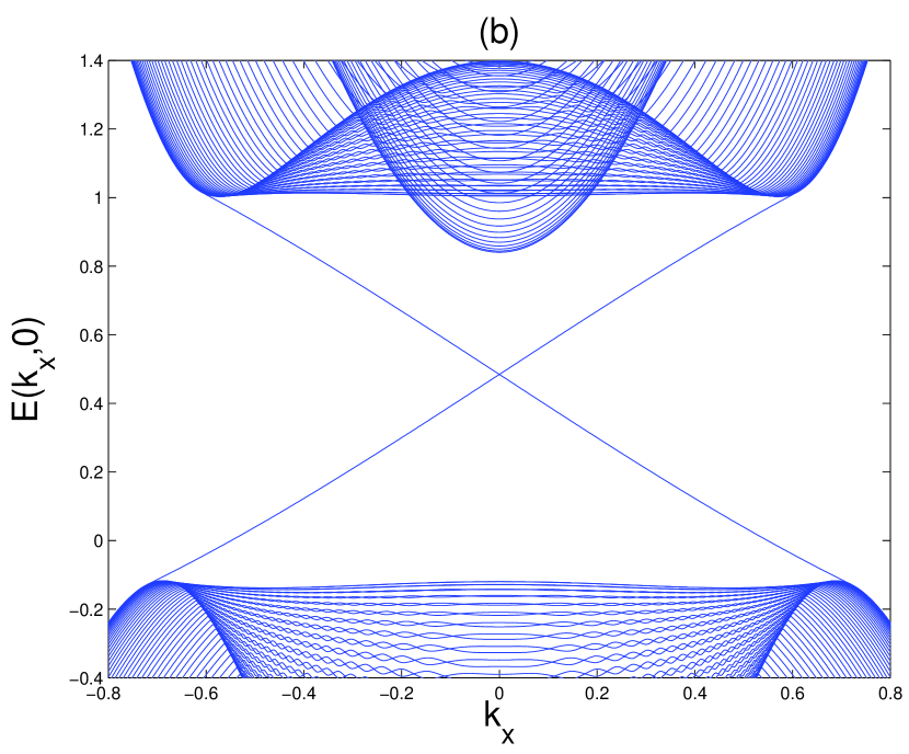
Figure 15: Numerical dispersions of bulk and surface states for model I with $V_{z}/M=0.2$ in (a) and (c) and $4.0$ in (b) and (d). In (a) and (b) $k_{z}=0$, and in (c) and (d) $k_{x}=0$. The other parameters are same as in figure 13

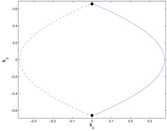
Figure 16: Surface Fermi arc for the set of parameters shown in figure 15 (b) and (d). The solid line shows the line of constant energy $E=0.144$ eV for the states at the $y=0$ surface, the dashed line for the opposite surface at $y=L$. The black dots at $(k_{x},k_{z})=(0,\pm 0.66)$ are the projections of the Weyl nodes onto the surface Brillouin zone. The Fermi arcs end there.

7.2 Model I with boundary perpendicular to the $z$-direction

In this case we find approximate surface state dispersions for small momenta $k_{x}$ and $k_{y}$ of the form

$$E_{\pm}(\mathbf{k})=C+Mt_{1}+2(D_{2}-B_{2}t_{1})(2-\cos k_{x}-\cos k_{y})$$ (111)

$$\pm\sqrt{V_{z}^{2}+(V_{x}+2\sqrt{1-t_{1}^{2}}A_{2}\sin k_{x})^{2}+(V_{y}+2\sqrt{1-t_{1}^{2}}A_{2}\sin^{2}k_{y})^{2}},$$

where $t_{1}=D_{1}/B_{1}$. Here, the $z$-component of the exchange field opens a gap in the Dirac dispersion, while both $x$- and $y$-components lead to a shift of the Dirac cone, leaving it intact. In this geometry there appear no Fermi arcs at the surface, as in the corresponding particle-hole symmetric case. This can be understood from the fact that both Weyl nodes sit on the $k_{z}$-axis. For that reason their projections onto a $k_{z}=$ const. plane fall on top of each other and the Fermi arc shrinks to zero. It is interesting to see that the physics of the Weyl semimetal state cannot be observed on a $z$-surface due to the structure of the Weyl state here. Experimentally one needs to look at the side surfaces or at a surface having a finite angle with the $z$-surface to observe the Fermi arc.

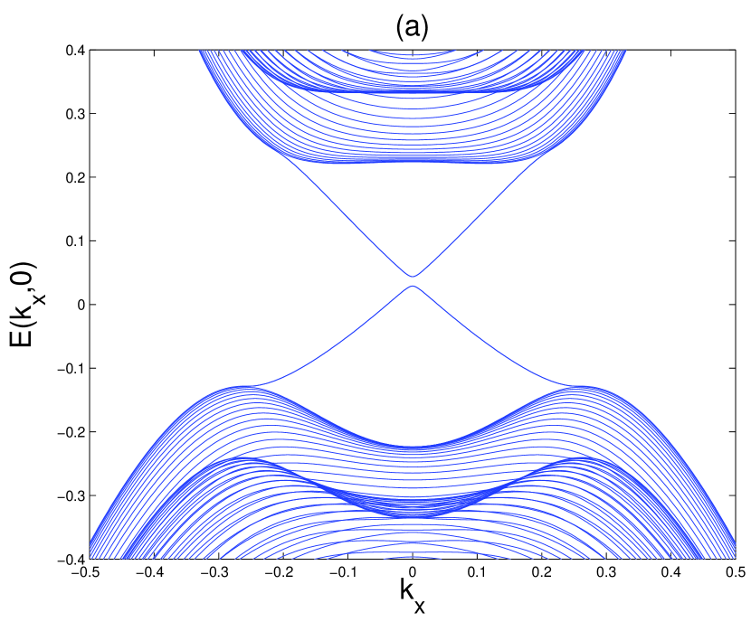
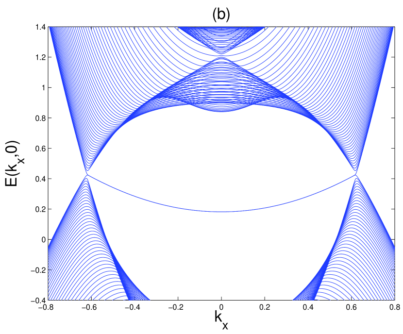
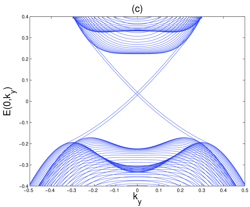
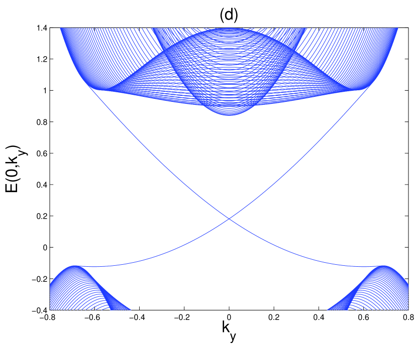
Figure 17: Numerical dispersions of bulk and surface states for model II with $V_{x}/M=0.2$ for (a) and (c) and $4.0$ for (b) and (d). In (a) and (b) $k_{y}=0$, and in (c) and (d) $k_{x}=0$. The other parameters are same as in figure 13

7.3 Model II with boundary perpendicular to the $z$-direction

In the absence of an exchange field the surface state dispersions are given by

$$E_{\pm}(\mathbf{k}) =C+Mt_{1}+2(D_{2}-B_{2}t_{1})(2-\cos k_{x}-\cos k_{y})$$ (112)

$$\pm\sqrt{1-t_{1}^{2}}2A_{2}\sqrt{\sin^{2}k_{x}+\sin^{2}k_{y}},$$

where $t_{1}=D_{1}/B_{1}\approx 0.13$. If $t_{1}>1$ surface states do not exist.

When the exchange field points into $x$-direction we find the following surface state dispersions

$$E_{\pm}(\mathbf{k}) =C+Mt_{1}+(D_{2}-B_{2}t_{1})(2-\cos k_{x}-\cos k_{y})$$

$$\pm\sqrt{4\beta^{2}_{6}(V_{x})\left(1-t_{1}^{2}\right)A_{2}^{2}\sin^{2}k_{x}+(t_{1}V_{x}-2\sqrt{1-t_{2}^{2}}A_{2}\sin k_{y})^{2}}.$$

where $\beta_{6}$ is given by

$$\beta_{6}(V_{x})=\frac{4A_{2}^{2}\sqrt{\tilde{m}_{0}^{2}-V_{x}^{2}-\frac{1}{1-t_{1}^{2}}\left(t_{1}^{2}A_{2}^{2}\sin^{2}k_{y}+4V_{x}t_{1}A_{2}\sqrt{1-t_{1}^{2}}\sin k_{x}\right)}}{4A_{2}^{2}\tilde{m}_{0}^{2}+4B_{2}V_{x}t_{1}A_{2}\sqrt{1-t_{1}^{2}}\sin k_{y}+B_{2}V_{x}^{2}+t_{1}^{2}B_{2}\left(4A_{2}^{2}\sin^{2}k_{y}-V_{x}^{2}\right)}$$ (114)

with $\tilde{m}_{0}=M-2B_{2}\left(1-\cos k_{x}\right)-2B_{2}\left(1-\cos k_{y}\right)$. From this dispersion we see that the Dirac cone remains ungapped for an exchange field in $x$-direction and is shifted in $k_{y}$ direction. Corresponding numerical results are shown in Fig. 17 (a) and (c) confirming this behavior. In Fig. 17 (b) and (d) we show results for $V_{x}>M$. Here, we see that again the corresponding one-dimensional flat band discussed in section 6.1 becomes dispersive now due to the broken particle-hole symmetry. Again, this system remains a Weyl semimetal, however. As pointed out in appendix I, in model II the Weyl nodes follow the direction of the exchange field and sit on the $k_{x}$-axis in the present case. The projections of the two Weyl nodes onto the surface Brillouin zone for $V_{z}=4M$ are found at $(k_{x},k_{y})=(\pm 0.623,0)$ in Fig. 17 (d). These are the points, where the surface band ends. Similarly as in Fig. 16 the lines of constant energy $E=0.421$ eV become curved and open Fermi arcs (not shown).

When the exchange field points into $z$-direction we find the following surface state dispersions

$$E_{\pm}(\mathbf{k}) =C+Mt_{1}+2(D_{2}-B_{2}t_{1})(2-\cos k_{x}-\cos k_{y})$$ (115)

$$\pm\sqrt{V_{z}^{2}+(1-t_{1}^{2})4A_{2}^{2}\left(\sin^{2}(k_{x})+\sin^{2}(k_{y})\right)}.$$

Thus, the application of an exchange field perpendicular to the surface leads to a gap in the Dirac dispersion. When $V_{z}$ is increased beyond $V_{cr}$ no flat band appears. This can be understood from the fact that in model II the Weyl nodes follow the field direction. Thus, for fields perpendicular to the surface their projections onto the surface Brillouin zone fall on top of each other and the Fermi arc disappears.

8 Summary and Conclusions

We have studied the modification of the surface states of a three dimensional topological insulator by a ferromagnetic exchange field using the two models that are presently discussed for topological insulators.

For model I, which is appropriate for the Bi₂Se₃ class of layered materials the surface states on a side surface behave qualitatively different than the ones on the top or bottom surface. For exchange fields smaller than the bulk gap the velocity of the Dirac cone can be tuned down to smaller values in an anisotropic way depending on the direction of the exchange field. For exchange fields larger than a critical value of the order of the bulk gap the system becomes a topologically nontrivial semimetal. We have shown that in a particle-hole symmetric system the Fermi surface of this semimetal is a line in momentum space, if the exchange field is directed within the $xy$-plane. In this case a two-dimensional flat band appears at a side surface. If the exchange field possesses a finite component in $z$-direction, there exist only single points in the Brillouin zone, where the bulk gap vanishes. We have shown that in this general case the system becomes a Weyl semimetal. Associated with this peculiar state of matter we find Fermi arcs at the side surfaces and one-dimensional flat bands.

If particle-hole symmetry is not obeyed, the flat bands become dispersive, but remain well separated from the bulk bands. The Weyl semimetallic phase and the existence of a surface Fermi arc is preserved also under broken particle-hole symmetry.

In model II, which is more isotropic than model I, the behavior on the top and side surfaces is qualitatively the same. For small exchange fields, it is again possible to tune the velocity of the Dirac cone by the exchange field anisotropically. For exchange fields larger than a critical value of the order of the bulk gap model II always enters a Weyl semimetal state. Associated with this we also find Fermi arcs and one-dimensional surface flat bands in this case. However, in model II there is no case in which a two-dimensional surface flat band appears.

If particle-hole symmetry is not obeyed, the flat bands become again dispersive. The Weyl semimetallic phase and the existence of a surface Fermi arc again is preserved under broken particle-hole symmetry.

The Weyl nodes in model I sit on the $k_{z}$ axis, while they move with the direction of the exchange field in model II. As a consequence, in model I the Fermi arcs and flat bands do not appear on the top and bottom surfaces, while in model II this is possible.

We have shown that the appearence of flat bands in our particle-hole symmetric cases could always be classified by topological invariants that have recently been given by Matsuura et al [51]. The invariants are related to different chiral symmetries in the different cases.

Surface flat bands have been proposed in systems like graphene, superfluid ³He, or unconventional superconductors before. However, in these systems cryogenic temperatures are required to observe the flat bands. In the materials discussed here, the energy scale is set by the bulk gap, which is of the order of 0.3 eV in Bi₂Se₃. Thus, flat bands could be observed already at room temperature. The fact that one can turn on or off a surface flat band by rotation of the magnetization of a ferromagnet makes the present system particularly interesting for applications in spintronics.

Appendix I

In this appendix we derive the ranges of the exchange field under which model I and II become semimetallic, i.e. the gap vanishes. It is only in the semimetallic phase that the system possesses surface flat bands. In particular it is of interest to know the critical value of the exchange field that is necessary to drive the system from the insulating into the semimetallic phase.

For model I we start from the bulk bandstructure of the four bands given in Eq. (2). We omit the diagonal term $\epsilon_{0}(\mathbf{k})\mathbb{I}_{4\times 4}$ in the Hamiltonian as it just shifts the four bands by $\epsilon_{0}(\mathbf{k})$ and thus does not affect the direct gap of the system. For large values of $D_{1}$ and $D_{2}$ this term can lead to an indirect gap, however.

As is clear from the symmetric spectrum Eq. (2) the gap closes when there exist momenta ${\mathbf{k}}$ for which $E_{i}^{I}({\mathbf{k}})$ becomes zero. To determine those momenta it is beneficial to write the exchange field in spherical coordinates, i.e. $V_{x}=V\cos\varphi\cos\vartheta$, $V_{y}=V\sin\varphi\cos\vartheta$, and $V_{z}=V\sin\vartheta$. If one exploits the fact that

$$\left(m_{1}\sin\varphi\cos\vartheta-m_{2}\cos\varphi\cos\vartheta\right)^{2}+\left(m_{1}\cos\varphi\cos\vartheta+m_{2}\sin\varphi\cos\vartheta\right)^{2}$$

$$=\left(m_{1}^{2}+m_{2}^{2}\right)\left(1-\sin^{2}\vartheta\right)\,,$$

Eq. (2) can be written in the form

$$E_{i}^{I}(\mathbf{k}) =\pm\Big{\{}\left(m_{1}\sin\varphi\cos\vartheta-m_{2}\cos\varphi\cos\vartheta\right)^{2}+\sin^{2}\vartheta\left(m_{1}^{2}+m_{2}^{2}\right)+$$ (116)

$$+\left(V\pm\sqrt{m_{0}^{2}+m_{3}^{2}+\left(m_{1}\cos\varphi\cos\vartheta+m_{2}\sin\varphi\cos\vartheta\right)^{2}}\right)^{2}\Big{\}}^{1/2}$$

This expression can become zero only, if all squared expressions below the square-root become zero simultaneously. For $V_{z}\neq 0$ this means $m_{1}=m_{2}=0$ and $V^{2}=m_{0}^{2}+m_{3}^{2}$. For a given value of $V$ the gap will close only in a single pair of bands. From $m_{1}=m_{2}=0$ it follows that $k_{x}=0$ or $\pi$ and $k_{y}=0$ or $\pi$. The equation $V^{2}=m_{0}^{2}+m_{3}^{2}$ can then only be fulfilled for selected values of $k_{z}$. Thus the system will have single Fermi points, when a solution exists. For the special case $\vartheta=0$, i.e. when the exchange field lies within the $x$-$y$-plane, there are just two equations to be fulfilled, i.e. $m_{1}\sin\varphi=m_{2}\cos\varphi$ and $V^{2}=m_{0}^{2}+m_{3}^{2}+\left(m_{1}\cos\varphi+m_{2}\sin\varphi\right)^{2}$. In this case the Fermi surface will be a line in momentum space.

To determine the ranges of the exchange field for which these solutions exist, we determine the minimum and maximum value of $m_{0}^{2}+m_{3}^{2}$. Let us set $c=\cos k_{z}$. Then we have to minimize the function

$$f(c)=\left[M^{\prime}-2B_{1}\left(1-c\right)\right]^{2}+4A_{1}^{2}\left(1-c^{2}\right)$$ (117)

in the interval $c\in\left[-1,1\right]$. Here, we have set

$$M^{\prime} =\left\{\begin{array}[]{cl}M&\mbox{for}\,k_{x}=k_{y}=0\\ M-4B_{2}&\mbox{for}\,(k_{x}=0\,\mbox{and}\,k_{y}=\pi)\,\,\mbox{or}\,\,(k_{x}=\pi\,\mbox{and}\,k_{y}=0)\\ M-8B_{2}&\mbox{for}\,k_{x}=k_{y}=\pi\end{array}\right.$$ (121)

The function $f(c)$ is quadratic in $c$, so there can only be a single extremum within $c\in\left[-1,1\right]$ or the extremum will be on the boundaries $c=\pm 1$. On the boundaries we have

$$f(c=1) ={M^{\prime}}^{2}\quad\mbox{and}\quad f(c=-1)=\left(4B_{1}-M^{\prime}\right)^{2}$$

As we assume $B_{1}>M>0$ and $B_{2}>M>0$, we have $f(c=-1)>f(c=1)$. To determine a possible extremum inside the interval $c\in\left[-1,1\right]$ we take the derivative of $f(c)$ yielding

$$\frac{df}{dc} =4M^{\prime}B_{1}-8B_{1}^{2}+\left(8B_{1}^{2}-8A_{1}^{2}\right)c$$

This becomes zero, if

$$c=c_{min}=\frac{B_{1}\left(2B_{1}-M^{\prime}\right)}{2\left(B_{1}^{2}-A_{1}^{2}\right)}$$ (122)

The second derivative of $f(c)$ is

$$\frac{d^{2}f}{dc^{2}}=8\left(B_{1}^{2}-A_{1}^{2}\right)\,.$$

As we assume $B_{1}>A_{1}$, this is positive. We thus find that there exists a minimum inside the interval $c\in\left[-1,1\right]$, if

$$\left|\frac{B_{1}\left(2B_{1}-M^{\prime}\right)}{2\left(B_{1}^{2}-A_{1}^{2}\right)}\right|\leq 1$$

which is equivalent to the condition

$$M^{\prime}B_{1}\geq 2A_{1}^{2}$$

This condition can only be fulfilled for positive $M^{\prime}$, i.e. only for $k_{x}=k_{y}=0$. Thus, in the case $MB_{1}\geq 2A_{1}^{2}$, the minimum for the exchange field can be found by introducing Eq. (122) into Eq. (117). After some algebra one finds

$$f(c_{min})=\frac{A_{1}^{2}\left(4B_{1}M-M^{2}-4A_{1}^{2}\right)}{B_{1}^{2}-A_{1}^{2}}$$

Thus we find that the minimum critical value $V_{cr}$ for the magnitude of the exchange field, which is necessary to bring the system into the semimetallic phase, is given by

$$V_{cr}=\left\{\begin{array}[]{cl}M&\mbox{for}\,MB_{1}<2A_{1}^{2}\\ A_{1}\sqrt{\frac{4B_{1}M-M^{2}-4A_{1}^{2}}{B_{1}^{2}-A_{1}^{2}}}&\mbox{for}\,MB_{1}\geq 2A_{1}^{2}\end{array}\right.$$ (123)

In total we find the following three ranges for the magnitude of the exchange field, in which the system becomes semimetallic: $\left[V_{cr},4B_{1}-M\right]$, $\left[4B_{2}-M,4B_{1}+4B_{2}-M\right]$, and $\left[8B_{2}-M,4B_{1}+8B_{2}-M\right]$. For $B_{2}\geq B_{1}$ these ranges overlap, while for $B_{2}<B_{1}$ they are separate. As $B_{1}$ and $B_{2}$ are usually of the order of one to several eV, we do not expect that large enough exchange fields can be applied in practice to actually observe these different ranges. However, the minimum critical field $V_{cr}$, which is of the order of $M$ or less, is within experimental reach.

The position of the Fermi points is found from the quadratic equation

$$V^{2}=f(c)$$ (124)

For $V\in\left[V_{cr},4B_{1}-M\right]$ the Fermi points sit on the $k_{z}$-axis ($k_{x}=k_{y}=0$). Their positions are given by

$$c_{1/2}=c_{min}\pm\frac{\sqrt{A_{1}^{2}\left(M^{2}-4MB_{1}+4A_{1}^{2}\right)+V^{2}\left(B_{1}^{2}-A_{1}^{2}\right)}}{2\left(B_{1}^{2}-A_{1}^{2}\right)}$$ (125)

For the case $MB_{1}\geq 2A_{1}^{2}$ and $V<M$ both solutions are within the interval $c\in\left[-1,1\right]$ and we thus have a total of four Fermi points at the positions $k_{z,1/2}=\pm\arccos c_{1}$ and $k_{z,3/4}=\pm\arccos c_{2}$. In the other case $MB_{1}<2A_{1}^{2}$ only solution $c_{2}$ with the minus sign in Eq.(125) is within $\left[-1,1\right]$ and we have just two Fermi points at $k_{z,1/2}=\pm\arccos c_{2}$.

For the special case $V_{z}=0$ the minimum value of the exchange field to bring the system into the semimetallic state remains the same. In this case the function

$$V^{2}=m_{0}^{2}+m_{3}^{2}+\left(m_{1}\cos\varphi+m_{2}\sin\varphi\right)^{2}$$

has to be minimized. However, as the minimum of $m_{0}^{2}+m_{3}^{2}$ occurs at $k_{x}=k_{y}=0$ and $m_{1}=m_{2}=0$ there, the minimum of $V$ remains the same value $V_{cr}$ Eq. (123). Also, for $V>V_{cr}$ the two (or four) points determined above still lie on the Fermi surface. However, as pointed out above, the Fermi surface becomes a line (or two lines) now, which approximately run within the plane perpendicular to the exchange field (The precise condition is that the vector $(m_{1},m_{2})^{T}=2A_{2}(\sin k_{x},\sin k_{y})^{T}$ should be perpendicular to the exchange field $(V_{x},V_{y})$.)

Let us next look at model II. We again write the exchange field in spherical coordinates, i.e. $V_{x}=V\cos\varphi\cos\vartheta$, $V_{y}=V\sin\varphi\cos\vartheta$, and $V_{z}=V\sin\vartheta$. This time Eq. (3) can be written in the form

$$E_{i}^{II}(\mathbf{k}) =\pm\Big{\{}\left(m_{1}\sin\varphi-m_{2}\cos\varphi\right)^{2}+\left(m_{1}\cos\varphi\sin\vartheta+m_{2}\sin\varphi\sin\vartheta-m_{3}\cos\vartheta\right)^{2}+$$ (126)

$$+\left(V\pm\sqrt{m_{0}^{2}+\left(m_{1}\cos\varphi\cos\vartheta+m_{2}\sin\varphi\cos\vartheta+m_{3}\sin\vartheta\right)^{2}}\right)^{2}\Big{\}}^{1/2}$$

This expression can become zero only, if all three squared expressions below the square-root vanish simultaneously. This means that the system will have Fermi points, when a zero energy solution exists. The first two expression become zero, if the vector $(m_{1},m_{2},m_{3})$ is parallel to $(\cos\varphi\cos\vartheta,\sin\varphi\cos\vartheta,\sin\vartheta)$, i.e. parallel to the exchange field. The third equation can then be written as

$$V^{2} =m_{0}^{2}+m_{1}^{1}+m_{2}^{2}+m_{3}^{2}$$

It is clear that the minimum critical value $V_{cr}$ for the magnitude of the exchange field, which is necessary to bring the system into the semimetallic phase fulfils $V_{cr}\leq M$, because a zero energy state can always be found for $k_{x}=k_{y}=k_{z}=0$ and $V=M$. A general expression for $V_{cr}$ can in principle be obtained analytically for exchange field in any direction. However, the expressions become quite complicated. Therefore, here we focus on the two cases that the exchange field points either in $x$-direction or in $z$-direction.

For exchange field in $x$-direction we have $m_{2}=m_{3}=0$. The minimum can thus be found on the $k_{x}$-axis by minimizing the function $f(c)$ Eq. (117) with $c=\cos k_{x}$ and $B_{1}$ and $A_{1}$ being replaced by $B_{2}$ and $A_{2}$. Following the same calculation as for model I we then find for the critical value $V_{cr,x}$ in this case:

$$V_{cr,x}=\left\{\begin{array}[]{cl}M&\mbox{for}\,MB_{2}<2A_{2}^{2}\\ A_{2}\sqrt{\frac{4B_{2}M-M^{2}-4A_{2}^{2}}{B_{2}^{2}-A_{2}^{2}}}&\mbox{for}\,MB_{2}\geq 2A_{2}^{2}\end{array}\right.$$ (127)

Analogously to model I, for $V>V_{cr,x}$ we have either two or four Fermi points lying on the $k_{x}$-axis. Their positions are found from

$$c_{1/2}=c_{min}\pm\frac{\sqrt{A_{2}^{2}\left(M^{2}-4MB_{2}+4A_{2}^{2}\right)+V^{2}\left(B_{2}^{2}-A_{2}^{2}\right)}}{2\left(B_{2}^{2}-A_{2}^{2}\right)}$$ (128)

For exchange field in $z$-direction we have $m_{1}=m_{2}=0$. The minimum can thus be found on the $k_{z}$-axis by minimizing the same function $f(c)$ Eq. (117) as for model I. We thus find for the critical value $V_{cr,z}$ in this case:

$$V_{cr,z}=\left\{\begin{array}[]{cl}M&\mbox{for}\,MB_{1}<2A_{1}^{2}\\ A_{1}\sqrt{\frac{4B_{1}M-M^{2}-4A_{1}^{2}}{B_{1}^{2}-A_{1}^{2}}}&\mbox{for}\,MB_{1}\geq 2A_{1}^{2}\end{array}\right.$$ (129)

From this expression we see that for model II in general the critical value $V_{cr}$ depends on the direction of the exchange field, in contrast to model I, where it was isotropic. The position of the Fermi points in this case is given by Eq. (125) for $V>V_{cr,z}$. Again, one sees that the position of the Fermi points in model II varies with the direction of the exchange field, in contrast to model I.

Appendix II

During the course of this work we repeatedly encounter the situation that the Hamiltonian can be written in the following form:

$$H({\bf k}) =H_{0}({\bf k})+H^{\prime}({\bf k})$$

$$H^{\prime}({\bf k}) =f({\bf k})A+g({\bf k})B$$

where $f(\bf k)$ and $g(\bf k)$ are complex functions. $A$ is a momentum independent operator that commutes with $H_{0}(\bf k)$, while $B$ anticommutes with $H_{0}(\bf k)$. We would like to determine the eigenstates and eigenvalues of $H(\bf k)$ from the known eigenstates and eigenvalues of $H_{0}(\bf k)$. Due to the symmetries and the $4\times 4$ structure for each momentum $\bf k$ $H_{0}(\bf k)$ possesses at most two degenerate states with energy $E_{0}(\bf k)$ and two degenerate states with energy $-E_{0}(\bf k)$.

Let $\left|1\right\rangle$ be an eigenstate of $H_{0}$ with energy $E$. Then $A\left|1\right\rangle$ will also be an eigenstate of $H_{0}$ with energy $E$ and $B\left|1\right\rangle$ will be an eigenstate of $H_{0}$ with energy $-E$. Thus,

$$A\left|1\right\rangle={\sum_{j}}^{+}a_{j}\left|j\right\rangle$$ (130)

where the sum goes over all the eigenstates of $H_{0}$ with energy E, and

$$B\left|1\right\rangle={\sum_{n}}^{-}b_{n}\left|n\right\rangle$$ (131)

where the sum goes over all the eigenstates of $H_{0}$ with energy -E. In total we have

$$H^{\prime}\left|1\right\rangle=f({\bf k}){\sum_{j}}^{+}a_{j}\left|j\right\rangle+g({\bf k}){\sum_{n}}^{-}b_{n}\left|n\right\rangle$$ (132)

Thus, $H^{\prime}$ can only couple the eigenstates of $H_{0}$ with energies $E$ and $-E$. This means that the total Hamiltonian $H$ in the basis of the eigenstates of $H_{0}$ is reduced to (at most) $4\times 4$ blocks. The problem of finding the eigenstates and eigenvalues of $H(\bf k)$ thus reduces to $4\times 4$ matrices within the $\pm E$ spaces of $H_{0}$.

In the cases discussed in this manuscript we are interested in surface states localized on a single side of the system. We construct $H_{0}$ in such a way that its surface states have zero energy. We then have to diagonalize $H^{\prime}$ in the $E=0$ subspace of $H_{0}$. The eigenvalues and eigenstates of $H^{\prime}$ in this subspace are then the surface states of $H$ and their energies that we look for. As the number of localized states at one surface of the system is equal to the number of localized states at the oppsite surface due to parity symmetry, we are only left to solve a $2\times 2$ problem. So the general procedure, which we take in this manuscript, is to first determine the zero energy eigenstates of $H_{0}$ (if they exist) and then determine the eigenvalues and eigenstates of $H^{\prime}$ in this subspace.

Appendix III

In this appendix we derive an analytical condition for the existence of the two-dimensional flat band based on the winding number

$$w(k_{x},k_{z})=\frac{1}{2\pi}\textrm{Im}\int_{-\pi}^{\pi}\,dk_{y}\,\left(\textrm{det}D(\mathbf{k})\right)^{-1}\partial_{k_{y}}\textrm{det}D(\mathbf{k}).$$ (133)

To evaluate this expression analytically it is useful to employ the residue theorem in the following way [67]: for given $k_{x}$ and $k_{z}$ the quantity

$$\gamma(\mathbf{k})=\textrm{det}D(\mathbf{k})=m_{0}^{2}+m_{1}^{2}+m_{2}^{2}+m_{3}^{2}-V_{x}^{2}-V_{y}^{2}+2im_{1}V_{y}-2im_{2}V_{x}$$ (134)

for $k_{y}\in[-\pi,\pi]$ defines a closed path in the complex plane. Therefore, by transforming $z=\textrm{det}D(\mathbf{k})$ the winding number can be expressed as the integral

$$w(k_{x},k_{z})=\frac{1}{2\pi}\textrm{Im}\oint_{\gamma}\,\frac{dz}{z}=I(\gamma,0).$$ (135)

where $I(\gamma,0)$ is the winding number of the curve $\gamma$ around the origin. Thus, if the curve does not enclose the origin, the winding number becomes zero and no zero energy surface state exists. Now, the path $\gamma$ crosses the real axis, when $\textrm{Im}\;\textrm{det}D(\mathbf{k})=0$. This happens, when

$$m_{1}V_{y}=m_{2}V_{x}\qquad\Longleftrightarrow\qquad\sin k_{y}=\frac{V_{y}}{V_{x}}\sin k_{x}$$ (136)

For a given $k_{x}$ this equation has two solutions $k_{y,1}$ and $k_{y,2}=\pi-k_{y,1}$, if $\frac{V_{y}}{V_{x}}\sin k_{x}\in(-1,1)$. The path encloses the origin only, if these two crossings possess different sign of the real part, i.e. the criterion for the existence of the flat band becomes

$$0>\gamma(k_{x},k_{y,1},k_{z})\;\gamma(k_{x},k_{y,2},k_{z}).$$ (137)

The boundary of the flat band in $k_{x}$-$k_{z}$-space is then given by the criterion

$$0=\gamma(k_{x},k_{y,1},k_{z})\;\gamma(k_{x},k_{y,2},k_{z}).$$ (138)

Now, as on the Fermi surface we have $\textrm{det}D(\mathbf{k})=0$, it follows that the boundary of the flat band is just the projection of the (one-dimensional) Fermi surface onto the $k_{x}$-$k_{z}$-plane.

In the general case the analytical expression Eq. (137) becomes quite complicated. However, the expression can be simplified in the case $V_{y}=0$, as then $k_{y,1}=0$ and $k_{y,2}=\pi$. Then we have

$$\gamma(k_{x},0,k_{z}) =\tilde{m}_{0}(\mathbf{k})^{2}+4A_{2}^{2}\sin^{2}k_{x}+4A_{1}^{2}\sin^{2}k_{z}-V_{x}^{2}$$ (139)

$$\gamma(k_{x},\pi,k_{z}) =\left[\tilde{m}_{0}(\mathbf{k})-4B_{2}\right]^{2}+4A_{2}^{2}\sin^{2}k_{x}+4A_{1}^{2}\sin^{2}k_{z}-V_{x}^{2}$$

where $\tilde{m}_{0}(\mathbf{k})=M-2B_{2}(1-\cos k_{x})-2B_{1}(1-\cos k_{z})$. If we look at $k_{x}=k_{z}=0$, we see that $\gamma(0,0,0)$ becomes negative, when $|V_{x}|>M$. $\gamma(0,\pi,0)$ becomes negative, when $|V_{x}|>4B_{2}-M$. As we assume $B_{2}>M$ here, $\gamma(0,\pi,0)$ will change sign only at much larger fields $|V_{x}|$. Therefore, a flat band will be present in the vicinity of $k_{x}=k_{z}=0$ for $4B_{2}-M>|V_{x}|>M$.

References

References

- [1] B. A. Bernevig, T. L. Hughes, and S.-C. Zhang, Science 314, 1757 (2006).
- [2] L. Fu, C. L. Kane and E. J. Mele, Phys. Rev. Lett. 98, 106803 (2007).
- [3] M. König, S. Wiedmann, C. Brüne, A. Roth, H. Buhmann, L.W. Molenkamp, X.-L. Qi, and S.-C. Zhang, Science 318, 766 (2007).
- [4] D. Hsieh, D. Qian, L. Wray, Y. Xia, Y. Hor, R. J. Cava, and M. Z. Hasan, Nature (London) 452, 970 (2008).
- [5] Y. L. Chen, J G. Analytis, J.-H. Chu, Z. K. Liu, S.-K. Mo, X. L. Qi, H. J. Zhang, D. H. Lu, X. Dai, Z. Fang, S. C. Zhang, I. R. Fisher, Z. Hussain, and Z.-X. Shen, Science 325, 178 (2009).
- [6] Y. Xia, D. Qian, D. Hsieh, L. Wray, A. Pal, H. Lin, A. Bansil, D. Grauer, Y. S. Hor, R. J. Cava, and M. Z. Hasan, Nature Phys. 5, 398 (2009).
- [7] D. Hsieh, Y. Xia, D. Qian, L. Wray, F. Meier, J. H. Dil, J. Osterwalder, L. Patthey, A. V. Fedorov, H. Lin, A. Bansil, D. Grauer, Y. S. Hor, R. J. Cava, and M. Z. Hasan, Phys. Rev. Lett. 103, 146401 (2009).
- [8] K. Kuroda et al, Phys. Rev. Lett. 108, 206803 (2012).
- [9] S. Chadov, X. Qi, J. Kübler, G. H. Fecher, C. Felser, and S. C. Zhang, Nature Mat. 9, 541 (2010).
- [10] H. Lin, L. A. Wray, Y. Xia, S. Xu, S. Jia, R. J. Cava, A. Bansil, and M. Z. Hasan, Nature Mat. 9, 546 (2010).
- [11] M. Z. Hasan and C. L. Kane, Rev. Mod. Phys. 82, 3045 (2010).
- [12] Y. Ando, J. Phys. Soc. Japan 82, 102001 (2013).
- [13] I. Garate and M. Franz, Phys. Rev. Lett. 104, 146802 (2010).
- [14] T. Yokoyama , Y. Tanaka, and N. Nagaosa, Phys. Rev. B 81, 121401(R) (2010).
- [15] R. Yu, W. Zhang, H.-J. Zhang, S.-C. Zhang, X. Dai, and Z. Fang, Science 329, 61 (2010).
- [16] Y. L. Chen et al, Science 329, 659 (2010).
- [17] Y. S. Hor, et al, Phys. Rev. B 81, 195203 (2010).
- [18] P. Wei, F. Katmis, B. A. Assaf, H. Steinberg, P. Jarillo-Herrero, D. Heiman, and J. S. Moodera, Phys. Rev. Lett. 110, 186807 (2013).
- [19] A.M. Black-Schaffer and J. Linder, Phys. Rev. B 84, 180509(R) (2011).
- [20] R. L. Chu, J. Shi, and S.-Q. Shen, Phys. Rev. B 84, 085312 (2011).
- [21] J. Honolka et al., Phys. Rev. Lett. 108, 256811 (2012).
- [22] M. R. Scholz, J. Sánchez-Barriga, D. Marchenko, A. Varykhalov, A. Volykhov, L.V. Yashina, and O. Rader, Phys. Rev. Lett. 108, 256810 (2012).
- [23] A. M. Lunde and G. Platero, Phys. Rev. B 88, 115411 (2013).
- [24] T. Paananen and T. Dahm, Phys. Rev. B 87, 195447 (2013).
- [25] K. Nakada, M. Fujita, G. Dresselhaus and M. S. Dresselhaus, Phys. Rev. B 54, 17954 (1996).
- [26] T. Mizushima, M. Sato, and K. Machida, Phys. Rev. Lett. 109, 165301 (2012).
- [27] M. A. Silaev and G. E. Volovik, Phys. Rev. B 86, 214511 (2012).
- [28] A. P. Schnyder, C. Timm, and P. M. R. Brydon, Phys. Rev. Lett. 111, 077001 (2013).
- [29] P. M. R. Brydon, C. Timm, and A. P. Schnyder, New J. Phys. 15, 045019 (2013).
- [30] C. L. M. Wong, J. Liu, K. T. Law, and P. A. Lee, Phys. Rev. B 88, 060504 (2013).
- [31] J. D. Sau and S. Tewari, Phys. Rev. B 86, 104509 (2012).
- [32] A. Lau and C. Timm, arXiv:1305.1770 (2013).
- [33] C.-R. Hu, Phys. Rev. Lett. 72, 1526 (1994).
- [34] Y. Tanaka and S. Kashiwaya, Phys. Rev. Lett. 74, 3451 (1995).
- [35] S. Kashiwaya and Y. Tanaka, Rep. Prog. Phys. 63, 1641 (2000).
- [36] G. E. Volovik, JETP Lett. 93, 66 (2011).
- [37] T. T. Heikkilä, N. B. Kopnin, and G. E. Volovik, JETP Lett. 94, 233 (2011); G. E. Volovik, J. Supercond. Nov. Magn. 26, 2887 (2013).
- [38] S. Ryu and Y. Hatsugai, Phys. Rev. Lett. 89, 077002 (2002).
- [39] M. Sato, Phys. Rev. B 73, 214502 (2006).
- [40] M. Fogelström, D. Rainer, and J.A. Sauls, Phys. Rev. Lett. 79, 281 (1997).
- [41] H. Walter, W. Prusseit, R. Semerad, H. Kinder, W. Assmann, H. Huber, H. Burkhardt, D. Rainer, and J. A. Sauls, Phys. Rev. Lett. 80, 3598 (1998).
- [42] M. Aprili, E. Badica, and L. H. Greene, Phys. Rev. Lett. 83, 4630 (1999).
- [43] R. Krupke and G. Deutscher, Phys. Rev. Lett. 83, 4634 (1999).
- [44] B. Chesca, M. Seifried, T. Dahm, N. Schopohl, D. Koelle, R. Kleiner, A. Tsukada, Phys. Rev. B 71, 104504 (2005).
- [45] B. Chesca, D. Dönitz, T. Dahm, R. P. Huebener, D. Koelle, R. Kleiner, Ariando, H.-J. H. Smilde, H. Hilgenkamp, Phys. Rev. B 73, 014529 (2006).
- [46] C. Iniotakis, T. Dahm, and N. Schopohl, Phys. Rev. Lett. 100, 037002 (2008).
- [47] S. Graser, C. Iniotakis, T. Dahm, and N. Schopohl, Phys. Rev. Lett. 93, 247001 (2004).
- [48] Yu. S. Barash, M. S. Kalenkov, and J. Kurkijärvi, Phys. Rev. B 62, 6665 (2000).
- [49] A. Zare, T. Dahm, and N. Schopohl, Phys. Rev. Lett. 104, 237001 (2010).
- [50] A. P. Zhuravel, B. G. Ghamsari, C. Kurter, P. Jung, S. Remillard, J. Abrahams, A. V. Lukashenko, A. V. Ustinov, and S. M. Anlage, Phys. Rev. Lett. 110, 087002 (2013).
- [51] S. Matsuura, P.-Y. Chang, A. P. Schnyder, and S. Ryu, New J. Phys. 15, 065001 (2013).
- [52] X. Wan, A. M. Turner, A. Vishwanath, and S. Y. Savrasov, Phys. Rev. B 83, 205101 (2011).
- [53] L. Balents, Physics 4, 36 (2011).
- [54] A. A. Burkov and L. Balents, Phys. Rev. Lett. 107, 127205 (2011).
- [55] R. Li, J. Wang, X.-L. Qi, and S.-C. Zhang, Nature Phys. 6, 284 (2010).
- [56] H. Zhang, C.-X. Liu, X.-L. Qi, X. Dai, Z. Fang, and S.-C. Zhang, Nature Phys. 5, 438 (2009).
- [57] C.-X. Liu, X.-L. Qi, H. Zhang, X. Dai, Z. Fang, and S.-C. Zhang, Phys. Rev. B 82, 045122 (2010).
- [58] W.-Y. Shan, H.-Z. Lu, and S.-Q. Shen, New J. Phys. 12, 043048 (2010).
- [59] L. Hao and T. K. Lee, Phys. Rev. B 83, 134516 (2011).
- [60] P. G. Silvestrov, P. W. Brouwer, and E. G. Mishchenko, Phys. Rev. B 86, 075302 (2012).
- [61] A. P. Schnyder, S. Ryu, A. Furusaki and A.W.W. Ludwig, Phys. Rev. B 78, 195125 (2008).
- [62] S. Ryu, A. P. Schnyder, A. Furusaki and A. Ludwig, New J. Phys. 12, 065010 (2010).
- [63] A. Altland, B. D. Simons, and Z. R. Zirnbauer, Phys. Rep. 359, 283 (2002).
- [64] A. P. Schnyder and S. Ryu, Phys. Rev. B 84, 060504(R) (2011); P. M. R. Brydon, A.P. Schnyder, and C. Timm, Phys. Rev. B 84, 020501(R) (2011); A.P. Schnyder, P. M. R. Brydon, and C. Timm, Phys. Rev. B 85, 024522 (2012).
- [65] C. Brüne, A. Roth, H. Buhmann, E. M. Hankiewicz, L. W. Molenkamp, J. Maciejko, X.-L. Qi, and S.-C. Zhang, Nature Phys. 8, 485 (2012).
- [66] S. Murakami, New J. Phys. 9, 356 (2007).
- [67] H. Gerber, Bachelor thesis, Bielefeld University (2013).