Parallaxes for W49N and G048.60$+$0.02:
Distant Star Forming Regions in the Perseus Spiral Arm

Abstract

We report trigonometric parallax measurements of 22 GHz H₂O masers in two massive star-forming regions from VLBA observations as part of the BeSSeL Survey. The distances of $11.11^{+0.79}_{-0.69}$ kpc to W49N (G043.16$+$0.01) and $10.75^{+0.61}_{-0.55}$ kpc to G048.60$+$0.02 locate them in a distant section of the Perseus arm near the solar circle in the first Galactic quadrant. This allows us to locate accurately the inner portion of the Perseus arm for the first time. Combining the present results with sources measured in the outer portion of the arm in the second and third quadrants yields a global pitch angle of 9.5^∘ $\pm$ 1.3^∘ for the Perseus arm. We have found almost no H₂O maser sources in the Perseus arm for 50^∘ $<\ell<$ 80^∘, suggesting that this $\approx 6$ kpc section of the arm has little massive star formation activity.

1 INTRODUCTION

While the nature and even the number of spiral arms in the Milky Way is still debated, mounting evidence suggests that the Perseus arm is one of two major spiral arms (Drimmel, 2000; Benjamin et al., 2005; Churchwell et al., 2009). It may emerge from the far end of the bar and wrap through the inner Galaxy in the first quadrant (inner portion of the Perseus arm) and the outer Galaxy in the second and third quadrants (outer portion of the Perseus arm). Since the inner portion of the Perseus arm lies at a smaller Galactic radius and closer to the bar than the outer portion of the arm, one would expect it to be more prominent in molecular gas and star formation, yet very little is known about it owing to its great distance and its kinematic blending with nearer material in the inner Galaxy.

Recent improvements in radio astrometry with Very Long Baseline Interferometry (VLBI) techniques have yielded parallaxes and proper motions to star-forming regions in the Galaxy with accuracies of $\sim$ 10 $\mu$as and $\sim$ 0.1 mas yr^-1, respectively (e.g. Reid et al. 2009b; Honma et al. 2012). Parallax measurements for a reasonably dense sampling of sources in spiral arms will help us to fully trace the spiral structure of the Galaxy. To reach this goal, we are using the NRAO Very Long Baseline Array (VLBA) to conduct a key science project, the BeSSeL (Bar and Spiral Structure Legacy) Survey, to study the structure and kinematics of the Galaxy by measuring trigonometric parallaxes and proper motions for hundreds of 22 GHz H₂O and 6.7/12.2 GHz CH₃OH maser sources associated with massive star-forming regions.

In this paper, we present trigonometric parallax measurements of 22 GHz H₂O masers toward two high-mass star-forming regions, W49N (G043.16$+$0.01) and G048.60$+$0.02, in the inner portion of the Perseus arm.

2 OBSERVATIONS AND CALIBRATION PROCEDURES

Our observations of 22 GHz H₂O masers toward G043.16$+$0.01 and G048.60$+$0.02, together with several compact extragalactic radio sources, were carried out under VLBA program BR145B with 12 epochs spanning about one year. For these sources, the parallax signature in Declination was considerably smaller than for Right Ascension, and we scheduled the observations so as to maximize the Right Ascension parallax offsets as well as to minimize correlations among the parallax and proper motion parameters. The observations near each Right Ascension parallax peak were grouped as listed in Table 1. At each epoch, the observations consisted of four 0.5-hour “geodetic blocks” (used to calibrate and remove unmodeled atmospheric signal delays), with three 1.7-hour periods of phase-referenced observations inserted between the blocks. In the phase-referenced observations, we cycled between the target maser and several background sources, switching sources every 20 to 30 seconds. Table 2 lists the observed source positions, intensities, source separations, reference maser radial velocities and restoring beams. The typical on-source integration time per epoch for the maser source and each background source were 0.64 and 0.30 hour for G043.16$+$0.01, and 0.79 and 0.25 hour for G048.60$+$0.02, respectively.

Our general observing setup and calibration procedures are described in Reid et al. (2009a); here we discuss only aspects of the observations that are specific to the maser sources presented in this paper. We used four adjacent intermediate frequency (IF) bands with 16 MHz, each in both right and left circular polarization (RCP and LCP); the second band contained the maser signals, the center $V_{\rm LSR}$ is 10 and 26 km s^-1 for G043.16$+$0.01 and G048.60$+$0.02, respectively. The spectral-channel spacing was 31.25 kHz corresponding to 0.42 km s^-1 in velocity. We observed three International Celestial Reference Frame (ICRF) sources: 3C345 (J2253+1608), 3C454 (J1642+3948) and J1925+2106 (Ma et al., 1998), near the beginning, middle and end of the phase-referencing observations in order to monitor delay and electronic phase differences among the observing bands. The data correlation was performed with the DiFX software correlator (Deller et al., 2007) in Socorro, NM. The data reduction was conducted using the NRAO’s Astronomical Image Processing System ($\mathcal{AIPS}$) together with scripts written in ParselTongue (Kettenis et al., 2006). Since in our case the masers are much stronger than the background sources, we used a spectral channel with strong and relatively compact maser emission as the interferometer phase reference. This is necessary to extend the coherence time of the interferometer and allow all data to be used to make an image. This allows us to detect weak background sources and other maser spots in many spectral channels in order to determine their positions respect to the reference maser spot. When differencing the positions of the other maser spots and the background sources, structure in the reference spot cancels and as such does not affect parallax measurements. After we performed the calibration for the polarized bands separately, we combined the RCP and LCP bands to form Stokes I and imaged the continuum emission of the background sources from the four frequency bands simultaneously using the $\mathcal{AIPS}$ task IMAGR. For the masers, we also formed Stokes I and then imaged the emission in each spectral channel. Then, we fitted elliptical Gaussian brightness distributions to the images of strong maser spots and the background sources using the $\mathcal{AIPS}$ task SAD or JMFIT.

3 ASTROMETRIC PROCEDURES

Data used for parallax and proper motion fits were residual position differences between maser spots and background sources in eastward ($\Delta x$ = $\Delta\alpha\cos\delta$) and northward ($\Delta y$ = $\Delta\delta$) directions. These residual position differences are relative to the coordinates used to correlate the VLBA data and shifts applied in calibration. The data were modeled by the parallax sinusoid in both coordinates (determined by a single parameter, the parallax) and a linear proper motion in each coordinate. Because systematic errors (owing to small uncompensated atmospheric delays and, in some cases, varying maser and calibrator source structures) typically dominate over thermal noise when measuring relative source positions, we added “error floors” in quadrature to the formal position uncertainties. We used different error floors for the $\Delta x$ and $\Delta y$ data and adjusted them to yield post-fit residuals with reduced $\chi^{2}$ near unity for both coordinates.

As discussed in Zhang et al. (2012), the apparent motions of the maser spots can be complicated by a combination of spectral and spatial blending and changes in intensity. Thus, for parallax fitting, one needs to find stable, unblended spots and preferably use many maser spots to average out these effects. We selected maser spots brighter than 50 and 1 Jy beam^-1, which are $\approx$ 1/200 of the peak brightness, for G043.16$+$0.01 and G048.60$+$0.02, respectively. We considered maser spots at different epochs as being from the same feature if their separation from the middle-epoch position was less than 5 mas (a $<$ 5 mas shift over 0.5 years corresponds to a maser spot motion of $<$ 260 km s^-1 at a distance of 11 kpc).

H₂O masers can be time-variable with lifetimes of months to years. For solid parallax fits, we selected only maser spots persisting over all epochs to avoid large correlations between parallax and proper motion. We first fitted a parallax and proper motion to each H₂O maser spot relative to each background source separately. Since one expects the same parallax for all maser spots, we did a combined solution (fitting with a single parallax parameter for all maser spots, but allowing for different proper motions for each maser spot) using all maser spots and background sources.

In general, H₂O maser spots usually are not distributed uniformly around the exciting star and their kinematics can be complicated by a combination of expansion and rotation (Gwinn et al., 1992); this limits the accuracy of estimates of the absolute proper motion of the exciting star(s). Therefore, we modeled the relative motions of maser spots distributed across the source in order to solve for the motion of the phase-reference spot relative to the central star. Owing to the large field of view of the maser spots, especially in G043.16$+$0.01, for measuring relative motions we used only the inner-five antennas of the VLBA (to allow a wide field of view and to limit the number of pixels needed to map the sources).

In order to model the expansion and rotation of the entire maser source, we adopted a Bayesian fitting procedure using a Markov chain Monte Carlo method to explore parameter space, assuming the probability distribution for the data uncertainties follows the “Conservative Formulation” of Sivia & Skilling (2006), which does not have a large penalty for out-lying data points (i.e., maser spots whose motions do not follow the simple expanding model). The details on the maser kinematics model and the Bayesian fitting procedure are described in Gwinn et al. (1992) and (Sato et al., 2010), respectively. We first used a simple radial expanding outflow model (model A) and then an expanding outflow with rotation (model B). The global parameters we estimated include the position $(x_{0},y_{0})$ and motion ($V_{0x}$, $V_{0y}$) of the expansion center (relative to the reference maser spot); the $V_{\rm LSR}$ of the expansion center $V_{0r}$; an expansion speed $V_{\rm exp}$ at 1″ radius from the expansion center and the exponent $\gamma$ that allows for acceleration as a power law for velocity as a function of distance from the expansion center; and the rotation speed at 1″ radius from the spin axis with two orientation angles of $\theta$ and $\phi$, the azimuth and elevation of the spin axis in the reference frame of the model, respectively. In addition to the global parameters, for each maser spot we estimated its offset along the line of sight from the reference maser spot.

4 RESULTS

4.1 W49N

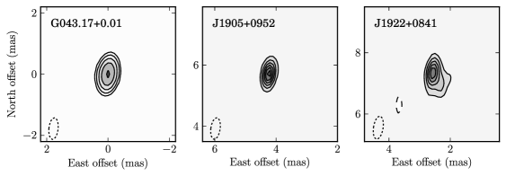
Figure 1: Images of the H₂O maser reference spot at $V_{\rm LSR}$ of –4.75 km s^-1 and the extragalactic radio sources used for the parallax measurements of W49N (G043.16$+$0.01) at the last epoch (2011 April 18). Source names are in the upper left corner and the restoring beam (dotted ellipse) is in the lower left corner of each panel. Contour levels for G043.16$+$0.01 maser emission are 250 Jy beam^-1 $\times 2^{n}$, $n$ = 0 …5, and for the background sources (J1905$+$0952 and J1922$+$0841) are spaced linearly at 0.02 and 0.20 mJy beam^-1, respectively.

W49N (G043.16$+$0.01) is a complex region of recent star formation containing the most luminous H₂O maser site in the Galaxy (Cheung et al., 1969; Burke et al., 1970). For the parallax measurement of W49N we phase-referenced to the maser spot at $V_{\rm LSR}$ of –4.75 km s^-1. Both background sources were detected at all epochs, except for J1922$+$0841 at the second epoch. Figure 1 shows images of the reference maser spot and the two background sources at the last epoch (BR145BC).

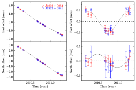
Figure 3: Parallax and proper motion data (markers) and best-fitting model (dotted line) for the maser spot at the $V_{\rm LSR}$ of –44.77 km s^-1 in W49N. Plotted are positions of the maser spots relative to the extragalactic radio sources J1905$+$0952 (circles), J1922$+$0841 (squares). Left panel: Eastward (upper panel) and northward (lower panel) offsets versus time. Right panel: Same as the left panel, except the best-fitting proper motion has been removed, displaying only the parallax signature.

We found 11 maser spots detected at all twelve epochs that could be used for precision astrometry. These maser spots cluster in six locations identified with letters A through F in Figure 2. Table 3 shows the independent and combined parallax fits for those maser spots. Figure 3 shows the independent parallax fit of the maser spot at $V_{\rm LSR}$ of –44.77 km s^-1 with each background source as an example. The combined parallax estimate is $0.090\pm 0.006$ mas, corresponding to a distance of $11.11^{+0.79}_{-0.69}$ kpc. The quoted parallax uncertainty is the formal fitting error multiplied by $\sqrt{11}$, assuming conservatively 100% correlated position uncertainties among the spots.

Our distance to W49N is consistent with that of $11.4\pm 1.2$ kpc obtain by Gwinn et al. (1992) by modeling the expansion (basically comparing maser Doppler velocities and proper motions). Combining the data for the two background sources, we measured the absolute proper motion of the reference maser spot to be $\mu_{x}$ = –4.49 $\pm$ 0.13 mas yr^-1 and $\mu_{y}$ = –6.42 $\pm$ 0.12 mas yr^-1, where $\mu_{x}=\mu_{\alpha}\cos\delta$ and $\mu_{y}=\mu_{\delta}$.

In order to model the internal motions of the masers to obtain the motion of the exciting star(s), we used 345 maser spots which appeared at four or more epochs within one year, and estimated their motions with respective to the reference maser spot. Figure 4 shows the motions with their mean value removed, which indicates an expansion originating from a small region that might include one (or more) young stellar object(s), as suggested by Gwinn et al. (1992). We fitted the data to models of expansion, with and without rotation. The estimated parameters from a Bayesian fitting procedure described by Sato et al. (2010) are listed in Table 4.

The motion of the expansion center relative to the reference maser spot from the two models are in good agreement within their joint uncertainties. We adopt the results from the simpler model A as the best estimate of the systematic motion. Converting the ($V_{0x}$, $V_{0y}$) to angular motions yields $\mu_{x}$ = 2.01 $\pm$ 0.08 and $\mu_{y}$ = 1.16 $\pm$ 0.06 mas yr^-1 at the parallax distance of 11.1 kpc to W49N. Adding this motion to the absolute motion of the reference maser spot, we estimate an absolute proper motion of the exciting star(s) of W49N to be $\mu_{x}$ = –2.48 $\pm$ 0.15 mas yr^-1 and $\mu_{y}$ = –5.27 $\pm$ 0.13 mas yr^-1. We note that the difference in proper motions of a maser spot provided by different background sources are larger than their formal errors for the individual fits. This difference could result from small structural variations such as jet motions in the background source or from unmodeled atmospheric delays.

4.2 G048.60$+$0.02

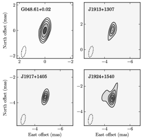
Figure 5: Images of the H₂O maser reference spot at $V_{\rm LSR}$ of +25.58 km s^-1 and the extragalactic radio sources used for the parallax measurements of G048.60$+$0.02 at the first epoch (2010 March 13). Source names are in the upper left corner and the restoring beam (dotted ellipse) is in the lower left corner of each panel. Contour levels for G048.60$+$0.02 maser emission are 5 Jy beam^-1 $\times~{}2^{n}$, $n$ = 0 …5, and for the background sources (J1913$+$1307, J1917$+$1405 and J1924$+$1540) are spaced linearly at 0.01, 0.01 and 0.05 Jy beam^-1, respectively.

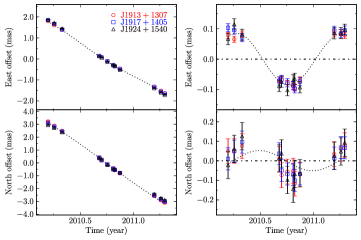
Figure 7: Parallax and proper motion data (markers) and a best-fitting model (dotted line) for the maser spot at the $V_{\rm LSR}$ of +24.31 km s^-1 in G048.60$+$0.02. Plotted are positions of the maser spot relative to the extragalactic radio sources J1913$+$1307 (circles), J1917$+$1405 (squares) and J1924$+$1540 (triangles). Left panel: Eastward (upper panel) and northward (lower panel) offsets versus time. Right panel: Same as the left panel, except the best-fitting proper motion has been removed, displaying only the parallax signature.

For the parallax measurement of G048.60$+$0.02, all the background sources were detected at all epochs after phase-referencing to the maser spot at $V_{\rm LSR}$ of +25.58 km s^-1. Figure 5 shows images of the reference maser spot and the background sources at epoch 1. Figure 6 shows the spatial distribution of H₂O maser spots and regions with maser spots used for the parallax fit. We found 9 maser spots that appeared at all epochs, which could be used for astrometric measurements. Table 5 shows the independent and combined solution for those maser spots. Figure 7 shows the parallax fit of maser spot at $V_{\rm LSR}$ of +24.31 km s^-1 with each background source as an example. The combined parallax estimate is $0.093\pm 0.005$ mas, corresponding to a distance of $10.75^{+0.61}_{-0.55}$ kpc. The quoted parallax uncertainty is the formal fitting error multiplied by $\sqrt{9}$, allowing for the possibility that position uncertainties of maser spots are entirely correlated. The absolute proper motion of the reference maser spot is estimated to be $\mu_{x}$ = –3.19 $\pm$ 0.01 mas yr^-1 and $\mu_{y}$ = –5.61 $\pm$ 0.03 mas yr^-1.

We found 55 maser spots that were detected in at least four epochs over one year and estimated their relative motions with respect to the reference maser spot. Figure 8 shows these motions with their mean value removed. Similar to the kinematic modeling of W49N, we fitted the data to expansion models with and without rotation. The estimated parameters are listed in Table 6. Owing to the large uncertainty of the parameters for rotation, we adopted the results from model A. The proper motion of the expansion center relative to the reference maser spot corresponds to $\mu_{x}$ = 0.30 $\pm$ 0.08 mas yr^-1 and $\mu_{y}$ = 0.11 $\pm$ 0.08 mas yr^-1 at a distance of 10.7 kpc. Adding this to the absolute motion of the reference maser spot, we obtained an absolute proper motion of the exciting star of G048.60$+$0.02 to be $\mu_{x}$ = –2.89 $\pm$ 0.08 mas yr^-1 and $\mu_{y}$ = –5.50 $\pm$ 0.09 mas yr^-1.

5 DISCUSSION

5.1 Inner portion of the Perseus arm traced by H₂O maser sources

Spiral arms in the Galaxy can be identified as large-scale features in longitude-velocity ($\ell-v$) diagrams from CO surveys (e.g., Dame et al. 1986). We therefore assign our masers to arms by associated them with molecular clouds, without possible bias by using distance and a model of spiral structure. A secure arm assignment requires that the position and velocity of the maser and the molecular cloud be in agreement with the position-velocity ($\ell-v$) locus of the arm. Using the data from the ¹³CO Galactic Ring Survey (GRS) by Jackson et al. (2006) and the APEX Telescope Large Area Survey of the GALaxy (ATLASGAL, Schuller et al. 2009), we determined that both G043.16$+$0.01 and G048.60$+$0.02 are nearly coincident on the sky with giant molecular clouds (see Figure 9). The clouds have small angular sizes ($\approx$ 3′), relatively large composite linewidths (FWHM 9.4 and 5.0 km s^-1, respectively), and low positive LSR velocities (11.1 and 17.7 km s^-1, respectively) which are consistent with the $\ell-v$ locus identified by Vallée (2008) for the Perseus arm.

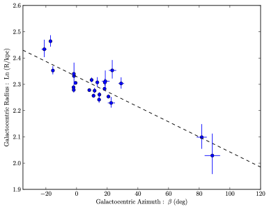
Figure 10: Pitch angle of Perseus arm. The logarithm of Galactocentric radius, $R$ (in kpc units) is plotted against Galactocentric longitude ($\beta$). The dashed line is a weighted fit to all the points and corresponds to a pitch angle of 9.5^∘.

Combining the two sources in the inner portion of the Perseus arm reported here with 22 sources with parallax measurements in the outer portion of the Perseus arm from the BeSSeL Survey, the Japanese VLBI Exploration of Radio Astrometry (VERA) project and the European VLBI Network (Y. K. Choi et al. 2013, in preparation), there are now 24 sources defining the locus of the Perseus arm. Figure 10 plots log($R$) versus $\beta$ for these sources, where $R$ and $\beta$ are Galactocentric radius and azimuth ($\beta$ is defined as 0^∘ toward the Sun and increasing with Galactic longitude). As shown in Figure 11, these sources are consistent with following a spiral from $\beta$ $\approx$ –25^∘ to 90^∘ (corresponding to Galactic longitude $\ell\approx$ 240^∘ to 43^∘) and extending nearly 15 kpc in length.

Using a Bayesian fitting approach that takes into account uncertainties in distance that maps into both R and $\beta$ (M. J. Reid 2013 et al. 2013, in preparation) and is insensitive to outliers (Sivia & Skilling, 2006, see “coservative formulation”), we estimate a global pitch angle of 9.5^∘ $\pm$ 1.3^∘ for the Perseus arm, which is in good agreement with that of 8.9^∘ $\pm$ 2.1^∘ determined from the 22 sources confined to the outer portion of the Perseus arm. As we can see from Figure 10, G043.16$+$0.01 and G048.60$+$0.02 at $\beta$ $\geq$ 80^∘ are crucial constraints for fitting a global pitch angle, since most of the sources are located at $\beta$ $\leq$ 25^∘. The preliminary pitch angle based on four sources in the Perseus arm in Reid et al. (2009b) of 16.5^∘ $\pm$ 3.1^∘ employed a simpler least-squares fitting approach in which only the residual in Galactocentric radius was minimized (when fitting a straight line to log($R$) versus $\beta$). Refitting the data from the four sources available in Reid et al. (2009b) with the new Bayesian approach, which accounts for error in both log($R$) and $\beta$, yields 15.1^∘ $\pm$ 6.1^∘. Thus the preliminary fit and our new fit, based on 24 sources, agree within their joint uncertainty.

5.2 3D motion in the inner portion of the Perseus arm

Combining the parallax and proper motion measurements with the systemic $V_{\rm LSR}$ (as listed in Table 7) enable us to determine the three-dimensional (3D) peculiar motions (relative to circular motion around the Galactic center) of G043.16$+$0.01 and G048.60$+$0.02. The $V_{\rm LSR}$ of G043.16$+$0.01 estimated from maser kinematics modeling (see Table 4) is about 11 km s^-1, which is consistent with that of 11 km s^-1 estimated for the molecular cloud. Similarly for G048.60$+$0.02 we estimate a $V_{\rm LSR}$ of 20 km s^-1 from kinematic modeling of masers (see Table 6), which is also close to the cloud velocity of 18 km s^-1. To allow for a difference of $V_{\rm LSR}$ between H₂O and CO, we assign a $V_{\rm LSR}$ uncertainty of 5 km s^-1. Similarly, there might be additional uncertainty referring those maser motions to that of the central star as reported in § 4. To account for this, we added a proper motion error floor corresponding to 5 km s^-1 to the measurement uncertainty in quadrature. The final adopted astrometric parameters and their uncertainties are listed in Table 7.

Assuming a flat rotation curve for the Milky Way with a rotation speed of LSR $\Theta_{0}$ = $239$ km s^-1, the distance to the Galactic center of $R_{0}$ = $8.3$ kpc (Brunthaler et al., 2011), and the solar motion of ($U_{\odot}$=$11.1$, $V_{\odot}$=$12.24$, $W_{\odot}$=$7.25$) km s^-1 from revised Hipparcos measurements by Schönrich et al. (2010), we estimated peculiar motions for the sources using the procedure described in Reid et al. (2009b). In order to obtain realistic uncertainties for peculiar motions, we include the effects of uncertainties in parallax, proper motion and $V_{\rm LSR}$. We do this by generating 10,000 random trials consistent with our measured values and (Gaussianly distributed) uncertainties. The ($U_{s}$,$V_{s}$,$W_{s}$) components of peculiar motion toward the Galactic center, in the direction of Galactic rotation, and toward the north Galactic pole, respectively, are given in Table 7. All components are consistent with zero motion, albeit with fairly large uncertainties owing to the great distances of the sources.

5.3 Distance to G048.60$+$0.02

Nagayama et al. (2011) also measured an H₂O maser parallax distance for G048.60$+$0.02 of $5.03\pm 0.19$ kpc using the VERA array. This result is significantly different from our distance of 10.75${}^{+0.61}_{-0.55}$ kpc. The Nagayama distance would place G048.60$+$0.02 in the Sagittarius-Carina arm and near (projected separation $\approx$ 1^∘) the supernova remnant G049.49-0.37 and the active star-forming region W51, which has several parallax distance measurements near 5.3 kpc (Xu et al., 2009; Sato et al., 2010; Wu et al., 2013). Note that the $V_{\rm LSR}$ of 18 km s^-1 for G048.60$+$0.02 is offset by $\approx 50$ km s^-1 from the W51 sources. This is inconsistent with the spiral arm assignment of G048.60$+$0.02 to the inner portion of the Perseus arm (described in § 5.1 and based on ¹³CO position–velocity information). Nagayama et al. (2011) suggested that the large velocity offset might be the result of the multiple SN explosions in W51. However, this is inconsistent with N-body simulations by Baba et al. (2009), which suggest that the acceleration by the SN explosion does not cause motions of that magnitude for swept-up, star-forming gas.

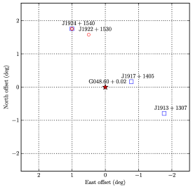
Figure 12: Sky positions of the target and background sources for G048.60$+$0.02. Squares/Circles denote background sources used in the VLBA/VERA observations.

Generally there is excellent agreement between parallaxes measured by different VLBI arrays. What could explain this unusual difference? Our VLBA parallax measurement has some superiorities over those of Nagayama et al. (2011). Firstly, our observations have longer interferometric baselines. Secondly, our observations have more and closer background sources, nearly symmetrically distributed relative to the target as shown in Figure 12. This could be very important to reduce systematic error due to unmodeled tropospheric delays. Note that the background sources used by Nagayama are very close together and both are offset mostly north of G048.60$+$0.02. Therefore, unmodeled tropospheric delays will be similar for both of their background sources. Noting this source of correlation, as well as the nearly 100% correlation among different maser spot positions, owing to nearly identical unmodeled tropospheric delays, the (formal) parallax uncertainty quoted by Nagayama of $\pm 0.007$ mas, may be underestimated by factors of $\sqrt{9}$ and $\sqrt{2}$ (for 9 maser spots and 2 background sources) and more realistically is $\pm 0.030$ mas. However, even with this uncertainty, the difference between our and Nagayama’s parallaxes ($0.103\pm 0.031$) is still somewhat significant. Thirdly, our observing epochs symmetrically sample the peaks of the sinusoidal parallax signature in right ascension, yielding near-zero correlation coefficients between parallax and proper motion terms. For these reasons, we suspect that our measured distance of 10.75${}^{+0.61}_{-0.55}$ kpc to G048.60$+$0.02 is more reliable.

5.4 A Star Formation Gap in the Perseus arm

As shown in Figure 10, we have yet to locate a high-mass star forming region with $\beta$ between $\approx$ 30^∘ and 80^∘ in the Perseus arm. Although we observed sources whose sky positions and velocities suggested kinematic distances in the Perseus arm, all were found to be much closer and located in the Local arm (Xu et al., 2013). In Figure 13, we plot the Galactic plane locations (based on kinematic distances) of $\approx$ 200 22-GHz H₂O masers stronger than 10 Jy and associated with star-forming regions. We find that the section of the Perseus arm between $\ell\approx$ 50^∘ to 80^∘ near the Solar Circle has very few 22 GHz candidate H₂O masers, even though they are numerous masers outside the Solar Circle in the Perseus arm for $\ell\geq$ 90^∘.

As shown in Figure 14, CO emission indicates that the Perseus arm can be seen from $\ell\approx$ 180^∘to 48^∘, where it spirals to the Solar Circle and $V_{\rm LSR}$ values approach zero and merge with local emission. The longitude range 64^∘ to 76^∘ is weak in CO emission (as it is from 160^∘ to 168^∘). This suggests that the Perseus arm, at least between $\ell\approx$ 64^∘ and 76^∘, is low in giant molecular clouds and massive star formation. Also plotted is the Galactic distribution of Massive Young Stellar Objects (MYSOs) from the Red MSX Sources (RMS) Survey (Urquhart et al., 2007). Since MYSOs are indicators of star formation, the small numbers of MYSOs at 50^∘ $<\ell<$ 80^∘ also indicates low levels of star formation in this portion of the Perseus arm.

6 SUMMARY

We measured trigonometric parallaxes and proper motions of H₂O masers in two star-forming regions, G043.16$+$0.01 and G048.60$+$0.02. We establish that both sources are at great distances and that G043.16$+$0.01 is one of the most luminous star forming regions in the Milky Way. These two sources have positions and $V_{\rm LSR}$’s that match ¹³CO emission from giant molecular clouds that are located in the Perseus arm. Thus, our parallax distances accurately locate the inner portion of the Perseus arm within the Milky Way. Combining our results with other parallax measurements for maser sources associated with the outer portion of the Perseus arm, we determined a global pitch angle of 9.3^∘ $\pm$ 1.3^∘ for the Perseus arm. Finally, we suggest that there is little massive-star formation in the Perseus arm between $l\approx 50$^∘ and 80^∘.

Table 1: VLBA Observations

Epoch	Program	Date	Antennas Available
group	code	(yyyy mm dd)	BR FD HN KP LA MK NL OV PT SC
1	BR145B1	2010 03 13	$\sqrt{}$   $\sqrt{}$   $\sqrt{}$   $\sqrt{}$   $\sqrt{}$   $\sqrt{}$   $\sqrt{}$   $\sqrt{}$   $\sqrt{}$   $\sqrt{}$
1	BR145B2	2010 04 03	$\sqrt{}$   $\sqrt{}$   $\sqrt{}$   $\sqrt{}$   $\sqrt{}$   $\sqrt{}$   $\sqrt{}$   $\sqrt{}$   $\sqrt{}$   $\sqrt{}$
1	BR145B3	2010 04 30	$\sqrt{}$   $\sqrt{}$   $\sqrt{}$   $\sqrt{}$   $\sqrt{}$   $\sqrt{}$   $\sqrt{}$   $\sqrt{}$   $\sqrt{}$   $\sqrt{}$
2	BR145B4	2010 09 05	$\sqrt{}$   $\sqrt{}$   $\sqrt{}$   $\sqrt{}$   $\sqrt{}$   $\sqrt{}$   $\sqrt{}$   $\sqrt{}$   $\sqrt{}$   $\sqrt{}$
2	BR145B5	2010 09 12	$\sqrt{}$   $\sqrt{}$   $\sqrt{}$   $\sqrt{}$   $\sqrt{}$   $\sqrt{}$   $\sqrt{}$   $\sqrt{}$   $\sqrt{}$   $\sqrt{}$
2	BR145B6	2010 10 03	$\sqrt{}$   $\sqrt{}$   $\sqrt{}$   $\sqrt{}$   $\sqrt{}$   $\sqrt{}$   $\sqrt{}$   $\sqrt{}$   $\sqrt{}$   $\sqrt{}$
2	BR145B7	2010 10 23	$\sqrt{}$   $\sqrt{}$   $\sqrt{}$   $\sqrt{}$   $\sqrt{}$   $\sqrt{}$   $\sqrt{}$   $\sqrt{}$   $\sqrt{}$   $\sqrt{}$
2	BR145B8	2010 10 28	$\sqrt{}$   $\sqrt{}$   $\sqrt{}$   $\sqrt{}$   $\sqrt{}$   $\sqrt{}$   $\sqrt{}$   $\sqrt{}$   $\sqrt{}$   $\sqrt{}$
2	BR145B9	2010 11 15	$\sqrt{}$   $\sqrt{}$   $\sqrt{}$   $\sqrt{}$   $\sqrt{}$   $\sqrt{}$   $\sqrt{}$   $\sqrt{}$   $\sqrt{}$   $\sqrt{}$
3	BR145BA	2011 03 13	$\sqrt{}$   $\sqrt{}$   $\sqrt{}$   $\sqrt{}$   $\sqrt{}$   $\sqrt{}$   $\sqrt{}$   $\sqrt{}$   $\sqrt{}$   $\sqrt{}$
3	BR145BB	2011 04 05	$\sqrt{}$   $\sqrt{}$   $\sqrt{}$   $\sqrt{}$   $\sqrt{}$   $\sqrt{}$   $\sqrt{}$   $\sqrt{}$   $\sqrt{}$   $\sqrt{}$
3	BR145BC	2011 04 18	$\sqrt{}$   $\sqrt{}$   $\sqrt{}$   $\sqrt{}$   $\sqrt{}$   $\sqrt{}$   $\sqrt{}$   $\sqrt{}$   $\sqrt{}$   $\sqrt{}$

Note. — The first column lists the epoch group number, which denotes the order number of peaks in the two year sinusoidal trigonometric parallax signature. Check marks indicate that the antenna produced good data, while a blank indicates that little or no useful data was obtained. Antenna codes are BR: Brewster, WA; FD: Fort Davis, TX; HN: Hancock, NH; KP: Kitt Peak, AZ; LA: Los Alamos, NM; MK: Mauna Kea, HI; NL: North Liberty, IA; OV: Owens Valley, CA; PT: Pie Town, NM; and SC: Saint Croix, VI.

Table 2: Source characteristics

Source	R.A. (J2000)	Dec. (J2000)	$\theta_{sep}$	P.A.	$S$	$V_{\rm LSR}$	Beam
	(h   m   s)	(°   ′   ″)	(°)	(°)	(Jy beam-1)	(km s-1)	(mas  mas  °)
G043.16$+$0.01	19 10 13.4096	+09 06 12.803	…	…	1000$-$8000	–4.75	0.8 $\times$ 0.4 @ 0–0
J1905+0952	19 05 39.8989	+09 52 08.407	1.4	–56	0.050$-$0.170		0.7 $\times$ 0.3 @ 0–8
J1922+0841	19 22 18.6337	+08 41 57.373	3.0	+98	0.010$-$0.020		0.9 $\times$ 0.3 @ 0–9
G048.60$+$0.02	19 20 31.1761	+13 55 25.209	…	…	90$-$160	+25.58	0.8 $\times$ 0.3 @ 0–9
J1917+1405	19 17 18.0641	+14 05 09.769	0.8	–78	0.020$-$0.050		0.8 $\times$ 0.3 @ –13
J1913+1307	19 13 18.0641	+13 07 47.331	1.9	–114	0.010$-$0.050		0.8 $\times$ 0.3 @ –12
J1924+1540	19 24 39.4559	+15 40 43.941	2.0	+30	0.090$-$0.450		0.8 $\times$ 0.3 @ –12

Note. — Column 1 gives the names of the maser sources and its corresponding background sources. Columns 2 to 3 list the absolute positions of the reference maser spot and background sources. Columns 4 to 5 give the separations ($\theta_{sep})$ and position angles (P.A.) east of north between maser and background sources. Columns 6 to 7 give the brightnesses ($S$) and $V_{\rm LSR}$ of reference maser spot. The last column gives the full width at half maximum (FWHM) size and P.A. of the Gaussian restoring beam. Calibrators are from the BeSSeL calibrator survey (Immer et al., 2011).

Table 3: Parallax and proper motion fits for W49N 

Background	Region	$V_{\rm LSR}$	Parallax	$\mu_{x}$	$\mu_{y}$	$\Delta x$	$\Delta y$	$\chi^{2}_{\nu}$	$\sigma_{x}$	$\sigma_{y}$
source		(km s-1)	(mas)	(mas yr-1)	(mas yr-1)	(mas)	(mas)		(mas)	(mas)
J1905$+$0952	B	012.95	0.096 $\pm$ 0.008	–2.86 $\pm$ 0.02	–5.44 $\pm$ 0.01	–57.87 $\pm$ 0.01	270.85 $\pm$ 0.01	1.001	0.025	0.017
	A	012.95	0.102 $\pm$ 0.006	–2.90 $\pm$ 0.01	–5.72 $\pm$ 0.02	–41.09 $\pm$ 0.01	62.44 $\pm$ 0.01	0.984	0.018	0.024
	C	008.31	0.095 $\pm$ 0.007	–2.80 $\pm$ 0.02	–5.94 $\pm$ 0.04	–21.86 $\pm$ 0.01	–9.88 $\pm$ 0.01	0.994	0.022	0.049
	C	007.89	0.082 $\pm$ 0.006	–2.93 $\pm$ 0.02	–5.94 $\pm$ 0.06	–21.89 $\pm$ 0.01	–9.73 $\pm$ 0.02	0.993	0.019	0.078
	E	004.94	0.080 $\pm$ 0.007	–2.51 $\pm$ 0.02	–5.16 $\pm$ 0.01	31.43 $\pm$ 0.01	308.78 $\pm$ 0.00	0.953	0.024	0.012
	E	004.52	0.084 $\pm$ 0.007	–2.50 $\pm$ 0.02	–5.17 $\pm$ 0.01	31.44 $\pm$ 0.01	308.77 $\pm$ 0.00	0.969	0.024	0.011
	E	001.99	0.084 $\pm$ 0.004	–2.53 $\pm$ 0.01	–5.33 $\pm$ 0.01	29.22 $\pm$ 0.00	299.72 $\pm$ 0.01	0.996	0.012	0.013
	C	–11.07	0.100 $\pm$ 0.012	–3.08 $\pm$ 0.03	–5.55 $\pm$ 0.02	–2.08 $\pm$ 0.01	–4.18 $\pm$ 0.01	0.991	0.039	0.022
	F	–44.77	0.087 $\pm$ 0.007	–2.94 $\pm$ 0.02	–5.05 $\pm$ 0.02	–61.71 $\pm$ 0.01	196.77 $\pm$ 0.01	0.991	0.022	0.020
	D	–46.04	0.083 $\pm$ 0.005	–3.07 $\pm$ 0.01	–5.98 $\pm$ 0.03	–9.00 $\pm$ 0.00	–299.53 $\pm$ 0.01	0.978	0.016	0.033
	D	–46.46	0.081 $\pm$ 0.006	–3.06 $\pm$ 0.01	–6.03 $\pm$ 0.02	–8.98 $\pm$ 0.01	–299.52 $\pm$ 0.01	0.975	0.018	0.020
J1922$+$0841	B	012.95	0.102 $\pm$ 0.007	–2.95 $\pm$ 0.02	–5.25 $\pm$ 0.04	–56.06 $\pm$ 0.01	269.15 $\pm$ 0.02	0.969	0.016	0.046
	A	012.95	0.111 $\pm$ 0.007	–2.99 $\pm$ 0.02	–5.55 $\pm$ 0.03	–39.29 $\pm$ 0.01	60.75 $\pm$ 0.01	0.976	0.017	0.034
	C	008.31	0.102 $\pm$ 0.005	–2.88 $\pm$ 0.01	–5.77 $\pm$ 0.06	–20.06 $\pm$ 0.00	–11.57 $\pm$ 0.02	0.999	0.011	0.064
	C	007.89	0.089 $\pm$ 0.006	–3.01 $\pm$ 0.02	–5.77 $\pm$ 0.07	–20.08 $\pm$ 0.01	–11.43 $\pm$ 0.02	0.981	0.015	0.074
	E	004.94	0.092 $\pm$ 0.006	–2.60 $\pm$ 0.01	–4.98 $\pm$ 0.04	33.24 $\pm$ 0.01	307.09 $\pm$ 0.01	0.969	0.013	0.041
	E	004.52	0.098 $\pm$ 0.006	–2.59 $\pm$ 0.01	–4.99 $\pm$ 0.04	33.25 $\pm$ 0.01	307.07 $\pm$ 0.01	0.973	0.014	0.039
	E	001.99	0.092 $\pm$ 0.008	–2.62 $\pm$ 0.02	–5.14 $\pm$ 0.05	31.03 $\pm$ 0.01	298.03 $\pm$ 0.02	0.981	0.021	0.049
	C	–11.07	0.103 $\pm$ 0.009	–3.17 $\pm$ 0.02	–5.36 $\pm$ 0.05	–0.27 $\pm$ 0.01	–5.87 $\pm$ 0.02	0.992	0.025	0.053
	F	–44.77	0.099 $\pm$ 0.006	–3.03 $\pm$ 0.01	–4.88 $\pm$ 0.03	–59.91 $\pm$ 0.01	195.08 $\pm$ 0.01	0.974	0.013	0.035
	D	–46.04	0.090 $\pm$ 0.007	–3.16 $\pm$ 0.02	–5.81 $\pm$ 0.04	–7.19 $\pm$ 0.01	–301.23 $\pm$ 0.01	0.973	0.018	0.038
	D	–46.46	0.089 $\pm$ 0.008	–3.15 $\pm$ 0.02	–5.85 $\pm$ 0.04	–7.18 $\pm$ 0.01	–301.21 $\pm$ 0.01	0.993	0.021	0.039
Combined
	all		0.090 $\pm$ 0.006					0.970	0.026	0.051

Note. — Absolute proper motions are defined as ${\mu_{x}}=\mu_{\alpha\cos{\delta}}$ and ${\mu_{y}}=\mu_{\delta}$. $\chi^{2}_{\nu}$ is reduced $\chi^{2}$ of post-fit residuals, $\sigma_{x}$ and $\sigma_{y}$ are error floor in $x$ and $y$, respectively.

Table 4: Best-fitting models for H₂O maser kinematics in W49N

Parameter				Model
	Type	Unit		A	B
Velocity	$V_{0x}$	km s-1		101.34 $\pm$ 4.02	106.27 $\pm$ 4.28
	$V_{0y}$	km s-1		61.30 $\pm$ 2.58	57.92 $\pm$ 3.13
	$V_{0z}$	km s-1		10.73 $\pm$ 1.40	10.55 $\pm$ 1.28
Position	$x_{0}$	arcsec		0.37 $\pm$ 0.08	0.23 $\pm$ 0.08
	$y_{0}$	arcsec		0.06 $\pm$ 0.08	–0.11 $\pm$ 0.13
Expansion	$V_{\rm exp}$	km s-1		16.77 $\pm$ 1.80	10.99 $\pm$ 1.33
	$\gamma$			0.60 $\pm$ 0.06	0.81 $\pm$ 0.06
Rotation	$V_{\rm rot}$	km s-1		0	5.28 $\pm$ 0.80
	$\theta$	radian		0	0.48 $\pm$ 0.72
	$\phi$	radian		0	1.68 $\pm$ 0.30

Note. — Model A includes only radial motions. Model B includes radial and rotation motions.

Table 5: Parallax and proper motion fits for G048.60$+$0.02 

Background	Region	$V_{\rm LSR}$	Parallax	$\mu_{x}$	$\mu_{y}$	$\Delta x$	$\Delta y$	$\chi^{2}_{\nu}$	$\sigma_{x}$	$\sigma_{y}$
source		(km s-1)	(mas)	(mas yr-1)	(mas yr-1)	(mas)	(mas)		(mas)	(mas)
J1913$+$1307	A	25.58	0.098 $\pm$ 0.003	–3.11 $\pm$ 0.01	–5.80 $\pm$ 0.02	2.81 $\pm$ 0.00	–4.68 $\pm$ 0.01	0.994	0.010	0.027
	A	25.16	0.097 $\pm$ 0.003	–3.12 $\pm$ 0.01	–5.77 $\pm$ 0.02	2.81 $\pm$ 0.00	–4.71 $\pm$ 0.01	0.996	0.009	0.026
	A	24.74	0.082 $\pm$ 0.003	–3.12 $\pm$ 0.01	–5.76 $\pm$ 0.07	2.82 $\pm$ 0.00	–4.79 $\pm$ 0.02	0.999	0.010	0.084
	A	24.31	0.086 $\pm$ 0.003	–3.12 $\pm$ 0.01	–5.77 $\pm$ 0.05	2.82 $\pm$ 0.00	–4.77 $\pm$ 0.02	0.997	0.009	0.063
	B	20.52	0.088 $\pm$ 0.004	–2.67 $\pm$ 0.01	–5.68 $\pm$ 0.02	131.04 $\pm$ 0.00	–69.53 $\pm$ 0.01	0.996	0.011	0.029
	B	20.10	0.085 $\pm$ 0.003	–2.67 $\pm$ 0.01	–5.68 $\pm$ 0.02	131.03 $\pm$ 0.00	–69.54 $\pm$ 0.01	0.988	0.010	0.028
	B	19.68	0.077 $\pm$ 0.003	–2.69 $\pm$ 0.01	–5.66 $\pm$ 0.02	131.01 $\pm$ 0.00	–69.58 $\pm$ 0.01	0.938	0.009	0.028
	B	19.26	0.089 $\pm$ 0.004	–2.72 $\pm$ 0.01	–5.72 $\pm$ 0.02	130.04 $\pm$ 0.00	–72.30 $\pm$ 0.01	1.009	0.013	0.026
	B	18.84	0.089 $\pm$ 0.004	–2.73 $\pm$ 0.01	–5.72 $\pm$ 0.02	130.05 $\pm$ 0.00	–72.30 $\pm$ 0.01	1.002	0.013	0.027
J1917$+$1405	A	25.58	0.105 $\pm$ 0.004	–3.18 $\pm$ 0.01	–5.64 $\pm$ 0.02	2.98 $\pm$ 0.00	0.48 $\pm$ 0.01	0.994	0.013	0.028
	A	25.16	0.104 $\pm$ 0.004	–3.19 $\pm$ 0.01	–5.61 $\pm$ 0.02	2.98 $\pm$ 0.00	0.45 $\pm$ 0.01	0.998	0.012	0.028
	A	24.74	0.089 $\pm$ 0.004	–3.19 $\pm$ 0.01	–5.60 $\pm$ 0.06	3.00 $\pm$ 0.00	0.37 $\pm$ 0.02	0.999	0.012	0.077
	A	24.31	0.092 $\pm$ 0.004	–3.18 $\pm$ 0.01	–5.61 $\pm$ 0.05	2.99 $\pm$ 0.00	0.39 $\pm$ 0.02	0.997	0.012	0.057
	B	20.52	0.096 $\pm$ 0.004	–2.74 $\pm$ 0.01	–5.52 $\pm$ 0.01	131.21 $\pm$ 0.00	–64.37 $\pm$ 0.01	0.993	0.013	0.017
	B	20.10	0.093 $\pm$ 0.004	–2.74 $\pm$ 0.01	–5.52 $\pm$ 0.01	131.21 $\pm$ 0.00	–64.38 $\pm$ 0.00	0.979	0.013	0.015
	B	19.68	0.085 $\pm$ 0.004	–2.76 $\pm$ 0.01	–5.50 $\pm$ 0.02	131.19 $\pm$ 0.00	–64.42 $\pm$ 0.01	0.910	0.012	0.018
	B	19.26	0.097 $\pm$ 0.004	–2.79 $\pm$ 0.01	–5.57 $\pm$ 0.01	130.21 $\pm$ 0.00	–67.14 $\pm$ 0.00	0.995	0.014	0.015
	B	18.84	0.096 $\pm$ 0.004	–2.80 $\pm$ 0.01	–5.56 $\pm$ 0.01	130.22 $\pm$ 0.00	–67.14 $\pm$ 0.00	0.998	0.013	0.015
J1924$+$1540	A	25.58	0.106 $\pm$ 0.005	–3.28 $\pm$ 0.01	–5.44 $\pm$ 0.04	2.68 $\pm$ 0.00	0.00 $\pm$ 0.01	0.996	0.015	0.043
	A	25.16	0.104 $\pm$ 0.005	–3.28 $\pm$ 0.01	–5.41 $\pm$ 0.04	2.68 $\pm$ 0.00	–0.03 $\pm$ 0.01	0.998	0.015	0.048
	A	24.74	0.089 $\pm$ 0.005	–3.28 $\pm$ 0.01	–5.40 $\pm$ 0.07	2.69 $\pm$ 0.00	–0.11 $\pm$ 0.03	0.998	0.015	0.089
	A	24.31	0.093 $\pm$ 0.005	–3.28 $\pm$ 0.01	–5.41 $\pm$ 0.06	2.69 $\pm$ 0.00	–0.09 $\pm$ 0.02	0.998	0.016	0.070
	B	20.52	0.096 $\pm$ 0.005	–2.83 $\pm$ 0.01	–5.32 $\pm$ 0.03	130.91 $\pm$ 0.00	–64.84 $\pm$ 0.01	0.997	0.016	0.037
	B	20.10	0.093 $\pm$ 0.005	–2.83 $\pm$ 0.01	–5.32 $\pm$ 0.03	130.91 $\pm$ 0.00	–64.86 $\pm$ 0.01	0.994	0.016	0.037
	B	19.68	0.087 $\pm$ 0.006	–2.85 $\pm$ 0.02	–5.30 $\pm$ 0.03	130.89 $\pm$ 0.01	–64.90 $\pm$ 0.01	0.959	0.017	0.038
	B	19.26	0.097 $\pm$ 0.005	–2.89 $\pm$ 0.01	–5.36 $\pm$ 0.03	129.91 $\pm$ 0.00	–67.62 $\pm$ 0.01	0.997	0.015	0.037
	B	18.84	0.097 $\pm$ 0.005	–2.89 $\pm$ 0.01	–5.36 $\pm$ 0.03	129.92 $\pm$ 0.00	–67.62 $\pm$ 0.01	0.999	0.015	0.036
Combined
	all		0.093 $\pm$ 0.005					0.990	0.029	0.069

Note. — Absolute proper motions are defined as ${\mu_{x}}=\mu_{\alpha\cos{\delta}}$ and ${\mu_{y}}=\mu_{\delta}$. $\chi^{2}_{\nu}$ is reduced $\chi^{2}$ of post-fit residuals, $\sigma_{x}$ and $\sigma_{y}$ are error floor in $x$ and $y$, respectively.

Table 6: Best-fitting models for H₂O maser kinematics in G048.60$+$0.02

Parameter				Model
	Type	Unit		A	B
Velocity	$V_{0x}$	km s-1		15.51 $\pm$ 3.96	25.00 $\pm$ 4.44
	$V_{0y}$	km s-1		5.44 $\pm$ 3.83	6.62 $\pm$ 3.65
	$V_{0z}$	km s-1		20.65 $\pm$ 2.64	19.24 $\pm$ 2.73
Position	$x_{0}$	arcsec		0.11 $\pm$ 0.09	–0.06 $\pm$ 0.11
	$y_{0}$	arcsec		–0.05 $\pm$ 0.09	0.01 $\pm$ 0.09
Expansion	$V_{\rm exp}$	km s-1		7.78 $\pm$ 2.91	9.25 $\pm$ 3.30
	$\gamma$			–0.26 $\pm$ 0.35	–0.23 $\pm$ 0.41
Rotation	$V_{\rm rot}$	km s-1		0	7.44 $\pm$ 8.45
	$\theta$	radian		0	1.48 $\pm$ 1.76
	$\phi$	radian		0	–1.46 $\pm$ 1.59

Note. — Model A includes only radial motions. Model B includes radial and rotation motions.

Table 7: Parallaxes and proper motions of H₂O maser sources located in Inner Perseus Arm

Source	Parallax	Distance	$\mu_{x}$	$\mu_{y}$	$V_{\rm LSR}$	$U_{s}$	$V_{s}$	$W_{s}$
name	(mas)	(kpc)	(mas yr-1)	(mas yr-1)	(km s-1)	(km s-1)	(km s-1)	(km s-1)
G043.16$+$0.01	0.090 $\pm$ 0.006	$11.11^{+0.79}_{-0.69}$	–2.48 $\pm$ 0.15	–5.27 $\pm$ 0.13	11 $\pm$ 5	–17 $\pm$ 11	–23 $\pm$ 16	–5 $\pm$ 8
G048.60$+$0.02	0.093 $\pm$ 0.005	$10.75^{+0.61}_{-0.55}$	–2.89 $\pm$ 0.13	–5.50 $\pm$ 0.13	18 $\pm$ 5	0–4 $\pm$ 11	013 $\pm$ 14	06 $\pm$ 7

Note. — Column 3 lists the parallax distance. Column 4 to 6 list absolute proper motion in eastward and northward direction and $V_{\rm LSR}$, respectively. Columns 7 to 9 list peculiar motion components, where $U_{s}$, $V_{s}$, $W_{s}$ are directed toward the Galactic center, in the direction of Galactic rotation and toward the North Galactic Pole (NGP), respectively. The peculiar motions were estimated using the Galactic parameters from Brunthaler et al. (2011) and solar motion parameters from Schönrich et al. (2010).

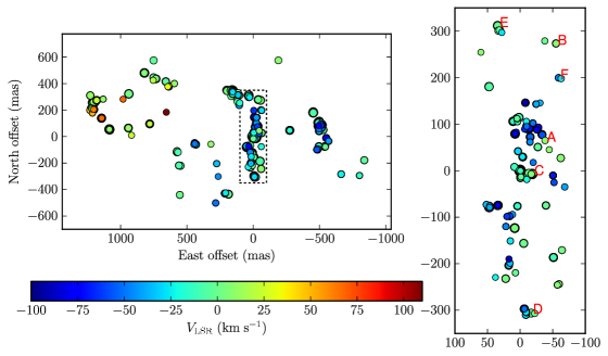
Figure 2: Left panel: spatial distribution of the H₂O maser spots (with brightness $\geq$ 50 Jy beam^-1 for a restoring beam of $\sim 3\times 1$ mas) toward W49N from VLBA observations at the last epoch (2011 April 18). Each maser spot is represented by a filled circle whose area is proportional to the logarithm of the flux density. Right panel: blow-ups of maser spots (with brightness $\geq$ 50 Jy beam^-1 for a restoring beam of $\sim 0.8\times 0.4$ mas) distribution in the field indicated with a dotted box in left panel. All the maser spots used for the parallax fit are from this field. Each region including maser feature used for parallax fit is labeled with a letter. The reference maser spot is located in region C. The color bar denotes the $V_{\rm LSR}$ range from –100 to +110 km s^-1.
(This figure is available in color in the electronic version.)

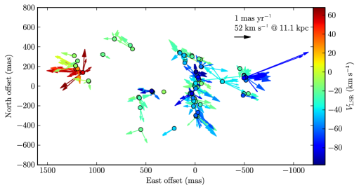
Figure 4: Averaged positions (circles) and relative motions (arrows) with mean value removed of maser spots respective to reference maser spot located at (0, 0) mas in W49N. The color bar denotes the $V_{\rm LSR}$ range from –98 to 68 km s^-1 of the maser features. The length and the direction of an arrow indicate the speed (given by the scale arrow in the upper right of the panel), the size of the arrow head is proportional to the uncertainty of the motion.
(This figure is available in color in the electronic version.)

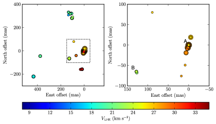
Figure 6: Left panel: spatial distribution of the H₂O maser spots (with brightness $\geq$ 1 Jy beam^-1 for a restoring beam of $\sim 3\times 1$ mas) toward G048.60$+$0.02 from VLBA observations at the first epoch (2010 March 13). Each maser spot is represented by a filled circle whose area is proportional to the logarithm of the flux density. Right panel: blow-ups of the maser spot distribution in the field indicated with a dotted box in the left panel. All the maser spots (with brightness $\geq$ 1 Jy beam^-1 for a restoring beam of $\sim 0.8\times 0.3$ mas) used for parallax fit are from this field. Each region including maser spot for parallax fit is labeled with a letter. The reference maser spot is in region A. The color bar denotes the $V_{\rm LSR}$ range from +8 to +36 km s^-1.
(This figure is available in color in the electronic version.)

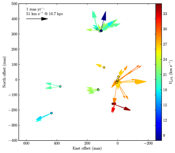
Figure 8: Averaged positions (circles) and relative motions (arrows) with mean value removed of maser spots relative to reference maser spot located at (0, 0) mas in G048.60$+$0.02. The color bar denotes the $V_{\rm LSR}$ range from 8 to 35 km s^-1 of the maser features. The length and the direction of an arrow indicate the speed (given by the scale arrow in the upper left of the panel), the size of the arrow head is proportional to the uncertainty of the motion.
(This figure is available in color in the electronic version.)

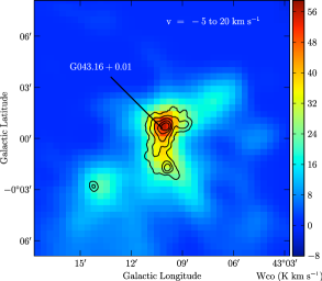
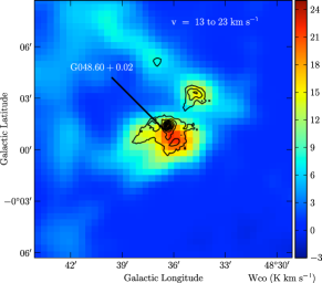
Figure 9: Velocity-integrated ¹³CO intensity for the molecular clouds apparently associated G043.16$+$0.01 (left panel) and G048.60$+$0.02 (right panel). The velocity integration ranges are indicated in the upper right of each figure. The data are from the Galactic Ring Survey (Jackson et al., 2006). Over plotted contours are for the 870 $\mu$m continuum emission from the APEX Telescope Large Area Survey of the Galaxy (ATLASGAL) (Schuller et al., 2009). Contour levels are start at 2 Jy beam^-1 and increase by factors of 2 for G043.16$+$0.01; they are linearly spaced at 1 Jy beam^-1 for G048.60$+$0.02.
(This figure is available in color in the electronic version.)

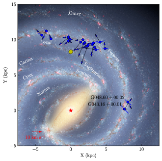
Figure 11: Location (dots with bar) and peculiar motion (arrows) projected on the Galactic plane of H₂O maser sources with parallax measurements in the Perseus arm. The length of the bar denotes the distance uncertainty. A 10 km s^-1 motion scale is in the lower left. The background is an artist’s conception of Milky Way (R. Hurt: NASA/JPL-Caltech/SSC) viewed from the north Galactic pole from which the Galaxy rotates clockwise. The Galactic center (red star) is at (0, 0) and the Sun (yellow dot) at (0, 8.3) kpc.
(This figure is available in color in the electronic version.)

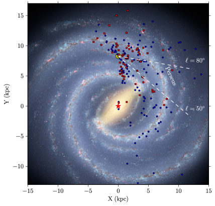
Figure 13: Galactic distributions of 22 GHz H₂O masers with kinematic distances (blue dots) from Valdettaro et al. (2001) and parallax distances (red squares) from M. J. Reid et al. (2013, in preparation). Kinematic distances have been used to generate these plots and distance ambiguities have been resolved using the prescription of Fish et al. (2003), based simply on Galactic latitude. Note that these kinematic distances are highly uncertain and are almost useless to determine spiral structure. The background is an artist’s conception of Milky Way (R. Hurt: NASA/JPL-Caltech/SSC) viewed from the north Galactic pole from which the Galaxy rotates clockwise. The Galactic center (red star) is at (0, 0) and the Sun (yellow dot) at (0, 8.3) kpc.
(This figure is available in color in the electronic version.)

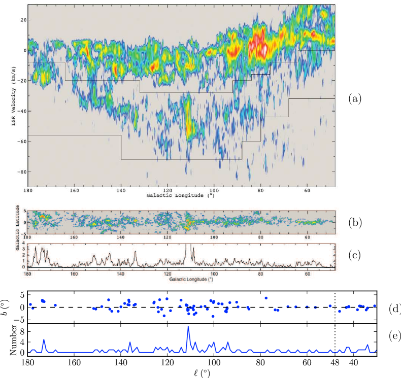
Figure 14: (a): A CO longitude-velocity diagram integrated over a 10^∘ strip of Galactic latitude centered on the Galactic plane from Dame et al. (2001). The solid lines roughly outline the locus of the Perseus arm. The colors indicate log intensity, from 0.1 K-arcdeg (blue) to 16 K-arcdeg (white). Below the right edge at longitude of 48^∘ the Perseus arm is inside the solar circle with small positive velocity and blends with stronger, more extensive local emission, and hence it is not shown. (b): A velocity-integrated CO map of the Perseus arm, obtained by integrating the Dame et al. (2001) survey over the velocity ranges indicated in (a). The colors indicate log Wco, from 1 K km s^-1 (blue) to 100 K km s^-1 (white). (c): Mean CO intensity of the Perseus arm vs. Galactic longitude, obtained by averaging the map in (b) over latitude. (d): Galactic longitude and latitude of Massive Young Stellar Objects (MYSOs) within the velocity ranges indicated in (a). These MYSOs are from the Red MSX Sources (RMS) Survey (%****␣ms.tex␣Line␣1400␣****http://www.ast.leeds.ac.uk/RMS/). (e): Distribution of Galactic longitude of MSYOs plotted in (d). The dotted line in (d) and (e) indicates longitude of 48^∘.
(This figure is available in color in the electronic version.)

References

- Baba et al. (2009) Baba, J., Asaki, Y., Makino, J., et al. 2009, ApJ, 706, 471
- Benjamin et al. (2005) Benjamin, R. A., Churchwell, E., Babler, B. L., et al. 2005, ApJ, 630, L149
- Brunthaler et al. (2011) Brunthaler, A., Reid, M. J., Menten, K. M., et al. 2011, Astronomische Nachrichten, 332, 461
- Burke et al. (1970) Burke, B. F., Papa, D. C., Papadopoulos, G. D., et al. 1970, ApJ, 160, L63
- Cheung et al. (1969) Cheung, A. C., Rank, D. M., Townes, C. H., Thornton, D. D., & Welch, W. J. 1969, Nature, 221, 626
- Churchwell et al. (2009) Churchwell, E., Babler, B. L., Meade, M. R., et al. 2009, PASP, 121, 213
- Dame et al. (1986) Dame, T. M., Elmegreen, B. G., Cohen, R. S., & Thaddeus, P. 1986, ApJ, 305, 892
- Dame et al. (2001) Dame, T. M., Hartmann, D., & Thaddeus, P. 2001, ApJ, 547, 792
- Deller et al. (2007) Deller, A. T., Tingay, S. J., Bailes, M., & West, C. 2007, PASP, 119, 318
- Drimmel (2000) Drimmel, R. 2000, A&A, 358, L13
- Fish et al. (2003) Fish, V. L., Reid, M. J., Wilner, D. J., & Churchwell, E. 2003, ApJ, 587, 701
- Gwinn et al. (1992) Gwinn, C. R., Moran, J. M., & Reid, M. J. 1992, ApJ, 393, 149
- Honma et al. (2012) Honma, M., Nagayama, T., Ando, K., et al. 2012, PASJ, 64, 136
- Immer et al. (2011) Immer, K., Brunthaler, A., Reid, M. J., et al. 2011, ApJS, 194, 25
- Jackson et al. (2006) Jackson, J. M., Rathborne, J. M., Shah, R. Y., et al. 2006, ApJS, 163, 145
- Kettenis et al. (2006) Kettenis, M., van Langevelde, H. J., Reynolds, C., & Cotton, B. 2006, in Astronomical Society of the Pacific Conference Series, Vol. 351, Astronomical Data Analysis Software and Systems XV, ed. C. Gabriel, C. Arviset, D. Ponz, & S. Enrique, 497
- Ma et al. (1998) Ma, C., Arias, E. F., Eubanks, T. M., et al. 1998, AJ, 116, 516
- Nagayama et al. (2011) Nagayama, T., Omodaka, T., Handa, T., et al. 2011, PASJ, 63, 719
- Reid et al. (2009a) Reid, M. J., Menten, K. M., Brunthaler, A., et al. 2009a, ApJ, 693, 397
- Reid et al. (2009b) Reid, M. J., Menten, K. M., Zheng, X. W., et al. 2009b, ApJ, 700, 137
- Sato et al. (2010) Sato, M., Reid, M. J., Brunthaler, A., & Menten, K. M. 2010, ApJ, 720, 1055
- Schönrich et al. (2010) Schönrich, R., Binney, J., & Dehnen, W. 2010, MNRAS, 403, 1829
- Schuller et al. (2009) Schuller, F., Menten, K. M., Contreras, Y., et al. 2009, A&A, 504, 415
- Sivia & Skilling (2006) Sivia, D. S., & Skilling, J. 2006, Data Analysis–A Bayesian Tutorial, 2nd edn. (Oxford Science Publications)
- Urquhart et al. (2007) Urquhart, J. S., Busfield, A. L., Hoare, M. G., et al. 2007, A&A, 461, 11
- Valdettaro et al. (2001) Valdettaro, R., Palla, F., Brand, J., et al. 2001, A&A, 368, 845
- Vallée (2008) Vallée, J. P. 2008, AJ, 135, 1301
- Wu et al. (2013) Wu, Y. W., Sato, M., Reid, M. J., et al. 2013, ApJ, submitted
- Xu et al. (2009) Xu, Y., Reid, M. J., Menten, K. M., et al. 2009, ApJ, 693, 413
- Xu et al. (2013) Xu, Y., Li, J. J., Reid, M. J., et al. 2013, ApJ, 769, 15
- Zhang et al. (2012) Zhang, B., Reid, M. J., Menten, K. M., & Zheng, X. W. 2012, ApJ, 744, 23