Quantum search on graphene lattices

Abstract

We present a continuous-time quantum search algorithm on a graphene lattice. This provides the sought-after implementation of an efficient continuous-time quantum search on a two-dimensional lattice. The search uses the linearity of the dispersion relation near the Dirac point and can find a marked site on a graphene lattice faster than the corresponding classical search. The algorithm can also be used for state transfer and communication.

Introduction.– Quantum walks Por13 ; Rei12 can provide polynomial and even exponential speed-up compared to classical random walks Aharonov et al. (1993); Kempe (2003); Kendon (2006); Santha (2008) and may serve as a universal computational primitive for quantum computation Childs (2009). This has led to substantial interest in the theoretical aspects of this phenomenon, as well as in finding experimental implementations Karski et al (2009); Schmitz et al (2009); Xue et al (2009); Zaehringer et al (2010); Perets et al (2009); Schreiber et al (2010). One of the most fascinating applications of quantum walks is their use in spatial quantum search algorithms first published for the search on the hypercube in Shenvi et al. (2003). Like Grover’s search algorithm Grover (1996, 1997) for searching an unstructured database, quantum walk search algorithms can achieve up to quadratic speed-up compared to the corresponding classical search. For quantum searches on $d$-dimensional square lattices, certain restrictions have been observed, however, depending on whether the underlying quantum walk is discrete Aharonov et al. (1993) or continuous FG98 . While effective search algorithms for discrete walks have been reported for $d\geq 2$ Ambainis et al. (2005); ADMP10 , continuous-time quantum search algorithms on square lattices show speed-up compared to the classical search only for $d\geq 4$ Childs and Goldstone (2004). This problem has been circumvented in Childs and Goldstone (2004), however, at the conceptual cost of adding internal degrees of freedom (spin) and a discrete Dirac equation.

Experimental implementations of discrete quantum walks need time stepping mechanisms such as laser pulses Karski et al (2009); Schmitz et al (2009); Xue et al (2009); Zaehringer et al (2010); Schreiber et al (2010). It is thus in general simpler to consider experimental realizations with continuous time evolution. However, in the absence of internal degrees of freedom, no known search algorithm on lattices exists up to now in the physically relevant regime $d=2$ or $3$. Finding such an algorithm is highly topical due to applications in secure state transfer and communication across regular lattices as demonstrated in Hein and Tanner (2009b).

We will show in the following that continuous-time quantum search in 2D is indeed possible! We will demonstrate that such a quantum search can be performed at the Dirac point in graphene. This is potentially of great interest, as graphene is now becoming available cheaply and can be fabricated routinely CN09 ; WA11 . Performing quantum search and quantum state transfer on graphene provides a new way of channeling energy and information across lattices and between distinct sites. Graphene sheets have been identified as a potential single-molecule sensor Sch07 ; Weh08 being very sensitive to a change of the density of states near the Dirac point. This property is closely related to the quantum search effect described in this paper.

Continuous-time quantum search algorithms take place on a lattice with a set of $N$ sites interacting via hopping potentials (usually between nearest neighbors only). Standard searches work at the ground state energy which, due to the periodicity of the lattice, is related to quasi-momentum $k=0$. After introducing a perturbation at one of the lattice sites, the parameters are adjusted such that an avoided crossing between the localized ‘defect’ state and the ground state is formed. The search is now performed in this two-level sub-system Hein and Tanner (2010a). Criticality with respect to the dimension is reached when the gap at the avoided crossing and the eigenenergy spacing near the crossing scale in the same way with $N$.

Continuous-time quantum walks (CTQW) FG98 operate in the position (site) space. If the states $\left|j\right\rangle$ represent the sites of the lattice, the Schrödinger equation governing the probability amplitudes $\alpha_{j}\left(t\right)=\left<j\right|\left.\psi(t)\right>$ is given by

$$\frac{d}{dt}\alpha_{j}\left(t\right)=-i\sum_{l=1}^{N}{H}_{jl}\alpha_{l}\left(t\right)$$ (1)

where the Hamiltonian ${\bf H}=\epsilon_{D}{\bf I}+v{\bf A}$ is of tight-binding type where $\bf A$ is the adjacency matrix of the lattice and $\bf I$ is the identity matrix, $\epsilon_{D}$ is the on-site energy and $v$ is the strength of the hopping potential. In Childs and Goldstone (2004), the walk Hamiltonian was set to be the discrete Laplacian where $v=-1$ and $\epsilon_{D}$ is the coordination number of the lattice. A marked site is then introduced by altering the on-site energy of that site. The system is initialized at $t=0$ in the ground state of the unperturbed lattice leading to an effective search for $d\geq 4$. For the search based on the discretized Dirac operator Childs and Goldstone (2004), an additional spin degree of freedom is introduced. This gives optimum search times for lattices with dimension $d\geq 3$ and a search time of $O(\sqrt{N}\ln N)$ for $d=2$ recovering the results for discrete time walks Ambainis et al. (2005). We note that $d=2$ is the critical dimension in the discrete case independent of the lattice structure; one thus finds an $O(\sqrt{N}\ln N)$ also for discrete time walks on graphene ADMP10 .

The lack of speed-up for continuous search algorithms in two dimensions can be overcome by making two adjustments: i. the avoided crossing on which the search operates is moved to a part of the spectrum with a linear dispersion relation; ii. the local perturbation is altered in order to couple a localized perturber state and the lattice state in the linear regime. The first point is addressed by considering graphene lattices with the well-known linear dispersion curves near the Dirac point. The perturbation at the marked site is achieved by locally changing the hopping potential (instead of changing the on-site energy as in Childs and Goldstone (2004, 2004)). We start by giving an introductory account of basic properties of the graphene lattice and its band structure CN09 ; WA11 .

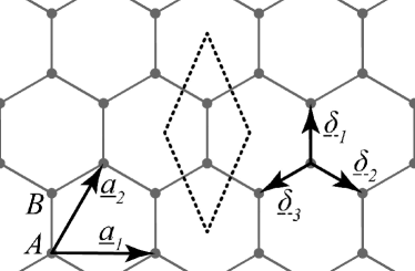
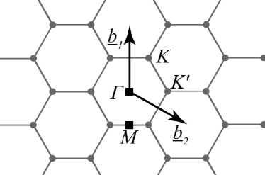
Figure 1: Left: Graphene with lattice vectors $\underline{a}_{1/2}$, translation vectors $\underline{\delta}_{i}$ and unit cell (dashed lines). Right: Reciprocal lattice with basis vectors $\underline{b}_{1/2}$, symmetry points $\underline{\Gamma}$, $\underline{K}$, $\underline{K}^{\prime}$, $\underline{M}$ and first Brillouin zone (hexagon).

Review of graphene.– The graphene (or honeycomb) lattice is bipartite with two triangular sublattices, labeled A and B. The position of a cell in the lattice is denoted by $\underline{R}=\alpha\underline{a}_{1}+\beta\underline{a}_{2}$ where $\alpha$ and $\beta$ are integers and $\underline{a}_{1(2)}$ are basis vectors of the lattice (see Fig. 1). States on the two sites within one cell will be denoted by $|R\rangle^{A(B)}\equiv|\alpha,\beta\rangle^{A(B)}$. The corners of the Brillouin zone (see Fig. 1) are denoted $\underline{K}$ and $\underline{K}^{\prime}$ and the primitive cell contains two of these points.

The solution for the tight-binding Hamiltonian on graphene as described above is well-known CN09 ; WA11 and leads to the dispersion relation

$$\epsilon\left(\underline{k}\right)=\epsilon_{D}\pm$$ (2)

$$v\sqrt{1+4\cos^{2}\left(\frac{k_{x}a}{2}\right)+4\cos\left(\frac{k_{x}a}{2}\right)\cos\left(\frac{\sqrt{3}k_{y}a}{2}\right)}$$

depicted in Fig. 2 for an infinite graphene lattice. It is indeed linear near the Dirac points $\underline{K}\text{ and }\underline{K}^{\prime}$ at the energy $\epsilon_{D}$ where the conduction and valence bands meet. Around the Dirac points the dispersion relation $\epsilon(\underline{k})$ can be approximated by

$$\epsilon\left(\underline{k}\right)\approx\epsilon_{D}\pm va\frac{\sqrt{3}}{2}\sqrt{\delta k_{x}^{2}+\delta k_{y}^{2}}=\epsilon_{D}\pm va\frac{\sqrt{3}}{2}\left|\delta k\right|.$$ (3)

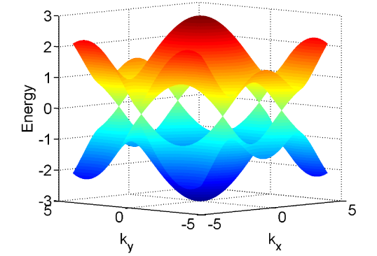
Figure 2: (Color online) Dispersion relation for infinite graphene sheet ($\epsilon_{D}=0$).

In the following, we will consider finite graphene lattices with periodic boundary conditions, i.e. $|\Psi\rangle=\sum_{\alpha=1}^{m}\sum_{\beta=1}^{n}\left(\psi_{\alpha,\beta}^{A}|\alpha,\beta\rangle^{A}+\psi_{\alpha,\beta}^{B}|\alpha,\beta\rangle^{B}\right)$ with $\psi^{A(B)}_{\alpha,\beta}=\psi^{A(B)}_{\alpha+m,\beta}=\psi^{A(B)}_{\alpha,\beta+n}$. This simplifies the analysis allowing us to focus on the relevant features of the search by avoiding boundary effects. The general description does not change for other boundary conditions, the localization amplitude on the marked site, however, becomes site dependent in a non-trivial way. Understanding this dependency is not essential in the context of this paper.

We denote $\underline{S}=m\underline{a}_{1}+n\underline{a}_{2}$ the vector describing the spatial dimensions of the lattice. Using Bloch’s theorem Kit05 , the momentum is quantized as

$$k_{x}=\frac{2\pi p}{ma}\hskip 14.22636ptk_{y}=\frac{1}{\sqrt{3}}\left(\frac{4\pi q}{na}-k_{x}\right)$$ (4)

where $p\in\left\{0,1,\ldots m-1\right\},q\in\left\{0,1,\ldots n-1\right\}$ and the spectrum (2) becomes discrete. In what follows, for simplicity, we have assumed that our lattice is square in the number of cells, that is, that $m=n=\sqrt{\frac{N}{2}}$. Four-fold degenerate states with energy $\epsilon_{D}$ and wave numbers exactly on the Dirac points $\underline{K}\text{ and }\underline{K}^{\prime}$ exist if $m$ and $n$ are some multiples of 3. We assume this in the following for simplicity. In the general case, one needs to consider the states closest to the Dirac energy which gives a more complex theoretical analysis while essential signatures do not change.

Quantum search.– Setting up a continuous-time search by changing the on-site energy of the marked site as done in Childs and Goldstone (2004) does not work for graphene. Using the ground state as the starting state fails for the same reason as it fails for rectangular lattices in $d=2$ or $3$ as the dispersion relation is quadratic near the ground state, see Fig. 2. Alternatively, moving the search to the Dirac point implies constructing an avoided crossing between a localized perturber state and a Dirac state. As the Dirac energy coincides with the on-site energy $\epsilon_{D}$, this leads to the condition, that the on-site energy perturbation must vanish at the crossing, which brings us back to the unperturbed lattice.

We therefore mark a given site by changing the hopping potentials between the site and its nearest neighbors. Focusing on a symmetric choice of the perturbation and setting $\epsilon_{D}=0$ for convenience, we obtain the (search-) Hamiltonian

$${\bf H}_{\gamma}=-\gamma{\bf A}+{\bf W}.$$ (5)

Here, ${\bf W}$ denotes the perturbation changing the hopping potential to and from the marked site $(\alpha_{0},\beta_{0})^{A}$ which has been chosen to be on the $A$ lattice, that is,

$${\bf W}=\sqrt{3}\left|\alpha_{0},\beta_{0}\right\rangle^{A}\left\langle\ell\right|+\sqrt{3}\left|\ell\right\rangle\left\langle\alpha_{0},\beta_{0}\right|^{A}.$$ (6)

The state $\left|\ell\right\rangle$ denotes the symmetric superposition of the three neighbors of the marked site, that is,

$$\left|\ell\right\rangle=\frac{1}{\sqrt{3}}\left(\left|\alpha_{0},\beta_{0}\right\rangle^{B}+\left|\alpha_{0},\beta_{0}-1\right\rangle^{B}+\left|\alpha_{0}+1,\beta_{0}-1\right\rangle^{B}\right).$$ (7)

At $\gamma=1$, the perturbation corresponds to a hopping potential $v=0$ between the site $(\alpha_{0},\beta_{0})^{A}$ and its neighbors, effectively removing the site from the lattice. It is this perturbation strength which is important in the following. Experimentally, such a perturbation is similar to graphene lattices with atomic vacancies as they occur naturally in the production process Meyer et al (2008); in microwave analogs of graphene as discussed in Kuhl et al (2010), this can be realized by removing single sites from the lattice.

The effect of marking (or perturbing) the graphene Hamiltonian can be seen numerically in the parametric behavior of the spectrum of ${\bf H}_{\gamma}$ as a function of $\gamma$, see Fig. 3 for the case $n=m=12$. Note that $\bf W$ is a rank two perturbation which creates two perturber states. These states start to interact with the spectrum of the unperturbed graphene lattice from $\gamma\approx 0.5$ onwards working their way through to a central avoided crossing at $\gamma=1,E=0$. Below we will show, how the avoided crossing can be used for searching; note, that the parameter dependence of the avoided crossing ($\gamma=1$) is evident from the tight-binding Hamiltonian $H$ in (5). In a realistic set-up, the perturbation needs to be fine-tuned in general to be in resonance with an eigenstate of the (unperturbed) system near the Dirac point.

At the avoided crossing there are altogether six states close to the Dirac energy: the two perturber states and the four degenerate Dirac states

$$\left|K\right\rangle^{A(B)}= \sqrt{\frac{2}{N}}\sum_{\alpha,\beta}e^{i\frac{2\pi}{3}\left(\alpha+2\beta+2\sigma\right)}\left|\alpha,\beta\right\rangle^{A(B)}$$

$$\left|K^{\prime}\right\rangle^{A(B)}= \sqrt{\frac{2}{N}}\sum_{\alpha,\beta}e^{i\frac{2\pi}{3}\left(2\alpha+\beta\right)}\left|\alpha,\beta\right\rangle^{A(B)}$$ (8)

where $\sigma=1$ ($\sigma=0$) for states on the B (A) lattice and $N=2nm$ is the number of sites in the lattice. One finds directly ${\bf W}\left|K\right\rangle^{B}={\bf W}\left|K^{\prime}\right\rangle^{B}=0$, that is, Dirac states on the B lattice do not interact with an A-type perturbation for all $\gamma$. Furthermore, at $\gamma=1$, the marked state $\left|\alpha_{0},\beta_{0}\right\rangle^{A}$ is an eigenvector of ${\bf H}_{\gamma=1}$ with eigenvalue $E=0$ - the marked site is disconnected from the lattice.

\begin{overpic}[width=455.3023pt]{12x12_3p_spectrum_colour} \put(54.25,26.75){\framebox{\includegraphics[width=160.43727pt]{3bond_gap_scale}}} \end{overpic}

Figure 3: Spectrum ${\bf H}_{\gamma}$ in Eq. 5 as a function of $\gamma$ for a $12\times 12$ cell torus ($N=288$). The spectrum is symmetric around $\epsilon_{D}=0$. Inset: Scaling of the gap $\Delta=\tilde{E}_{+}-\tilde{E}_{-}$ (dots) and curves $c_{1}/\sqrt{N}$ (solid blue), $c_{2}/\sqrt{N\log N}$ (dashed red) for comparison.

Thus, the avoided crossing involves only the two Dirac states $\left|K\right\rangle^{A}$, $\left|K^{\prime}\right\rangle^{A}$ and one perturber state $\left|\tilde{\ell}\right\rangle$. Neglecting the interaction of the perturbation with the rest of the spectrum at the avoided crossing, we set $\left|\tilde{\ell}\right\rangle\approx\left|\ell\right\rangle$ (see (7)) and use this to reduce the full Hamiltonian locally in terms of the $3$-dimensional basis $\{\left|K\right\rangle^{A},\left|K^{\prime}\right\rangle^{A},\left|\ell\right\rangle\}$. The reduced Hamiltonian takes the form

$$\tilde{\bf H}=\sqrt{\frac{6}{N}}\begin{bmatrix}0&0&e^{-i\frac{2\pi}{3}\left(\alpha_{o}+2\beta_{o}\right)}\\ 0&0&e^{-i\frac{2\pi}{3}\left(2\alpha_{o}+\beta_{o}\right)}\\ e^{i\frac{2\pi}{3}\left(\alpha_{o}+2\beta_{o}\right)}&e^{i\frac{2\pi}{3}\left(2\alpha_{o}+\beta_{o}\right)}&0\end{bmatrix}$$ (9)

with eigenvalues $\tilde{E}_{\pm}=\pm 2\sqrt{\frac{3}{N}},\tilde{E}_{0}=0$, and eigenvectors

$$\left|\tilde{\psi}_{\pm}\right\rangle =\frac{1}{2}\left(e^{-i\frac{2\pi}{3}\left(\alpha_{o}+2\beta_{o}\right)}\left|K\right\rangle^{A}+e^{-i\frac{2\pi}{3}\left(2\alpha_{o}+\beta_{o}\right)}\left|K^{\prime}\right\rangle^{A}\pm\sqrt{2}\left|\ell\right\rangle\right)$$ (10)

$$\left|\tilde{\psi}_{0}\right\rangle =\frac{1}{\sqrt{2}}\left(e^{-i\frac{2\pi}{3}\left(\alpha_{o}+2\beta_{o}\right)}\left|K\right\rangle^{A}-e^{-i\frac{2\pi}{3}\left(2\alpha_{o}+\beta_{o}\right)}\left|K^{\prime}\right\rangle^{A}\right).$$ (11)

For searching the marked site $(\alpha_{0},\beta_{0})^{A}$, the system is initialized in a delocalized starting state involving a superposition of Dirac states. This state will then rotate into a state localized on the neighbors of the marked site. The search is initialized in the optimal starting state

$$\left|s\right\rangle = \frac{1}{\sqrt{2}}\left(\left|\tilde{\psi}_{+}\right\rangle+\left|\tilde{\psi}_{-}\right\rangle\right)$$

$$= \frac{e^{-i\frac{2\pi}{3}\left(\alpha_{0}+2\beta_{0}\right)}}{\sqrt{2}}\left(\left|K\right\rangle^{A}+e^{-i\frac{2\pi}{3}\left(\alpha_{0}-\beta_{0}\right)}\left|K^{\prime}\right\rangle^{A}\right)$$

which still depends on the perturbed site. Lack of knowledge of $\left(\alpha_{0},\beta_{0}\right)$ leads, however, only to an $N$ independent overhead, see the discussion below. Letting $\left|s\right\rangle$ evolve in time with the reduced Hamiltonian (9) we obtain

$$\left|\psi\left(t\right)\right\rangle =e^{-i\tilde{\bf H}t}\left|s\right\rangle=\frac{1}{\sqrt{2}}{\left(e^{-i\tilde{E}_{+}t}\left|\tilde{\psi}_{+}\right\rangle+e^{-i\tilde{E}_{-}t}\left|\tilde{\psi}_{-}\right\rangle\right)}$$

$${=\cos\left(\tilde{E}_{+}t\right)\left|s\right\rangle-i\sin\left(\tilde{E}_{+}t\right)\left|\ell\right\rangle},$$ (13)

that is, the system rotates from $\left|s\right\rangle$ to $\left|\ell\right\rangle$ in time $t=\frac{\pi}{4}\sqrt{\frac{N}{3}}$. We find a $\sqrt{N}$ speed-up for the search on graphene. This, together with the linear dispersion relation near the Dirac point, where the spacing between successive eigenenergies scales like $O(1/\sqrt{N})$, makes the search on this 2D lattice possible. In contrast to the algorithms described in Childs and Goldstone (2004, 2004), the system localizes here on the neighbors of the marked site, the marked site can be found by three additional direct queries. Furthermore, the initial starting state is not the uniform state here, but the state $\left|s\right\rangle$ in (Quantum search on graphene lattices). To construct this initial state uniquely requires some information about the site that is being searched for. Without this knowledge, one has three possible optimal initial states for an A-type perturbation as can be seen from Eqn. (Quantum search on graphene lattices). The same applies for marking a B-type site, so in total there are six possible optimal starting states. As these states are not orthogonal, this increases the number of runs for a successful search by a factor of 4. The additional overhead is independent of N, and thus does not alter the scaling with system size. In an experiment one may have little control about how the system is excited at the Dirac energy, so the initial state will be in a more or less arbitrary superposition of all four Dirac states. The search is then not optimal but runs with a success probability that is, on average, again reduced by a factor $1/4$.

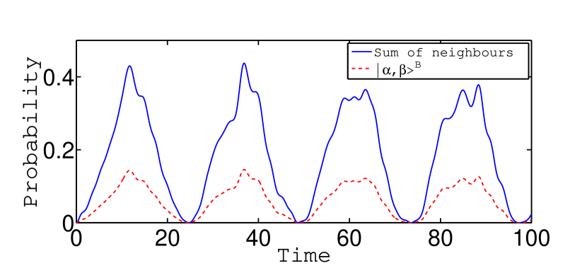
Figure 4: Search on $12\times 12$ cell graphene lattice with starting state $\left|s\right\rangle$. For tori with $m=n$ the dynamics at each neighboring site is the same so only one is shown.

Fig. 4 shows a numerically obtained quantum search initialized in $\left|s\right\rangle$ and evolving under the full search Hamiltonian. As expected from the analysis on the reduced Hamiltonian, the state localizes on the three neighboring sites with a probability of about 45% which is two orders of magnitude larger than the average probability $100/N$, here roughly 0.5%. The search does not reach 100% due to the fact that the actual localized state $|\tilde{\ell}\rangle$ extends beyond the nearest neighbors of the marked site, so $\langle{\tilde{\ell}}|{\ell}\rangle=O(1)<1$.

Our reduced model neglects contributions from the rest of the spectrum; like for other discrete and continuous time walks at the critical dimension FG98 ; Ambainis et al. (2005); ADMP10 ; Childs and Goldstone (2004, 2004), these contributions give $\ln N$ corrections (such as the $O\left(1/\sqrt{N\ln\left(N\right)}\right)$ scaling of the gap at the avoided crossing shown in the inset of Fig. 3). These logarithmic corrections have been derived in the appendix by going beyond the reduced three-state model, see also Childs and Goldstone (2004). The relevant exact eigenenergies $E_{+}=-E_{-}$ at the avoided crossing satisfy the resolvent condition

$$F\left(E_{\pm}\right)=\frac{\sqrt{3}}{N}\sum_{\underline{k}}\left[\frac{1}{E_{\pm}-\epsilon\left(\underline{k}\right)}+\frac{1}{E_{\pm}+\epsilon\left(\underline{k}\right)}\right]=0\,,$$ (14)

with $\epsilon(k)>0$ the eigenenergies of the unperturbed system at quasi-momenta $k$ given in (4). Expanding $F(E_{+})=4\sqrt{3}/(NE_{+})-\sum_{n=1}^{\infty}I_{2n}E_{+}^{2n-1}$, one finds $I_{2}=O(\mathrm{ln}N)$ and $I_{2k}=O(N^{k-1})$ for $k\geq 2$, see the appendix for details. The scaling of the gap follows then directly. The localization time scales inversely proportional to the gap, that is, $T=O\left(\sqrt{N\ln\left(N\right)}\right)$; one also obtains that the return amplitude drops like $O\left(1/\sqrt{\ln N}\right)$.

We note in passing that our search algorithm can - like all quantum searches - be used for quantum communication and state transfer. Following Hein and Tanner (2009b), our continuous time search can be used to send signals between different sites by adding an additional perturbation to the lattice. The quantum system is then initialized in a state localized on one of the perturbed sites and the system oscillates between states localized on the perturbations. We find that the mechanism works best when both perturbations are on the same sublattice. Due to the nature of the coupling between the A and B sublattice and the fact that the localized perturber states live (mostly) on one sublattice, signal propagation between perturbations on different sublattices takes place over a much longer timescale.

Discussion.– Continuous-time quantum search can be performed effectively on a 2D lattice without internal degrees of freedom by running the search at the Dirac point in graphene. We find that our search succeeds in time $T=O\left(\sqrt{N\ln\left(N\right)}\right)$ with probability $O\left(1/\ln N\right)$. This is the same time complexity found in Ambainis et al. (2005); ADMP10 for discrete-time and in Childs and Goldstone (2004) for continuous-time searches. To boost the probability to $O\left(1\right)$, $O\left(\ln N\right)$ repetitions are required giving a total time $T=O\left(\sqrt{N}\ln^{\frac{3}{2}}N\right)$. Amplification methods Grover (1997); Tulsi (2008); Potocek et al (2009) may be used to reduce the total search time further.

For simplicity of the analysis, we have focused here on perturbations which alter the hopping potential to all three nearest-neighbors symmetrically. Efficient search algorithms can also be obtained using other types of perturbations such as a single-bond perturbation or perturbing the lattice by adding additional sites. In all cases, it is important to fine-tune the system parameters in order to operate at an avoided crossing near the Dirac point. Given the importance of graphene as a nano-material, our findings point towards applications in directed signal transfer, state reconstruction or sensitive switching. This opens up the possibility of a completely new type of electronic engineering using single atoms as building blocks of electronic devices.

Appendix A Supplementary notes - Quantum search on graphene lattices

We present here supplementary notes related to the article Quantum search on graphene lattices. There, we proposed an implementation of an efficient continuous-time quantum search on a two-dimensional graphene lattice. The notes here provide additional details - not presented in the main text - on the scaling relation of the search time and the success probability. We derive in particular the $\log N$ correction terms.

The search dynamics is defined through a tight-binding Hamiltonian $H$ consisting of the Hamiltonian of the unperturbed (finite) graphene lattice, $H_{0}$, and a perturbation term changing the hopping potential between a single marked site $\left|\alpha_{o},\beta_{o}\right\rangle$ and its three neighbors. The perturbation has the effect of decoupling the marked site from its neighbors. The Hamiltonian is of the form

$$H=H_{0}+\sqrt{3}\left|\alpha_{o},\beta_{o}\right\rangle\left\langle\ell\right|+\sqrt{3}\left|\ell\right\rangle\left\langle\alpha_{o},\beta_{o}\right|$$ (15)

and we assume periodic boundary conditions on the unperturbed graphene Hamiltonian $H_{0}$, see the main text for details. Here, $\left|\ell\right\rangle$ is a uniform superposition of the three neighboring vertices adjacent to $\left|\alpha_{o},\beta_{o}\right\rangle$. We derive in what follows the search time $t=T$, that is, the time at which the amplitude at $\left|\ell\right\rangle$ reaches a maximum. The amplitude squared is interpreted as the success probability for the search to succeed. The amplitude is determined by evaluating

$$\left\langle\ell\right|e^{-iHT}\left|start\right\rangle=\sum_{\left|\psi_{a}\right\rangle}\left\langle\ell\vphantom{\psi_{a}}\right|\left.\psi_{a}\vphantom{\ell}\right\rangle\left\langle\psi_{a}\vphantom{start}\right|\left.start\vphantom{\psi_{a}}\right\rangle e^{-iE_{a}T},$$ (16)

with $\left|\psi_{a}\right\rangle$, $E_{a}$, the eigenstates and eigenenergies of the perturbed lattice. Note that $\left|\alpha_{o},\beta_{o}\right\rangle$ is itself an eigenstate with $H\left|\alpha_{o},\beta_{o}\right\rangle=0$ and $\left\langle\ell\vphantom{\alpha_{o},\beta_{o}}\right|\left.\alpha_{o},\beta_{o}\vphantom{\ell}\right\rangle=0$, so that it does not contribute to the sum (16). Without loss of generality, we choose our initial state on the A sublattice of graphene, that is

$$\left|start\right\rangle=\frac{1}{\sqrt{2}}\left(\left|A_{\underline{K}}\right\rangle+\left|A_{\underline{K}^{\prime}}\right\rangle\right)$$ (17)

with $\left|A_{\underline{K}}\right\rangle,\left|A_{\underline{K}^{\prime}}\right\rangle$ being degenerate eigenenergies of the unperturbed lattice at the Dirac energy and on the A-lattice. (If the perturbation is on the B-lattice, the search is not successful and we repeat the search on the B sublattice). In these notes, we will justify our simple reduced model in the main text showing that our algorithm effectively takes place in a two-dimensional subspace of the full Hilbert-space spanned by combinations of the energy-states near the Dirac point and a localized perturber state. Our analysis follows the treatment in Ref. [S1] adjusted to include symmetry properties of graphene around the Dirac point.

For any eigenstate $\left|\psi_{a}\right\rangle$ of the perturbed system such that the corresponding eigenenergy $E_{a}$ is not in the spectrum of $H_{0}$ we may rewrite the perturbed eigenequation in the form

$$\left|\psi_{a}\right\rangle=\frac{\sqrt{3R_{a}}}{E_{a}-H_{0}}\left|\alpha_{o},\beta_{o}\right\rangle,$$ (18)

where $\sqrt{R_{a}}=\left\langle\ell\vphantom{\psi_{a}}\right|\left.\psi_{a}\vphantom{\ell}\right\rangle$ (where we chosen the phase of $\left|\psi_{a}\right\rangle$ such that$\left\langle\ell\vphantom{\psi_{a}}\right|\left.\psi_{a}\vphantom{\ell}\right\rangle\geq 0$).
If $E_{a}$ is in the spectrum of $H_{0}$ then $\sqrt{R_{a}}=0$. This is trivial for the state $\left|\psi_{a}\right\rangle=\left|\alpha_{o},\beta_{o}\right\rangle$ – otherwise it can be shown as follows. Let $\left|\psi_{a}^{0}\right\rangle$ be an unperturbed eigenvector such that $H_{0}\left|\psi_{a}^{0}\right\rangle=E_{a}\left|\psi_{a}^{0}\right\rangle$. Projecting the eigenvalue equation $H\left|\psi_{a}\right\rangle=E_{a}\left|\psi_{a}\right\rangle$ onto $\left|\psi_{a}^{0}\right\rangle$ yields $\left\langle\psi_{a}^{0}\vphantom{\ell}\right|\left.\ell\vphantom{\psi_{a}^{0}}\right\rangle\left\langle\alpha_{o},\beta_{o}\vphantom{\psi_{a}}\right|\left.\psi_{a}\vphantom{\alpha_{o},\beta_{o}}\right\rangle+\left\langle\psi_{a}^{0}\vphantom{\alpha_{o},\beta_{o}}\right|\left.\alpha_{o},\beta_{o}\vphantom{\psi_{a}^{0}}\right\rangle\left\langle\ell\vphantom{\psi_{a}}\right|\left.\psi_{a}\vphantom{\ell}\right\rangle=0$. Clearly, $\left\langle\alpha_{o},\beta_{o}\vphantom{\psi_{a}}\right|\left.\psi_{a}\vphantom{\alpha_{o},\beta_{o}}\right\rangle=0$; in addition for a given $E_{a}$, we can always find at least one corresponding $\left|\psi_{a}^{0}\right\rangle$ such that $\left\langle\psi_{a}^{0}\vphantom{\alpha_{o},\beta_{o}}\right|\left.\alpha_{o},\beta_{o}\vphantom{\psi_{a}^{0}}\right\rangle\neq 0$. From that it follows that $\left\langle\ell\vphantom{\psi_{a}}\right|\left.\psi_{a}\vphantom{\ell}\right\rangle=0\equiv R_{a}^{2}$, which is what we wanted to show. Note that due to high degeneracies in the unperturbed system and due to the fact, that the perturbation is of rank two, one will have many states whose eigenenergies do not change under the perturbation and for which (18) is a priori not well defined. The property $R_{a}=0$ allows us to remove these states from all sums that involve $(E_{a}-H_{0})^{-1}$.

Let us now use (18) to derive a condition for an energy $E_{a}\neq 0$ to be a perturbed eigenenergy of $H$ – perturbed eigenenergy here implies that it is not in the spectrum of $H_{0}$. As $\left|\alpha_{o},\beta_{o}\right\rangle$ is a known eigenstate of the perturbed lattice, we have $\left\langle\alpha_{o},\beta_{o}\vphantom{\psi_{a}}\right|\left.\psi_{a}\vphantom{\alpha_{o},\beta_{o}}\right\rangle=0$ and thus (18) implies

$$\sqrt{3R_{a}}\left\langle\alpha_{o},\beta_{o}\right|\left(E_{a}-H_{0}\right)^{-1}\left|\alpha_{o},\beta_{o}\right\rangle=0\,.$$ (19)

Expressing $\left\langle\alpha_{0},\beta_{0}\right|$ in terms of the eigenstates of the unperturbed Hamiltonian $H_{0}$, we may write this as a quantization condition

$$\begin{split}F\left(E_{a}\right)=&0\\ F\left(E\right)=&\frac{\sqrt{3}}{N}\sum_{\underline{k}}\left[\frac{1}{E-\epsilon\left(\underline{k}\right)}+\frac{1}{E+\epsilon\left(\underline{k}\right)}\right].\end{split}$$ (20)

Here, $N$, is the total number of sites and $\epsilon\left(\underline{k}\right)$ are the positive eigenenergies of the unperturbed Hamiltonian $H_{0}$. (Note that the spectrum of $H_{0}$ as well as $H$ is symmetric around $E=0$. This constitutes the main difference to the treatment considered in [S1]. )
We may choose $\left|\psi_{a}\right\rangle$ to be normalized $\left\langle\psi_{a}\vphantom{\psi_{a}}\right|\left.\psi_{a}\vphantom{\psi_{a}}\right\rangle=1$ – (18) then implies

$$3R_{a}\left\langle\alpha_{o},\beta_{o}\right|\left(E_{a}-H_{0}\right)^{-2}\left|\alpha_{o},\beta_{o}\right\rangle=1,$$ (21)

which allows $R_{a}$ to be rewritten as

$$R_{a}=\frac{1}{\sqrt{3}|{F^{\prime}\left(E_{a}\right)}|}.$$ (22)

We may now rewrite the amplitude (16) in the form

$$\begin{split}\left\langle\ell\right|e^{-iHT}\left|start\right\rangle=&\sum_{a:R_{a}\neq 0}\sqrt{R_{a}}\left\langle\psi_{a}\vphantom{start}\right|\left.start\vphantom{\psi_{a}}\right\rangle e^{-iE_{a}T}\\ =&\left\langle\alpha_{o},\beta_{o}\vphantom{start}\right|\left.start\vphantom{\alpha_{o},\beta_{o}}\right\rangle\sum_{a}\frac{e^{-iE_{a}T}}{E_{a}|{F^{\prime}\left(E_{a}\right)}|}\,\end{split}$$ (23)

where we have used the adjoint of (18) and have removed the restrictions on the summation in the last line. This is no longer necessary as $|F^{\prime}(E_{a})|\to\infty$ when $E_{a}$ is in the unperturbed spectrum. In the main text, we show that by adding a perturbation which creates a localized state energetically close to the Dirac point one can construct an efficient search algorithm. Consequently, we concentrate on evaluating the time-evolution involving the eigenstates of the perturbed Hamiltonian closest to the Dirac point; we denote these states $\left|\psi_{\pm}\right\rangle$ in what follows. We estimate the corresponding eigenenergies, $E_{\pm}$ where $E_{+}=-E_{-}>0$ and we will focus on $E_{+}$ in the following. Using the sum in Eq. (20), we will also derive a leading order expression for $F^{\prime}\left(E_{+}\right)$. Separating out the contribution to $F\left(E_{+}\right)$ from the Dirac points where $\epsilon\left(\underline{K}\right)=\epsilon\left(\underline{K}^{\prime}\right)=0$, and expanding the remaining contribution to the sum in (20) at $E=0$, one obtains

$$F\left(E_{+}\right)=\frac{4\sqrt{3}}{NE_{+}}-\sum_{n=1}^{\infty}I_{2n}E_{+}^{2n-1}.$$ (24)

The sums $I_{n}$ are given by

$$I_{n}=\frac{\sqrt{3}}{N}\sum_{\underline{k}\neq\underline{K},\underline{K}^{\prime}}\left[\frac{1}{\left[\epsilon\left(\underline{k}\right)\right]^{n}}+\frac{1}{\left[-\epsilon\left(\underline{k}\right)\right]^{n}}\right]\,.$$ (25)

Due to the symmetry of the unperturbed spectrum only those $I_{n}$ with even $n$ are non-zero.

The non-vanishing $I_{2k}$ coefficients obey the following rigorous estimates

$$I_{2}= O\left(\ln N\right),$$ (26)

$$\lim_{N\to\infty}\frac{I_{2k}}{N^{k-1}}= 4\sqrt{3}\left(Z_{2}(S_{\underline{K}},k)+Z_{2}(S_{\underline{K}^{\prime}},k)\right)$$

for $$k\geq 2$$, (27)

where the estimate (26) is sharp ($I_{2}$ is logarithmically bounded from above and below) and $Z_{2}(S,x)$ is the Epstein zeta-function

$$Z_{2}(S,x)=\frac{1}{2}\sum_{(p,q)\in\mathbb{Z}^{2}\backslash(0,0)}\left(S_{11}p^{2}+2S_{12}pq+S_{22}q^{2}\right)^{-x}$$ (28)

for a real positive definite real symmetric $2\times 2$ matrix $S$ [S2]. The matrices

$$S_{\underline{K}}=S_{\underline{K}^{\prime}}=4\pi^{2}\begin{pmatrix}2&-1\\ -1&2\end{pmatrix}$$ (29)

describe the spectrum close to the Dirac points. The linear dispersion behaviour near the Dirac points $K$ and $K^{\prime}$ is the same and so are the matrices $S_{\underline{K}}$ and $S_{\underline{K}^{\prime}}$.
Before moving on let us derive the estimates (26) and (27). It is clear that the dominant contributions come from the vicinity of the Dirac points. Approximating the spectrum close to the Dirac points one has

$$\begin{split}I_{2k}=&2\sqrt{3}N^{k-1}\left[\sum_{(p,q)\in L}\frac{1}{\left(S_{\underline{K},11}p^{2}+2S_{\underline{K},12}pq+S_{\underline{K},22}q^{2}\right)^{k}}+\right.\\ &\left.\sum_{(p,q)\in L}\frac{1}{\left(S_{\underline{K^{\prime}},11}p^{2}+2S_{\underline{K^{\prime}},12}pq+S_{\underline{K^{\prime}},22}q^{2}\right)^{k}}\right]+O(1)\ .\end{split}$$ (30)

Here the sums over integers $p$ and $q$ is over a rectangular region $L$ of the lattice $\mathbb{Z}^{2}$ which is centered at $(0,0)$ and has side lengths proportional to $\sqrt{N}$ – the center $(0,0)$, corresponding to the relevant Dirac point, is omitted from the sum. For $k>1$ the corresponding sums converge which proves (27).
For $k=1$ we will establish constant $C_{1}$ and $C_{2}$ such that

$$C_{1}\ln N<\sum_{(p,q)\in L}\frac{1}{S_{\underline{K},11}p^{2}+2S_{\underline{K},12}pq+S_{\underline{K},22}q^{2}}<C_{2}\ln N$$ (31)

which then directly leads to (26). To establish $C_{1}$ note that because each term in the sum (31) is positive its value decreases by restricting it to a square region $-a_{1}\sqrt{N}\leq p\leq a_{1}\sqrt{N}$, $-a_{1}\sqrt{N}\leq q\leq a_{1}\sqrt{N}$ which is completely contained in $L$. Up to an error of order one the sum over a square region can in turn be written as a sum over eight terms of the form

$$\sum_{p=1}^{a_{1}\sqrt{N}}\sum_{q=1}^{p}\frac{1}{S_{\underline{K},11}p^{2}\pm 2S_{\underline{K},12}pq+S_{\underline{K},22}q^{2}}\ .$$ (32)

For fixed $p$ we can find $q_{\mathrm{max}}$ such that

$$\sum_{q=1}^{p}\frac{1}{S_{\underline{K},11}p^{2}\pm 2S_{\underline{K},12}pq+S_{\underline{K},22}q^{2}}>\\ \frac{p}{S_{\underline{K},11}p^{2}\pm 2S_{\underline{K},12}pq_{\mathrm{max}}+S_{\underline{K},22}q_{\mathrm{max}}^{2}}\ .$$ (33)

We may choose $q_{\mathrm{max}}=b_{1}p$ for some constant $b_{1}\geq 0$, so

$$\sum_{p=1}^{a_{1}\sqrt{N}}\sum_{q=1}^{p}\frac{1}{S_{\underline{K},11}p^{2}\pm 2S_{\underline{K},12}pq+S_{\underline{K},22}q^{2}}>c\sum_{p=1}^{\sqrt{N}}\frac{1}{p}$$ (34)

which diverges as $\ln N$.

Establishing $C_{2}$ and the corresponding logarithmic bound from above follows the same line by first extending the sum to a square of side length $2a_{2}\sqrt{N}$ that completely contains $L$ and then establishing

$$\sum_{q=1}^{p}\frac{1}{S_{\underline{K},11}p^{2}\pm 2S_{\underline{K},12}pq+S_{\underline{K},22}q^{2}}<\\ \frac{p}{S_{\underline{K},11}p^{2}\pm 2S_{\underline{K},12}pq_{\mathrm{min}}+S_{\underline{K},22}q_{\mathrm{min}}^{2}}\$$ (35)

with $q_{min}=b_{2}p$.
Let us note in passing that estimates based on Poisson summation reveal more detail, i.e.

$$I_{2}= A\ln N+O(1),$$ (36)

$$I_{2k}= 2\sqrt{3}N^{k-1}\left(Z_{2}(S_{\underline{K}},k)+Z_{2}(S_{\underline{K}^{\prime}},k)\right)+$$

$$\quad+O(N^{k-2})\qquad\qquad\qquad\text{for $k\geq 2$,}$$ (37)

where $A>0$ is a constant. A rigorous treatment of the $O(1)$ estimate is more involved, however. In fact, (26)and (27) are sufficient in the context of this paper.

We note that each term in $Z_{2}\left(S_{\underline{K}},k\right)$ is smaller than the corresponding term in $Z_{2}\left(S_{\underline{K}},2\right)$ for $k>2$, and so it follows that $Z_{2}(S_{\underline{K}},k)<Z_{2}(S_{\underline{K}},2)$ for $k>2$. This property of the Epstein zeta function and the estimate (27) imply $\sum_{n=2}^{\infty}I_{2n}E_{+}^{2n-1}<\frac{C}{NE_{+}}\sum_{n=2}^{\infty}(NE_{+}^{2})^{n}$ i.e. the infinite sum in (24) converges for $E_{+}<1/\sqrt{N}$.

Let us now show that one indeed finds a solution of $F(E_{+})=0$ using the expansion (24) inside the convergence radius. We start with the estimate that is obtained by truncating the sum in (24) at $n=1$, i.e. $\frac{4\sqrt{3}}{NE_{+}}-I_{2}E_{+}=0$. This estimate gives $E_{+}^{2}\approx\frac{4\sqrt{3}}{NI_{2}}$ – for sufficiently large $N$ this is in the radius of convergence of the complete expansion (24). We will now show rigorously that this estimate gives the leading order correctly. First of all, the estimate implies that a zero inside the radius of convergence exists. Moreover since $I_{2n}>0$ all terms of (24) that have been neglected in the estimate enter with the same sign. So the true value $E_{+}>0$ has to be smaller than the estimate, which we write as

$$E_{+}^{2}=\frac{4\sqrt{3}}{NI_{2}}-\Delta>0$$ (38)

with $\Delta>0$. We will show rigorously that $\Delta/E_{+}\to 0$ as $N\to\infty$. Indeed one may rewrite $F(E_{+})=0$ in the form

$$\frac{4\sqrt{3}}{N}-I_{2}E_{+}^{2}= \sum_{n=2}^{\infty}I_{2n}E_{+}^{2n}\qquad\quad$$ (39)

$$\Rightarrow I_{2}\Delta= \sum_{n=2}^{\infty}I_{2n}E_{+}^{2n}.$$ (40)

Following the same arguments as used above for the calculation of the convergence radius and using the already established fact that $E_{+}$ is inside the convergence radius for sufficiently large $N$ we get the following inequality

$$0<NI_{2}\Delta < C\sum_{n=2}^{\infty}(NE_{+}^{2})^{n}$$

$$= \frac{CN^{2}E_{+}^{4}}{1-NE_{+}^{2}}=O(I_{2}^{-2}).$$

So $\Delta=O(I_{2}^{-3}N^{-1})=O\left((\ln N)^{-3}N^{-1}\right)$, or $\Delta/E_{+}=O\left((\ln N)^{-5/2}N^{-1/2}\right)$. We thus obtain

$$E_{+}^{2}=\frac{4\sqrt{3}}{NI_{2}}\left(1-O({(\ln N)^{-2}})\right),$$ (41)

and analogously

$$F^{\prime}\left(E_{\pm}\right)=-2I_{2}+O\left(\frac{1}{\ln N}\right).$$ (42)

This allows us to show that only two states have an overlap $O(1)$ with the starting state and are thus the relevant states to be considered in the time-evolution of the algorithm. Using the definitions of $\left|\psi_{a}\right\rangle$ and $R_{a}$ in Eqs. (18) and (22), the inner product of the starting state and the perturbed eigenvectors can be expressed as

$$\left\langle start\vphantom{\psi_{a}}\right|\left.\psi_{a}\vphantom{start}\right\rangle=\frac{3^{\frac{1}{4}}}{E_{a}|F^{\prime}\left(E_{a}\right)|^{\frac{1}{2}}}\left\langle start\vphantom{\alpha_{o},\beta_{o}}\right|\left.\alpha_{o},\beta_{o}\vphantom{start}\right\rangle.$$ (43)

Applying our previous results for the states nearest to the Dirac point, we see that

$$|\left\langle start\vphantom{\psi_{\pm}}\right|\left.\psi_{\pm}\vphantom{start}\right\rangle|\approx\frac{1}{\sqrt{2}}+O\left(\frac{1}{\ln^{2}N}\right).$$ (44)

Our starting state is thus a superposition of the perturbed eigenstates, $\left|\psi_{\pm}\right\rangle$, which also facilitate the search algorithm, see the main text. This now allows us to investigate the running time and success amplitude of the algorithm by looking at the time-evolution, that is,

$$\left|\left\langle\ell\right|e^{-iHt}\left|start\right\rangle\right|$$ (45)

$$\approx\left|\frac{1}{\sqrt{2}}\left(e^{-iE_{+}t}\left\langle\ell\vphantom{\psi_{+}}\right|\left.\psi_{+}\vphantom{\ell}\right\rangle-e^{iE_{+}t}\left\langle\ell\vphantom{\psi_{-}}\right|\left.\psi_{-}\vphantom{\ell}\right\rangle\right)\right|$$ (46)

$$=\frac{1}{3^{\frac{1}{4}}I_{2}^{\frac{1}{2}}}\left|\sin\left(E_{+}t\right)\right|$$ (47)

It is clear from our earlier results for $E_{\pm}$ and $I_{2}$ that our algorithm localizes on the neighbor state $\left|\ell\right\rangle$ in time $T=\frac{\pi}{2E_{+}}=O\left(\sqrt{N\ln N}\right)$ with probability amplitude $O\left(1/\sqrt{\ln N}\right)$.

[S1] Spatial search by quantum walk, Andrew M. Childs and Jeffrey Goldstone, Phys. Rev. A. 70:022314 (2004).

[S2] On Advanced Analytic Number Theory, C.L. Siegel, Tata Institute of Fundamental Research (1961).