Non-normalizable densities in strong anomalous diffusion: beyond the central limit theorem

Abstract

Strong anomalous diffusion, where $\langle|x(t)|^{q}\rangle\sim t^{q\nu(q)}$ with a nonlinear spectrum $\nu(q)\neq\mbox{const}$, is wide spread and has been found in various nonlinear dynamical systems and experiments on active transport in living cells. Using a stochastic approach we show how this phenomena is related to infinite covariant densities, i.e., the asymptotic states of these systems are described by non-normalizable distribution functions. Our work shows that the concept of infinite covariant densities plays an important role in the statistical description of open systems exhibiting multi-fractal anomalous diffusion, as it is complementary to the central limit theorem.

Consider particles diffusing in a medium with their total number conserved. Within a probabilistic approach the density $P(x,t)$ is normalized to unity $\int_{-\infty}^{\infty}P(x,t){\rm d}x=1$ for any time $t$. It follows naturally that the steady state of a system in equilibrium is normalized, e.g., the Boltzmann-Gibbs distribution which serves as the basis of statistical physics in thermal equilibrium. In contrast, infinite ergodic theory is a branch of mathematics that investigates dynamical systems whose invariant density is non-normalizable Aaronson ; Thaler . Current models characterized by non-normalized densities include intermittent maps KorabelPesin ; KorabelINF ; Akimotoprl and the momentum distribution of particles in optical lattice KesslerPRL ; LutzNature ; Holz . These systems attain equilibrium, i.e., the non-normalized densities is an extension of Boltzmann-Gibbs like states KesslerPRL ; LutzNature , and unfortunately we conclude that real-life applications of infinite ergodic theory are limited. Here we investigate unbounded systems which are not in equilibrium, inspired by infinite ergodic theory, we find that non-normalized covariant densities (defined below) play an important role in the description of anomalous diffusion. The potential applications of infinite covariant densities in real world experiments is shown to be vast. These uncommon densities provide a detailed description of the rare fluctuations in strong anomalous diffusion.

Strong anomalous diffusion deals with processes, with a long time $t$ asymptotic behavior, satisfying $\langle|x(t)|^{q}\rangle\sim t^{q\nu(q)}$, $q>0$, where $\nu(q)$ is not a constant Strong , in contrast with standard Brownian motion where $\nu(q)=1/2$. Such diffusion has been detected in a variety of processes: in the transport in two-dimensional incompressible velocity fields Strong , particle spreading in billiard systems Edelman ; Artuso ; Armstead ; Sanders ; Courbage , avalanche dynamics of sand pile models Sandpile , and in statistics of occupation times of renewal processes GL . Recent experiments on the active transport of polystyrene beads in living cells Naama , theoretical investigation of cold atoms in optical lattices DechantPRL and flows in porous media Anna further confirmed the generality of strong anomalous diffusion. Remarkably, in all these systems a piecewise-linear scaling, with $q\nu(q)\sim q$ below some critical value of $q$, and with $q\nu(q)=q-b$ above this critical value, was found. An analytical approach to this bilinear scaling, for deterministic chaotic dynamics was presented in Ref. Artuso . Such strong anomalous diffusion is an indication of the breakdown of mono-scaling theories which predict $P(x,t)\sim t^{-\nu}f(x/t^{\nu})$, e.g., normal diffusion where $f(\cdot)$ is Gaussian. In this Letter we explain how this breakdown is related to non-normalizable densities. By investigating a large class of stochastic processes, the so-called Lévy walks Shles ; Klafter ; Bouchaud ; Review , we demonstrate how these densities describe statistics of strong anomalous diffusion. Our work shows how infinite covariant densities are complementary to the Lévy-Gauss central limit theorem, which presents the mathematical foundation of diffusion phenomena.

The Lévy walk model Shles ; Klafter ; Bouchaud ; Review is a widely applicable process describing strong anomalous diffusion Andersen . To demonstrate the broad validity of our approach we consider two different classes of the model and four examples. In the velocity model ZK , a particle in one dimension starts on the origin $x=0$ at time $t=0$ and travels with velocity $v_{1}$, drawn from a probability density function (PDF) $F(v)$. The duration of the traveling event $\tau_{1}$ is drawn from the PDF $\psi(\tau)$. The process is then renewed, namely, a new velocity $v_{2}$ and flight duration $\tau_{2}$ are drawn from $F(v)$ and $\psi(\tau)$ respectively. The process continues in this manner until time $t$. The position of the particle is $x=\int_{0}^{t}v(t){\rm d}t$, as usual. In the jump model ZK ; KBS , a particle first waits on $x=0$ for time $\tau$, drawn from $\psi(\tau)$, and performs a jump with probability $1/2$ to a distance $x=v_{0}\tau$ or $x=-v_{0}\tau$, where $v_{0}=\mbox{const}$. The process is then renewed. For the velocity model we assume that $F(v)=F(-v)$ and that all the moments of $F(v)$ are finite. We will address three cases: (i) a two state velocity model, $F(v)=\left[\delta(v-v_{0})+\delta(v+v_{0})\right]/2$, (ii) a Gaussian and (iii) exponential velocity PDFs. The main ingredient of the Lévy walk model is the waiting time PDF of the power law form

$$\psi(\tau)\sim{A\over|\Gamma(-\alpha)|}\tau^{-(1+\alpha)}$$ (1)

with $1<\alpha<2$ and $A>0$. This choice of parameters insures that the average waiting time, $\langle\tau\rangle$, is finite but the variance of the waiting time is infinite. These types of random walks have been widely investigated and specific values of $\alpha$ have been recorded in several experiments Ott ; Solomon ; Hoog ; Wiersma ; Sims ; Jager ; Harris ; Sagi and calculated from first principle models KesBarPRL ; Zabu .

Montroll-Weiss equation. Let $P(x,t)$ be the PDF of the particle’s position at time $t$. The well known Montroll-Weiss equation ZK ; KBS gives the Fourier-Laplace transform of $P(x,t)$ for the velocity model Carry

$$P(k,u)={\overline{W}(k,u)\over 1-\overline{\psi}(k,u)},$$ (2)

where $\overline{\psi}(k,u)=\int_{0}^{\infty}\int_{-\infty}^{\infty}\exp(-u\tau+ikv\tau)F(v)\psi(\tau){\rm d}\tau{\rm d}v$ and similarly for $\overline{W}(k,u)$ with $W(t)=\int_{t}^{\infty}\psi(\tau){\rm d}\tau$. Here $W(t)$ is the persistence probability to reach $x$ in a single travelling event. Henceforth we use the convention that the variables in a function’s parenthesis, e.g., $P(x,t)$ or $P(k,u)$, define the space we are working in.

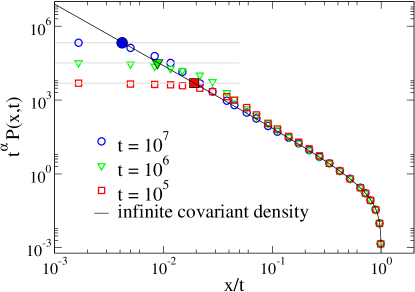
Figure 1: (color online) Rescaled PDFs $t^{\alpha}P(x,t)$ (open symbols) versus $x/t$ for the jump model with $\alpha=3/2,A=v_{0}=1$ remarkSim for three different times. The bold black line depicts the ICD of the process Eq. (11). Error bars are smaller then the size of the symbols. Big filled symbols indicate the locations of the crossover velocities $\overline{v}_{c}$ and horizontal lines are Lévy’s central limit theory for $t^{\alpha}P(x=0,t)$ (see the main text for more details).

The Fourier transform $P(k,t)$ is Taylor expanded

$$P(k,t)=1+\sum_{n=1}^{\infty}{(ik)^{n}\langle x^{n}(t)\rangle\over n!},$$ (3)

where the first term is the normalization $P(k=0,t)=1$. Using Eq. (2) we obtain the integer moments of the process in the long time limit. The $n$-th moment is obtained by differentiating $\langle x^{n}(u)\rangle=d^{n}P(k,u)/d(ik)^{n}|_{k=0}$ with $\psi(u)\sim 1-\langle\tau\rangle u+Au^{\alpha}$ and then by Laplace inversion. This is a standard procedure for $n=2$ Review and we use the Faá di Bruno formula Warren to obtain the exact asymptotic expressions for all the higher order moments. The even $n$-th moment of the two state velocity model is

$$\langle x^{n}(t)\rangle\sim{n\over(n-\alpha)(n+1-\alpha)}{A\over|\Gamma(1-\alpha)|\langle\tau\rangle}(v_{0})^{n}t^{n+1-\alpha},$$ (4)

while odd moments are zero, due to the symmetry of $F(v)$. The process exhibits super-diffusion $\langle x^{2}\rangle\sim t^{3-\alpha}$ because $1<\alpha<2$. We insert Eq. (4) in Eq. (3) and find

$$P_{A}(k,t)\sim 1+t^{1-\alpha}{A\over|\Gamma(1-\alpha)|\langle\tau\rangle}\tilde{f}_{\alpha}(ikv_{0}t),$$ (5)

where the subscript $A$ in $P_{A}(k,t)$ stands for the $t\to\infty$ asymptotics and

$$\tilde{f}_{\alpha}(iy)=\sum_{n=1}^{\infty}{(iy)^{2n}\over(2n-1)!(2n-\alpha)(2n+1-\alpha)}.$$ (6)

Summing this series we get

$$\tilde{f}_{\alpha}(iy)=y^{2}\left[{1\over 3-\alpha}\ _{1}F_{2}\left({3-\alpha\over 2};{3\over 2},{5-\alpha\over 2};{-y^{2}\over 4}\right)-{1\over 2-\alpha}\ _{1}F_{2}\left(1-{\alpha\over 2};{3\over 2},2-{\alpha\over 2};{-y^{2}\over 4}\right)\right]$$ (7)

where ${}_{1}F_{2}$ is a Hypergeometric function. Next we invert the asymptotic expression $P_{A}(k,t)$, Eq. (5), using the inverse Fourier transform and Eq. (7). Since we use the exact expressions for the long time behavior of the moments of the process, one may be tempted to believe that this procedure finally yields the long time limit of the normalized spreading packet $P(x,t)$. Indeed for normal transport, for example, when the waiting times are exponentially distributed, this procedure yields the familiar Gaussian distribution. Instead, for the two state Lévy walk model, we find

$$P_{A}(x,t)={1\over t^{\alpha}}{A\over 2v_{0}\langle\tau\rangle\left|\Gamma(1-\alpha)\right|}\left|{x\over v_{0}t}\right|^{-(1+\alpha)}\left[\alpha-\left(\alpha-1\right)\left|{x\over v_{0}t}\right|\right]\ \mbox{for}\ \ |x|<v_{0}t,\ \ x\neq 0,$$ (8)

while $P_{A}(x,t)=0$ for $|x|>v_{0}t$. Notice that in the vicinity of $x\to 0$ we find $P_{A}(x,t)\sim|x|^{-1-\alpha}$, therefore it is non-normalizable. Within our approach we first take the long time limit (in the calculation of the moments) and only then perform the inverse Fourier transform. These two mathematical operations do not commute, namely, the inverse Fourier transform of $P(k,t)$, for any finite $t$, yields a normalized density. Still as we proceed to show, the non-normalized state Eq. (8) describes statistical properties of the spreading packet of particles and hence physical reality.

Infinite covariant density. We now define the infinite covariant density (ICD) according to

$$\lim_{t\to\infty}t^{\alpha}P(x,t)=I_{\rm{cd}}(\overline{v})$$ (9)

where $\overline{v}\equiv{x/t}=\int_{0}^{t}v(t){\rm d}t/t$ is the $t\to\infty$ time averaged velocity of the particle. Since both $P(x,t)$ and $P_{A}(x,t)$ provide the asymptotic moments of the process, in the asymptotic regime Eqs. (8,9) give

$$I_{\rm{cd}}(\overline{v})=K_{\alpha}c_{\alpha}|\overline{v}|^{-(1+\alpha)}\left[1-{\alpha-1\over\alpha}{|\overline{v}|\over v_{0}}\right],$$ (10)

if $|\overline{v}|/v_{0}\leq 1$, otherwise $I_{\rm{cd}}(\overline{v})=0$, and $c_{\alpha}=\sin(\pi\alpha/2)\Gamma(1+\alpha)/\pi$, $K_{\alpha}=A\langle|v|^{\alpha}\rangle|\cos(\pi\alpha/2)|/\langle\tau\rangle$ with $\langle|v|^{\alpha}\rangle=\int_{-\infty}^{\infty}|v|^{\alpha}F(v){\rm d}v$. Here $K_{\alpha}$ is the anomalous diffusion constant, a measurable observable, soon to be discussed.

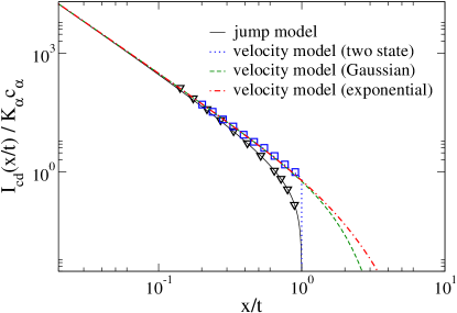
Figure 2: (color online) ICDs for different Lévy walk models, with $\alpha=3/2$. All densities exhibit characteristic non-integrability on $x/t\to 0$ and collapse for small $x/t$ on a master curve Eq. (17). Open blue squares (velocity model) and black triangles (jump model) are simulation results for $t=10^{6}$.

Universality. The non-normalized density is a generic feature of Lévy walk processes. A detailed calculation for the jump model yields

$$I_{\rm{cd}}^{\rm{jump}}(\overline{v})=K_{\alpha}c_{\alpha}|\overline{v}|^{-(1+\alpha)}\left[1-|\overline{v}/v_{0}|\right]$$ (11)

for $|\overline{v}/v_{0}|<1$ and $K_{\alpha}=A(v_{0})^{\alpha}|\cos(\pi\alpha/2)|/\langle\tau\rangle$ pathways . The ICDs Eqs. (10,11) exhibit universal features: the scaling variable is $\overline{v}=x/t$, the power law divergence in the limit $\overline{v}\to 0$, and the dependence of the density only on asymptotic properties of $\psi(\tau)$. Notice that for the jump model, Eq. (11) shows that we obtain zero density at $|\overline{v}|=v_{0}$, while for the two-state velocity model Eq. (10) shows a finite density at $\overline{v}=v_{0}$. This is because the velocity mechanism propagates the particles further if compared with the jump approach. This indicates that the ICD can distinguish between these two models and hence is a valuable tool in data analysis Soko .

For the Gaussian velocity distribution, $F(v)=(\sqrt{2\pi}v_{0})^{-1}\exp(-v^{2}/2v_{0}^{2})$, we find

$$I_{\rm{cd}}^{{\rm G}}(\overline{v})=K_{\alpha}c_{\alpha}|\bar{v}|^{-(1+\alpha)}\Bigg{(}1-\frac{2^{\frac{1}{2}}\Gamma\big{(}\frac{\alpha}{2}\big{)}}{\alpha\Gamma\big{(}\frac{\alpha-1}{2}\big{)}}\frac{|\bar{v}|}{v_{0}}\Bigg{)}-\frac{K_{\alpha}C_{\alpha}}{2^{\frac{1+\alpha}{2}}\alpha^{2}\Gamma(\frac{3+\alpha}{2})v_{0}^{1+\alpha}}{}_{3}F_{3}\bigg{(}\frac{3}{2},\frac{\alpha}{2},\frac{1+\alpha}{2};1+\frac{\alpha}{2},\frac{3+\alpha}{2},\frac{1}{2};-\frac{\bar{v}^{2}}{2v_{0}^{2}}\bigg{)},$$ (12)

which once more exhibits the characteristic divergence at $\overline{v}\to 0$. We also obtained the ICD for an exponential distribution of velocities $F(v)=(\sqrt{2}v_{0})^{-1}\exp(-\sqrt{2}|v|/v_{0})$, which is soon presented graphically together with the ICDs of the other models.

Significance of the ICD and its physical meaning. Clearly the ICD is not renormalizable due to its behavior close to $\overline{v}\to 0$. Hence it is not immediately obvious that it describes the concentration of particles. The role of the ICD is however two-fold. First, we define observables which are integrable with respect to the ICD, e.g., $|\overline{v}|^{q}$ provided that $q>\alpha$. The averages of these observables are given by the ICD, for example,

$$\langle|\overline{v}|^{q}\rangle=t^{1-\alpha}\int_{-\infty}^{\infty}|\overline{v}|^{q}I_{\rm{cd}}(\overline{v}){\rm d}\overline{v}$$ (13)

so that $\langle|x(t)|^{q}\rangle=t^{q}\langle|\overline{v}|^{q}\rangle$ remarkP . Second, to attain the ICD from data, one should plot $t^{\alpha}P(x,t)$ versus $x/t$, where here $P(x,t)$ is the concentration of particles. This type of plot will collapse in the limit of long times onto a master curve: the ICD, Eq. (9). Thus, the ICD is a property of the spreading packet, and not merely a mathematical tool with which we calculate averages. This procedure is presented in Fig. 1, where we see excellent agreement between the theory and simulations.

Relation between ICD and the anomalous diffusion constant $K_{\alpha}$. From Fig. 1, we see that the convergence to the ICD is slow in the vicinity of the origin $\overline{v}=x/t\to 0$. In this region the packet $P(x,t)$ satisfies the fractional diffusion equation Review

$${\partial P_{\rm{cen}}(x,t)\over\partial t}=K_{\alpha}\nabla^{\alpha}P_{\rm{cen}}(x,t),$$ (14)

where the fractional derivative is given by its Fourier representation $\nabla^{\alpha}\to-|k|^{\alpha}$. This equation is derived from Eq. (2), assuming $x\sim t^{1/\alpha}$, while the ICD implies $x\sim t$. The solution of Eq. (14) is

$$P_{\rm{cen}}(x,t)\sim{1\over(K_{\alpha}t)^{1/\alpha}}L_{\alpha}\left[{x\over\left(K_{\alpha}t\right)^{1/\alpha}}\right],$$ (15)

where $L_{\alpha}(x)$ is the symmetric Lévy distribution levy . An observable like $|x|^{q}$ with $q>\alpha$ is not integrable with respect to the Lévy PDF Eq. (15). To see this recall that $L_{\alpha}(x)\sim|x|^{-(1+\alpha)}$ so the Lévy PDF has a diverging second moment. Precisely for that reason we need the ICD. Averages of observables like $|x|^{q}$ with $q>\alpha$ are given by the ICD as mentioned, while the Lévy PDF describes the scaling behavior of $P(x,t)$ at the central region only, and thus cannot be used to give information even on the mean square displacement $\langle x^{2}(t)\rangle$. The opposite is also true. For example, $|x|^{q}$ is non-integrable with respect to the ICD for $q<\alpha$, and hence its mean should be evaluated by using the Lévy PDF, Eq. (15). Thus Lévy’s central limit theorem levy and the ICD provide complementary information on the process, and both are needed for a complete statistical description of the process.

Matching the two solutions. There must be a connection between the Lévy PDF and the ICD, since they must match in intermediate regions. Using $L_{\alpha}(x)\sim c_{\alpha}|x|^{-(1+\alpha)}$ for large $|x|$ we obtain from Eq. (15)

$$t^{\alpha}P_{\rm{cen}}(x,t)\sim c_{\alpha}K_{\alpha}|x/t|^{-1-\alpha},$$ (16)

which is the same as that found in Eqs. (10,11,12) when $\overline{v}\to 0$. Hence the large $x$-behavior of $P_{\rm{cen}}(x,t)$ matches the small argument behavior of the ICD. This, in turn, implies that if we measure the diffusion constant $K_{\alpha}$ and exponent $\alpha$ by observing the central part of the packet, we can predict the behavior of the ICD at the origin since

$$I_{\rm{cd}}(\overline{v})\sim K_{\alpha}c_{\alpha}|\overline{v}|^{-(1+\alpha)}\ \mbox{for}\ \overline{v}\to 0.$$ (17)

As shown in Fig. 2, this relation is universal for the class of models under investigation.

Crossover behavior. As shown, the ICD is reached in the limit of infinite time. For finite but long times there exists a crossover velocity $\overline{v}_{c}$ above which the ICD serves as a good approximation for the density of particle, when scaled properly. At the origin we have $t^{\alpha}P(x,t)|_{x=0}\sim t^{\alpha}L_{\alpha}(0)/(K_{\alpha}t)^{1/\alpha}$, which is plotted in Fig. 1 together with numerics. Using $t^{\alpha}P_{\rm{cen}}(x,t)|_{x=0}=I_{\rm{cd}}(\overline{v}_{c})$ as the definition of the crossover velocity $\overline{v}_{c}$ we find using Eqs. (15,17) $\overline{v}_{c}=t^{-(\alpha-1)/\alpha}(K_{\alpha})^{1/\alpha}[c_{\alpha}/L_{\alpha}(0)]^{1/(1+\alpha)}$ with $L_{\alpha}(0)=\Gamma(1+\alpha^{-1})/\pi$. This crossover velocity $\overline{v}_{c}$ is shown in Fig. 1 (for three times). Since $\overline{v}_{c}$ approaches zero as a power law, the convergence of numerical data to the ICD is slow, especially when $\alpha\to 1$ from above remark2 .

Strong anomalous diffusion. Our results show a deep connection between strong anomalous diffusion and ICDs. Using Eqs. (9,13,15) we obtain

$$\langle|x(t)|^{q}\rangle=\left\{\begin{array}[]{c c}M_{q}^{<}\ t^{q/\alpha};&q<\alpha,\\ &\\ M_{q}^{>}\ t^{q+1-\alpha};&q>\alpha.\end{array}\right.$$ (18)

Thus, the model exhibits strong anomalous diffusion similar to that found in many systems briefly discussed in the introduction. The amplitudes $M_{q}^{<}$ and $M_{q}^{>}$ can be obtained by using Lévy and ICDs respectively. For the two state model we get

$$\begin{array}[]{c}M_{q}^{<}=(K_{\alpha})^{q/\alpha}{\Gamma(1-q/\alpha)\over\Gamma(1-q)\cos{\pi q\over 2}}\\ \\ M_{q}^{>}={2K_{\alpha}c_{\alpha}q(v_{0})^{q-\alpha}\over\alpha\left(q-\alpha\right)\left(q-\alpha+1\right)}.\end{array}$$ (19)

These amplitudes diverge as $q$ approaches $\alpha$ from below or above, an indication of a dynamical phase transition.

ICDs and Gaussian diffusion. What happens to the ICD when the models yield Gaussian diffusion, i.e., when the variance of the waiting time PDF Eq. (1) is finite? In that case, the center part of the packet is described well by the Gaussian central limit theorem ZK ; KBS . Still, the outer parts of $P(x,t)$ are given by the ICD. For example, for $2<\alpha<3$ in Eq. (1), integer moments greater than the second are described by the ICD, not by Gaussian statistics (details to be published). Thus, an ICD can be present even when the observed diffusion at the central part of $P(x,t)$ is normal.

Discussion and Summary. The fact that strong anomalous diffusion is a phenomenon observed in a great variety of different systems, serves as evidence of the universality of the ICD concept. In addition, in many systems where strong anomaly was found, one may pinpoint the signatures of the Lévy walk type of dynamics. For example, the infinite horizon Lorentz model, with a tracer particle moving in an array of scatterers, is known to induce long ballistic flights reminiscent of the Lévy walk model Bouchaud ; Bou85 ; Zacharel , with $\alpha\to 2$. Likewise, the experiments on active transport in a live cell Naama , where the connection to Lévy walk was proven by removing long jumps from the trajectories and observing a transition from strongly anomalous to normal diffusion. Simply said, the applications of Lévy walks are vast and it follows that the same is true for the applications of ICDs. Beyond the conceptual beauty of non-normalizable densities which give rise to a certain universality, in the sense of universal scaling $x\sim t$, the scaling function itself captures some of the fine details of the model (as opposed to Lévy and Gaussian densities) and hence the information in the ICD is crucial for precise characterisation of an anomalous process. Related deviations from mono-scaling were also observed in models with a drift Burioni , though further work is called for to relate ICDs to biased diffusion models.

- (1) J. Aaronson, An Introduction to Infinite Ergodic Theory (American Mathematical Society, Providence, 1997).
- (2) M. Thaler and R. Zweimüller, Probability theory and related fields 135, 15 (2006).
- (3) N. Korabel and E. Barkai, Phys. Rev. Lett. 102, 050601 (2009).
- (4) N. Korabel and E. Barkai, Phys. Rev. Lett. 108, 060604 (2012).
- (5) T. Akimoto, Phys. Rev. Lett. 108, 164101 (2012). Here the infinite density is for a reduced map and in this sense the system is finite, see also: T. Akimoto and T. Miyaguchi, Phys. Rev. E. 82, 030102 (2010).
- (6) D.A. Kessler and E. Barkai, Phys. Rev. Lett. 105, 120602 (2010). Here the system’s steady state is a Boltzmann-Gibbs state and in this sense it is closed.
- (7) E. Lutz and F. Renzoni, Nature Physics 9, 615 (2013).
- (8) P. C. Holz, A. Dechant, and E. Lutz, arXiv:1310.3425 [cond-mat.stat-mech] (2013).
- (9) P. Castiglione, A. Mazzino, P. Muratore-Ginannaschi, and A. Vulpiani, Physica D 134, 75 (1999).
- (10) G. M. Zaslavsky and M. Edelman, Phys. Rev. E. 56, 5310 (1997).
- (11) R. Artuso and G. Cristadoro, Phys. Rev. Lett. 90, 244101 (2003).
- (12) D. N. Armstead, B. R. Hunt, and E. Ott, Phys. Rev. E. 67, 021110 (2003).
- (13) D. P. Sanders and H. Larralde Phys. Rev. E, 73, 026205 (2006).
- (14) M. Courbage, M. Edelman, S. M. Saberi Fathi, and G. M. Zaslavsky, Phys. Rev. E. 77, 036203 (2008).
- (15) B. A. Carreras, V. E. Lynch, D. E. Newman, and G. M. Zaslavsky, Phys. Rev. E 60, 4770 (1999).
- (16) C. Godreche and J. M. Luck, J. of Statistical Physics 104, 489 (2001).
- (17) N. Gal and D. Weihs, Phys. Rev. E 81, 020903(R) (2010).
- (18) A. Dechant and E. Lutz, Phys. Rev. Lett. 108, 230601 (2012).
- (19) P. de Anna, et al. Phys. Rev. Lett. 110, 184502 (2013).
- (20) M. F. Shlesinger, B. J. West, and J. Klafter, Phys. Rev. Lett. 58, 1100 (1987).
- (21) J. Klafter, M. F. Shlesinger, and G. Zumofen, Physics Today 49, 33 (1996).
- (22) J. P. Bouchaud and A. Georges, Phys. Rep. 195, 127 (1990).
- (23) R. Metzler and J. Klafter, Phys. Rep. 339, 1 (2000).
- (24) K. H. Andersen, P. Castiglione, A. Mazzino, and A. Vulpiani, Eur. Phys. J. B. 18, 447 (2000).
- (25) G. Zumofen and J. Klafter, Phys. Rev. E 47, 851 (1993).
- (26) J. Klafter, A. Blumen, and M. F. Shlesinger, Phys. Rev. A 35, 3081 (1987).
- (27) A. Ott, J. P. Bouchaud, D. Langevin, and W. Urbach, Phys. Rev. Lett. 65, 2201 (1990).
- (28) T. H. Solomon, E. R. Weeks, and H. L. Swinney, Phys. Rev. Lett. 71, 3975 (1993).
- (29) G. Margolin, V. Protasenko, M. Kuno, and E. Barkai, J. of Physical Chemistry B 110, 19053 (2006). F. D. Stefani, J. P. Hoogenboom, and E. Barkai, Physics Today 62, nu. 2, p. 34 (February 2009).
- (30) D. W. Sims et al., Nature 451, 1098 (2008).
- (31) P. Barthelemy, J. Bertolotti, and D. S. Wiersma, Nature 453, 495 (2008).
- (32) M. de Jager et al, Science 332, 1551 (2011).
- (33) T. H. Harris et al, Nature 486, 545 (2012).
- (34) Y. Sagi, M. Brook, I. Almog, and N. Davidson, Phys. Rev. Lett. 108, 093002 (2012).
- (35) D. A. Kessler and E. Barkai, Phys. Rev. Lett. 108, 230602 (2012).
- (36) V. Zaburdaev, S. Denisov, and P. Hänggi, Phys. Rev. Lett. 110, 170604 (2013); ibid, Phys. Rev. Lett. 106, 180601 (2012).
- (37) E. Barkai and J. Klafter, in Proceedings of a workshop held in Carry-Le-Rouet, June 1997, S. Benkadda and G. M. Zaslavsky Editors Springer (Berlin).
- (38) J. P. Warren, Am. Math, Monthly 109, 217 (2002).
- (39) With the one may easily obtain the moments of the process which where previously calculated in: E. Barkai, Chem. Phys. 284, 13 (2002).
- (40) F. Thiel, F. Flegel, and I. M. Sokolov, Phys. Rev. Lett. 111, 010601 (2013).
- (41) To derive Eq. (13), we separate the integration domain, into two, using to describe the large behavior, while the Lévy density (soon to be discussed) describes the small regime, the latter in the limit does not contribute to the integration when (see also paragraph crossover behavior here and our future publication). A key point is that compensates the divergence of the infinite density on the origin, in such a way that the integral Eq. (13) is finite.
- (42) The distribution for has been sampled with realizations. The corresponding simulations were performed on two GPU clusters (each consisting of six cards) and took hours.
- (43) P. Lévy, Théorie de l’addition des variables aléatoires (Gauthiers-Villars, Paris, 1937).
- (44) M. Schmiedeberg, V. Yu. Zaburdaev, and H. Stark, J. Stat. Mech. (2009) P12020; deviations from bi-scaling are visible (Fig. 4 therein) possibly due to finite time effects.
- (45) J. P. Bouchaud and P. Le Doussal, J. Stat. Phys. 41, 225 (1985).
- (46) A. Zacharel, T. Geisel, J. Nierwetberg, and G. Radons, Phys. Lett. A 114, 317 (1986).
- (47) R. Burioni, G. Gradenigo, A. Sarracino, A. Vezzani, and A. Vulpiani, J. Stat. Mech. (2013) P09022.