Comparison of BMA and EMOS statistical calibration methods for temperature and wind speed ensemble weather prediction

Abstract

The evolution of the weather can be described by deterministic numerical weather forecasting models. Multiple runs of these models with different initial conditions and/or model physics result in forecast ensembles which are used for estimating the distribution of future atmospheric variables. However, these ensembles are usually under-dispersive and uncalibrated, so post-processing is required.

In the present work we compare different versions of Bayesian Model Averaging (BMA) and Ensemble Model Output Statistics (EMOS) post-processing methods in order to calibrate 2m temperature and 10m wind speed forecasts of the operational ALADIN Limited Area Model Ensemble Prediction System of the Hungarian Meteorological Service. We show that compared to the raw ensemble both post-processing methods improve the calibration of probabilistic and accuracy of point forecasts and that the best BMA method slightly outperforms the EMOS technique.

Key words: Bayesian model averaging, ensemble model output statistics, ensemble calibration.

1 Introduction

The evolution of the weather can be described by Numerical Weather Prediction (NWP) models, which are capable to simulate the atmospheric motions taking into account the physical governing laws of the atmosphere and the connected spheres (typically sea or land surface). Without any doubts these models provide primary support for meteorological forecasting and decision making. As a matter of fact the NWP models and consequently the weather forecasts cannot be fully precise and on top of that their precision might change with the meteorological situation as well (due to the chaotic character of the atmosphere, which manifests in being very sensitive to its initial conditions). Therefore, it is a relevant request from the users to provide uncertainty estimations attached to the weather forecasts. The information related to the intrinsic uncertainty of the weather situation and the model itself is very valuable additional information, which is generally provided by the use of ensemble technique. The ensemble method is based on the accounting of all uncertainties exist in the NWP modelling process and its expression in terms of forecast probabilities. These probabilities are provided by the various realizations of the weather forecasting models, which are differently modified based on the underlying uncertainties. From the practical point of view the ensemble technique exploits several NWP model runs (and these ensemble model members differ within the known uncertainties of the initial and boundary conditions, model formulation etc.) and then evaluates the ensemble of forecasts statistically. One possible improvement area of the ensemble forecasts is the calibration of the ensemble in order to transform the original ensemble member-based probability density function (PDF) into a more reliable and realistic one. The main disadvantage of the method is that it is based on statistics of model outputs, and therefore unable to consider the physical aspects of the underlying processes. The latter issues should be addressed by the improvements of the reality of the model descriptions and particularly the better uncertainty descriptions used by the different model realizations.

From the various modern post-processing techniques probably the most popular methods are the Bayesian model averaging (BMA, see e.g. Raftery et al.,, 2005; Sloughter et al.,, 2007, 2010) and the ensemble model output statistics (EMOS, see e.g. Gneiting et al.,, 2005; Wilks and Hamil,, 2007; Thorarinsdottir and Gneiting,, 2010) which are implemented in ensembleBMA (Fraley et al.,, 2009, 2011) and ensembleMOS packages of R. Both approaches provide estimates of the densities of the predictable weather quantities and once a predictive density is given, a point forecast can be easily determined (e.g. mean or median value).

The BMA method for calibrating forecast ensembles was introduced by Raftery et al., (2005). The BMA predictive PDF of a future weather quantity is the weighted sum of individual PDFs corresponding to the ensemble members. An individual PDF can be interpreted as the conditional PDF of the future weather quantity provided the considered forecast is the best one and the weights are based on the relative performance of the ensemble members during a given training period.

The EMOS approach, proposed by Gneiting et al., (2005), uses a single parametric distribution as a predictive PDF with parameters depending on the ensemble members.

In both post-processing techniques the unknown parameters are estimated using forecasts and validating observations from a rolling training period, which allows automatic adjustments of the statistical model to any changes of the EPS system (for instance seasonal variations or EPS model updates). EMOS method is usually more parsimonious and computationally more effective than BMA, but shows less flexibility. E.g. in case of a weather quantity following normal or truncated normal distribution the EMOS predictive PDF is by definition unimodal, while BMA approach allows multimodality.

The aim of the present paper is to compare the performance of BMA and EMOS calibration on the ensemble forecasts of temperature and wind speed produced by the operational Limited Area Model Ensemble Prediction System (LAMEPS) of the Hungarian Meteorological Service (HMS) called ALADIN-HUNEPS (Hágel,, 2010; Horányi et al.,, 2011).

2 ALADIN-HUNEPS ensemble

Figure 1: Verification rank histograms of the 11-member ALADIN-HUNEPS ensemble forecasts of 2m temperature and 10m wind speed. Period: April 1, 2012 – March 31, 2013.

The ALADIN-HUNEPS system of the HMS covers a large part of Continental Europe with a horizontal resolution of 12 km and it is obtained with dynamical downscaling (by the ALADIN limited area model) of the global ARPEGE based PEARP system of Météo France (Horányi et al.,, 2006; Descamps et al.,, 2009). The ensemble consists of 11 members, 10 initialized from perturbed initial conditions and one control member from the unperturbed analysis, implying that the ensemble contains groups of exchangeable forecasts.

The initial perturbations for PEARP are generated with the combination of singular vector-based and EDA-based perturbations (Labadie et al.,, 2012). The singular vectors are optimized for 7 subdomains and then combined into perturbations. The EDA perturbations are computed as differences between the EDA members and the EDA mean (there is a 6-members EDA system running in France). These two sets of perturbations are combined into 17 perturbations, which are added to and subtracted from the control initial condition. Random sets of physical parameterizations (there are 10 sets of different physical parameterization packages) are attributed to the forecasts run from the differently perturbed initial conditions. All these combinations result in a 35-members (one control without perturbation and 34 perturbed members) global ensemble. The ALADIN-HUNEPS system simply takes into account (and dynamically downscale) the control and the first 10 members of the PEARP system. These members contain the first 5 global perturbations added to and subtracted from the control.

The database contains 11 member ensembles of 42 hour forecasts for 2 meter temperature (given in K) and 10 meter wind speed (given in m/s) for 10 major cities in Hungary (Miskolc, Szombathely, Győr, Budapest, Debrecen, Nyíregyháza, Nagykanizsa, Pécs, Kecskemét, Szeged) produced by the ALADIN-HUNEPS system of the HMS, together with the corresponding validating observations for the one-year period between April 1, 2012 and March 31, 2013. The forecasts are initialized at 18 UTC. The data set is fairly complete since there are only six days when no forecasts are available. These dates were excluded from the analysis.

Figure 1 shows the verification rank histograms of the ensemble forecasts of temperature and wind speed. These are the histograms of ranks of validating observations with respect to the corresponding ensemble forecasts computed from the ranks at all locations and over the whole verification period (see e.g. Wilks,, 2011, Section 8.7.2). Both histograms are far from the desired uniform distribution as in many cases the ensemble members either underestimate or overestimate the validating observations. The ensemble ranges contain the observed temperature and wind speed only in $60.61\%$ and $68.52\%$ of the cases, respectively (while their nominal values equal $10/12$, i.e $83.33\%$). Hence, both ensembles are under-dispersive and in this way they are uncalibrated. This supports the need of statistical post-processing in order to improve the forecasted probability density functions.

We remark that BMA calibration of wind speed (Baran,, 2013; Baran et al., 2013a, ) and temperature (Baran et al., 2013b, ) forecasts of the ALADIN-HUNEPS system have already been investigated by the authors using smaller data sets covering the period from October 1, 2010 to March 25, 2011. These investigations showed that significant improvements can be gained with the use of BMA post-processing. Nevertheless it is interesting to see what enhancement can be obtained by BMA with respect to an improved raw EPS system and particularly in comparison to the EMOS calibration technique.

3 Methods and verification scores

As it has been mentioned in the Introduction, our study is concentrating on BMA and EMOS approaches. By  $f_{1},f_{2},\ldots,f_{M}$  we denote the ensemble forecast of a certain weather quantity  $X$  for a given location and time. The ensemble members are either distinguishable (we can clearly identify each member or at least some of them) or indistinguishable (when the origin of the given member cannot be identified). Usually, the distinguishable EPS systems are the multi-model, multi-analyses ensemble systems, where each ensemble member can be identified and tracked. This property holds e.g. for the University of Washington mesoscale ensemble (Eckel and Mass,, 2005) or for the COSMO-DE ensemble of the German Meteorological Service (DWD) (Gebhardt et al.,, 2011).

However, most of the currently used ensemble prediction systems incorporate ensembles where at least some members are statistically indistinguishable. Such ensemble systems are usually producing initial conditions based on algorithms, which are able to find the fastest growing perturbations indicating the directions of the largest uncertainties (for instance singular vector computations (Buizza et al.,, 1993) or search for breeding vectors (Toth and Kalnay,, 1997)). In most cases these initial perturbations are further enriched by perturbations simulating model uncertainties as well. It is typically the case for the 51 member European Centre for Medium-Range Weather Forecasts ensemble (Leutbecher and Palmer,, 2008) or for the PEARP and ALADIN-HUNEPS ensemble (Hágel,, 2010; Horányi et al.,, 2011) described in Section 2. In such cases one usually has a control member (the one without any perturbation) and the remaining ensemble members forming one or two exchangeable groups.

In what follows, if we have  $M$  ensemble members divided into  $m$  exchangeable groups, where the  $k$th  group contains  $M_{k}\geq 1$  ensemble members ($\sum_{k=1}^{m}M_{k}=M$),  notation  $f_{k,\ell}$  is used for the $\ell$th member of the $k$th group.

3.1 Bayesian Model Averaging

In the BMA model proposed by Raftery et al., (2005), to each ensemble member  $f_{k}$  corresponds a component PDF  $g_{k}(x|f_{k},\theta_{k})$,  where  $\theta_{k}$  is a parameter to be estimated. The BMA predictive PDF of  $X$  is

$$p(x|\,f_{1},\ldots,f_{M}):=\sum_{k=1}^{M}\omega_{k}g_{k}(x|\,f_{k};\theta_{k}),$$ (3.1)

where the weight  $\omega_{k}$  is connected to the relative performance of the ensemble member  $f_{k}$  during the training period. Obviously, these weights form a probability distribution, that is  $\omega_{k}\geq 0,\ k=1,2,\ldots,M,$  and  $\sum_{k=1}^{M}\omega_{k}=1$.

For the situation when  $M$  ensemble members are divided into  $m$  exchangeable groups Fraley et al., (2010) suggested to use model

$$p(x|f_{1,1},\ldots,f_{1,M_{1}},\ldots,f_{m,1},\ldots,f_{m,M_{m}}):=\sum_{k=1}^{m}\sum_{\ell=1}^{M_{k}}\omega_{k}g_{k}(x|\,f_{k,\ell};\theta_{k}),$$ (3.2)

where ensemble members within a given group have the same weights and parameters. Since this is the case for the ALADIN-HUNEPS ensemble (i.e. it consists of groups of exchangeable members), in what follows we present only the weather variable specific versions of (3.2).

Temperature

For modelling temperature (and pressure) Raftery et al., (2005) and Fraley et al., (2010) use normal component PDFs and model (3.2) takes the form

$$p\big{(}x\big{|}f_{1,1},\ldots,f_{1,M_{1}},\ldots,f_{m,1},\ldots,f_{m,M_{m}}\big{)}:=\sum_{k=1}^{m}\sum_{\ell=1}^{M_{k}}\omega_{k}g\big{(}x\big{|}f_{k,\ell};\beta_{0,k},\beta_{1,k},\sigma^{2}\big{)},$$ (3.3)

where  $g\big{(}x\big{|}f;\beta_{0},\beta_{1},\sigma^{2}\big{)}$  is a normal PDF with mean  $\beta_{0}+\beta_{1}f$  (linear bias correction) and variance  $\sigma^{2}$.  Mean parameters  $\beta_{0,k}$  and  $\beta_{1,k}$  are usually estimated with linear regression of the validating observation on the corresponding ensemble members, while weights  $\omega_{k}$  and variance  $\sigma^{2}$,  by maximum likelihood (ML) method using training data consisting of ensemble members and verifying observations from the preceding  $n$  days (training period). For example, taking  $n=30$  the predictive PDF e.g for 12 UTC March 31, 2013 at a given place can be obtained from the ensemble forecast for this particular day, time and location (initialized at 18 UTC, March 29, 2013) with model parameters estimated from forecasts and verifying observations for all 10 locations from the period February 28 – March 29, 2013 (30 days, 300 forecast cases).

Another method for estimating model parameters is to minimize an appropriate verification score (see Section 3.3) using the same rolling training data as before.

As special cases of model (3.3) one can also consider the situations when only additive bias correction present, that is  $b_{1,k}=1$,  and when bias correction is not applied at all, i.e.  $b_{0,k}=0$  and  $b_{1,k}=1,\ k=1,2,\ldots,m$.

Wind speed

Since wind speed can take only non-negative values, for modelling this weather quantity a skewed distribution is required. A popular candidate is the Weibull distribution (see e.g. Justus et al.,, 1978), while Sloughter et al., (2010) proposes the BMA model

$$p(x|f_{1,1},\ldots,f_{1,M_{1}},\ldots,f_{m,1},\ldots,f_{m,M_{m}}):=\sum_{k=1}^{m}\sum_{\ell=1}^{M_{k}}\omega_{k}h(x|f_{k,\ell};b_{0,k},b_{1,k},c_{0},c_{1}),$$ (3.4)

where by   $h(x|f;b_{0},b_{1},c_{0},c_{1})$  we denote the PDF of gamma distribution with mean  $b_{0}+b_{1}f$  and standard deviation  $c_{0}+c_{1}f$.  Parameters can be estimated in the same way as before, that is either mean parameters by regression and weights and standard deviation parameters by ML method or by minimizing a verification score. We remark that in the ensembleBMA package of R a more parsimonious model is implemented, where the mean parameters are constant across all ensemble members. In what follows we will use this simplification, too.

As an alternative, Baran, (2013) suggests to model wind speed with a mixture of truncated normal distributions with a cut-off at zero  ${\mathcal{N}}^{\,0}\big{(}\mu,\sigma^{2}\big{)}$,  where the location  $\mu$  of a component PDF is an affine function of the corresponding ensemble member. The proposed BMA model is

$$p\big{(}x\big{|}f_{1,1},\ldots,f_{1,M_{1}},\ldots,f_{m,1},\ldots,f_{m,M_{m}}\big{)}:=\sum_{k=1}^{m}\sum_{\ell=1}^{M_{k}}\omega_{k}q\big{(}x\big{|}f_{k,\ell};\beta_{0,k},\beta_{1,k},\sigma^{2}\big{)},$$ (3.5)

where  $q\big{(}x\big{|}f;\beta_{0},\beta_{1},\sigma^{2}\big{)}$  is a truncated normal PDF with location  $\beta_{0}+\beta_{1}f$  and scale  $\sigma^{2}$,  that is

$$q\big{(}x\big{|}f;\beta_{0},\beta_{1},\sigma^{2}\big{)}:=\frac{\frac{1}{\sigma}\varphi\big{(}(x-\beta_{0}-\beta_{1}f)/\sigma\big{)}}{\Phi\big{(}(\beta_{0}+\beta_{1}f)/\sigma\big{)}},\qquad\text{for \ $x\geq 0$},\$$

and  $0$,  otherwise. Here  $\varphi$  and  $\Phi$  denote the PDF and the cumulative distribution function (CDF) of the standard normal distribution, respectively.

For estimating parameters of model (3.5) Baran, (2013) suggests a full ML method, which means that all parameter estimates are obtained by maximizing the likelihood function corresponding to the training data.

3.2 Ensemble Model Output Statistics

As noted, the EMOS predictive PDF is a single parametric density where the parameters are functions of the ensemble members.

Temperature

Similarly to the BMA approach, for modelling temperature (and pressure) normal distribution seems to be a reasonable choice. The EMOS predictive distribution suggested by Gneiting et al., (2005) is

$${\mathcal{N}}\big{(}a_{0}+a_{1}f_{1}+\ldots+a_{M}f_{M},b_{0}+b_{1}S^{2}\big{)}\qquad\text{with}\qquad S^{2}:=\frac{1}{M-1}\sum_{k=1}^{M}\big{(}f_{k}-\overline{f}\big{)}^{2},$$ (3.6)

where  $\overline{f}$  denotes the ensemble mean. Location parameters  $a_{0}\in{\mathbb{R}},\ a_{1},\ldots,a_{M}\geq 0$  and scale parameters  $b_{0},b_{1}\geq 0$  can be estimated from the training data by minimizing an appropriate verification score (see Section 3.3).

In the case when the ensemble can be divided into groups of exchangeable members, ensemble members within a given group get the same coefficient of the location parameter resulting in a predictive distribution of the form

$${\mathcal{N}}\bigg{(}a_{0}+a_{1}\sum_{\ell_{1}=1}^{M_{1}}f_{\ell_{1},1}+\ldots+a_{m}\sum_{\ell_{m}=1}^{M_{m}}f_{\ell_{m},m},b_{0}+b_{1}S^{2}\bigg{)},$$ (3.7)

where again,  $S^{2}$  denotes the ensemble variance.

Wind speed

To take into account the non-negativity of the predictable quantity, in the EMOS model for wind speed proposed by Thorarinsdottir and Gneiting, (2010), the normal predictive distribution of (3.6) and (3.7) is replaced by a truncated normal distribution with cut-off at zero. In this way for exchangeable ensemble members the predictive distribution is

$${\mathcal{N}}^{\,0}\bigg{(}a_{0}+a_{1}\sum_{\ell_{1}=1}^{M_{1}}f_{\ell_{1},1}+\ldots+a_{m}\sum_{\ell_{m}=1}^{M_{m}}f_{\ell_{m},m},b_{0}+b_{1}S^{2}\bigg{)}.$$ (3.8)

A summary of the above described models is given in Table 1, where the BMA component and EMOS predictive PDFs and their mean/location and standard deviation/scale parameters are given as functions of the ensemble members $f_{\ell}$ and ensemble variance $S^{2}$.

		Predictive PDF	Mean/location	Std. dev./scale
Temperature	BMA	Normal mixture	$\beta_{0,k}+\beta_{1,k}f_{k}$	$\sigma$
	EMOS	Normal	$a_{0}+\sum_{\ell=1}^{M}a_{\ell}f_{\ell}$	$\sqrt{b_{0}+b_{1}S^{2}}$
	BMA	Gamma mixture	$b_{0}+b_{1}f_{k}$	$c_{0}+c_{1}f_{k}$
Wind speed	BMA	Truncated normal mixture	$\beta_{0,k}+\beta_{1,k}f_{k}$	$\sigma$
	EMOS	Truncated normal	$a_{0}+\sum_{\ell=1}^{M}a_{\ell}f_{\ell}$	$\sqrt{b_{0}+b_{1}S^{2}}$

Table 1: Summary of post-processing methods for temperature and wind speed forecasts. BMA component and EMOS predictive PDFs and their mean/location and standard deviation/scale parameters as functions of the ensemble members $f_{\ell}$ and ensemble variance $S^{2}$.

3.3 Verification scores

In order to check the overall performance of the calibrated forecasts in terms of probability distribution function the mean continuous ranked probability scores (CRPS; Wilks,, 2011; Gneiting and Raftery,, 2007) and the coverage and average width of $83.33\,\%$ central prediction intervals are computed and compared for the calibrated and raw ensemble. Additionally, the ensemble mean and median are used to consider point forecasts, which are evaluated with the use of mean absolute errors (MAE) and root mean square errors (RMSE). We remark that for MAE and RMSE the optimal point forecasts are the median and the mean, respectively (Gneiting,, 2011; Pinson and Hagedorn,, 2012). Further, given a cumulative distribution function (CDF)  $F(y)$  and a real number  $x$,  the CRPS is defined as

$$\mathop{\hbox{\rm crps}}\big{(}F,x\big{)}:=\int_{-\infty}^{\infty}\big{(}F(y)-{\mathbbm{1}}_{\{y\geq x\}}\big{)}^{2}{\mathrm{d}}y.$$

The mean CRPS of a probability forecast is the average of the CRPS values of the predictive CDFs and corresponding validating observations taken over all locations and time points considered. For the raw ensemble the empirical CDF of the ensemble replaces the predictive CDF. Note that CRPS, MAE and RMSE are negatively oriented scores, that is the smaller the better. Finally, the coverage of a  $(1-\alpha)100\,\%,\ \alpha\in(0,1),$  central prediction interval is the proportion of validating observations located between the lower and upper  $\alpha/2$  quantiles of the predictive distribution. For a calibrated predictive PDF this value should be around  $(1-\alpha)100\,\%$.

4 Results

Using the ideas of Baran et al., 2013a ; Baran et al., 2013b we consider two different groupings of the members of the ALADIN-HUNEPS ensemble. In the first case we have two exchangeable groups  ($m=2$).   One contains the control member denoted by  $f_{c}\ (M_{1}=1)$,  while in the other are 10 ensemble members  ($M_{2}=10$)   corresponding to the differently perturbed initial conditions denoted by  $f_{p,1},\ldots,f_{p,10}$.  Under these conditions for temperature data we investigate BMA model (3.3) with three different bias correction methods (linear, additive, no bias correction) and EMOS model (3.7), while for wind speed data BMA models (3.4) and (3.5) and EMOS model (3.8) are studied. In this two-group situation we have only one independent BMA weight  $\omega\in[0,1]$  corresponding e.g. to the control, that is  $\omega_{1}=\omega$  and  $\omega_{2}=(1-\omega)/10$.

In the second case the odd and even numbered exchangeable ensemble members form two separate groups $\{f_{p,1},\ f_{p,3},\ f_{p,5},\ f_{p,7},\ f_{p,9}\}$  and  $\{f_{p,2},\ f_{p,4},\ f_{p,6},\ f_{p,8},\ f_{p,10}\}$,  respectively  ($m=3,\ M_{1}=1,\ M_{2}=M_{3}=5$),   which idea is justified by the method their initial conditions are generated. For more details see Section 2, particularly the fact that only five perturbations are calculated and then they are added to (odd numbered members) and subtracted from (even numbered members) the unperturbed initial conditions. For calibrating ensemble forecasts of temperature and wind speed we use the three-group versions of BMA and EMOS models considered earlier in the two-group case.

 

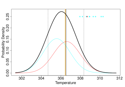
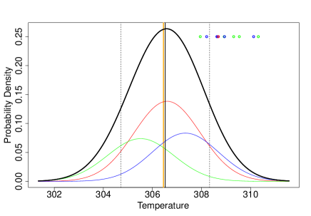
(a) (b)

 

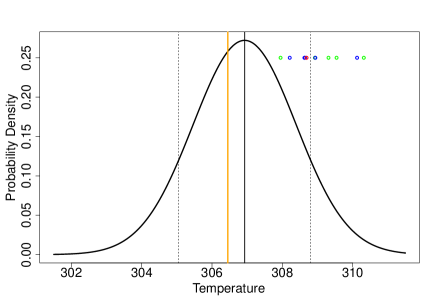
(c) (d)

Figure 2: (a) and (b): BMA; (c) and (d): EMOS density forecasts for 2m temperature for Debrecen valid on 02.07.2012. BMA PDFs with linear bias correction in two- and three-group cases (overall: thick black line; control: red line; sum of exchangeable members on (a): light blue line; on (b): green (odd members) and blue (even members) lines), EMOS predictive PDFs in two- and three-group cases (thick black line), ensemble members (circles with the same colours as the corresponding BMA PDFs), BMA/EMOS median forecasts (vertical black line), verifying observations (vertical orange line) and the first and last deciles (vertical dashed lines).

As typical example for illustrating the two different post-processing methods and groupings we consider temperature data and forecasts for Debrecen valid on 02.07.2012. Figures 2a and 2b show the BMA predictive PDFs in the two- and in the three-group case, the component PDFs corresponding to different groups, the median forecasts, the verifying observations, the first and last deciles and the ensemble members. Besides the EMOS predictive PDFs the same quantities can be seen in Figures 2c and 2d, too. On the considered date the spread of the ensemble is reasonable (the ensemble range equals 2.368 K) but all ensemble members overestimate the validating observation (306.45 K). Obviously the same holds for the ensemble median (308.927 K), while BMA median forecasts corresponding to the two- and three-group models (both equal to 306.524 K) are quite close to the true temperature. The point forecasts produced by the EMOS model are slightly worse (306.921 K for both groupings) but still outperform the ensemble median.

Figure 3: Mean CRPS of predictive distributions, MAE of BMA/EMOS median and RMSE of BMA/EMOS mean forecasts for temperature corresponding to two-group models for various training period lengths (BMA: solid and $\circ$; EMOS: dashed and $\Box$).

We start our data analysis by determining the optimal lengths of the training periods to be used for estimating the parameters of BMA and EMOS predictive distributions for 2m temperature and 10m wind speed. After finding them we compare the performances of BMA and EMOS post-processed forecasts using these optimal training period lengths. We remark that for EMOS models the parameter estimates are obtained by minimizing the CRPS values of the predictive PDFs.

4.1 Training period

Similarly to our previous studies (Baran et al., 2013a, ; Baran et al., 2013b, ) we proceed in the same way as Raftery et al., (2005) and determine the length of training period to be used for BMA and EMOS calibrations by comparing the MAE values of median forecasts, the RMSE values of mean forecasts, the CRPS values of predictive distributions and the coverages and average widths of $83.33\,\%$ central prediction intervals calculated from the predictive PDFs using training periods of length $10,11,\ldots,60$ calendar days. In order to ensure the comparability of the verification scores corresponding to different training period lengths we issue calibrated forecasts of temperature and wind speed for the period 01.06.2012 – 31.03.2013 (6 days with missing data are excluded). This means 298 calendar days following the first training period of maximal length of 60 days.

Temperature

For temperature data we consider BMA predictive PDF (3.3) with linear bias correction and EMOS model (3.7) with parameters minimizing the CRPS of probabilistic forecasts corresponding to the training data. We remark that in order to ensure a more direct comparison of the two models we also investigated the performance of the BMA predictive PDF (3.3) with parameter estimates minimizing the same verification score. It yielded sharper central prediction intervals and lower coverage for all training period length considered, but there were no significant differences in CRPS, MAE and RMSE values corresponding to different parameter estimation methods.

		Mean CRPS			MAE			RMSE
		opt.	opt.	day 35	opt.	opt.	day 35	opt.	opt.	day 35
		day	value	value	day	value	value	day	value	value
Two	BMA	$35$	$1.0900$	$1.0900$	$35$	$1.5230$	$1.5230$	$35$	$1.9914$	$1.9914$
groups	EMOS	$58$	$1.0734$	$1.0751$	$38$	$1.4862$	$1.4874$	$35$	$1.9504$	$1.9504$
Three	BMA	$35$	$1.0896$	$1.0896$	$35$	$1.5227$	$1.5227$	$36$	$1.9897$	$1.9899$
groups	EMOS	$36$	$1.0747$	$1.0756$	$28$	$1.4821$	$1.4901$	$28$	$1.9506$	$1.9576$

Table 2: Optimal training period lengths for temperature with respect to mean CRPS, MAE and RMSE, the corresponding optimal scores and scores at the chosen 35 days length.

Consider first the two-group situation. In Figure 3 the CRPS values of BMA and EMOS predictive distributions, MAE values of median and RMSE values of mean forecasts are plotted against the length of the training period. We remark that for normal EMOS model mean and median forecasts are obviously coincide. First of all it is noticeable that the results are very consistent for all diagnostics, i.e. the curves are similar for all measures. EMOS produces better verification scores and after 32 days there is no big difference among scores obtained with different training period lengths. In case of the BMA model CRPS, MAE and RMSE reach their minima at day 35 and this training period length gives the minimum of RMSE of the EMOS model, too (see Table 2). Although the minima of CRPS and MAE of the EMOS model are reached at days 58 and 38, respectively, the values at day 35 are very near to these minima as well.

Figure 4: Average width and coverage of $83.33\,\%$ BMA/EMOS central prediction intervals for temperature corresponding to two-group models for various training period lengths (BMA: solid and $\circ$; EMOS: dashed and $\Box$).

Figure 4 shows the average width and the coverage of the $83.33\,\%$ central prediction interval for both models considered. Similarly to the previous diagnostics, after 32 days all curves are rather flat showing only a slightly increasing trend. EMOS model yields significantly wider central prediction intervals for all training period lengths considered and its coverage is above the nominal value of $83.33\,\%$ (dashed line) for training periods longer than 12 days. Unfortunately, the coverage of the BMA model fails to reach the nominal value, but it is very close to $83.33\,\%$ from day 35 onwards. The maximal coverage is attained at day 37. Comparing the average width and coverage one can observe that they have opposite behaviour, i.e. the average width values favour shorter training periods, while the coverage figures prefer longer ones. On the other hand, the trend of the average width values is rather flat after day 30 (or so). For any case a reasonable compromise ought to be found, which is at the range of 30 - 40 days.

As a summary it can be said that a 35 days training period seems to be an acceptable choice both for the BMA and for the EMOS models (particularly see conclusions based on Figure 3, which are not compromised by the other two diagnostics at Figure 4).

Figure 5: Mean CRPS of predictive distributions, MAE of BMA/EMOS median and RMSE of BMA/EMOS mean forecasts for wind speed corresponding to two-group models for various training period lengths (Gamma BMA: solid and $\circ$; truncated normal BMA: dotted and $\diamond$; EMOS: dashed and $\Box$).

Very similar conclusions can be drawn for the three-group models. The overall behaviours of the two post-processing methods for the various diagnostics (not shown) is very similar to those of their two-group counterparts. EMOS model provides lower CRPS, MAE and RMSE values and higher coverage combined with wider central prediction interval all over the time periods. In terms of specific values the minima of CRPS and MAE for the BMA model are reached again at day 35, while the RMSE takes its minimum at day 36 (the value at day 35 is very near to this minimum, see Table 2). For the EMOS model CRPS, MAE and RMSE reach their minima in the range of 28 - 36 days and values at day 35 are again very close to these minima.

Figure 6: Average width and coverage of $83.33\,\%$ BMA/EMOS central prediction intervals for wind speed corresponding to two-group models for various training period lengths (Gamma BMA: solid and $\circ$; truncated normal BMA: dotted and $\diamond$; EMOS: dashed and $\Box$).

Regarding the average width, shorter training periods yields sharper central prediction intervals. The coverage for the EMOS model is above the nominal value for training periods longer than 14 days, while the maximal coverage of the BMA model is reached at day 59. However, as in general shorter training periods are preferred, a reasonable compromise is to consider the 35 - 38 days interval where the BMA coverage is also very high. Hence, the training period proposed for the two-group model can be kept for the three-group model as well, therefore for temperature we suggest the use of a training period of length 35 days for all the investigated post-processing methods.

Wind speed

To calibrate ensemble forecasts of wind speed we apply gamma BMA model (3.4), truncated normal BMA model (3.5) and EMOS model (3.8). In the latter case, similarly to EMOS calibration of temperature forecasts, estimation of parameters is done by minimizing the CRPS of probabilistic forecasts corresponding to the training data.

First, consider again the case when we have two groups of exchangeable ensemble members. Generally the various scores have rather flat evolution with respect to the training lengths (see Figures 5 and 6). It is particularly true after day 25, which would suggest that basically any training length longer than 25 days might be an acceptable choice. Observe that the order of different methods with respect to a given score remains the same for all training period lengths. Truncated normal BMA produces the lowest CRPS values, while the best MAE and RMSE values correspond to EMOS post-processing. For any case if we wanted to pick up a single training period length as an optimal one, 43 days would be a reasonable choice. This is the value where the minima of CRPS of all three methods, the minima of RMSE of gamma BMA and of EMOS and the minimum of MAE of EMOS are reached (see Table 3). The other two scores corresponding to EMOS model attain their minima at day 59, however values corresponding to day 43 are practically the same. Finally, the minimum of MAE of the gamma BMA model is reached at day 47, while the value at day 43 is the second smallest one.

EMOS post-processing yields the widest central prediction intervals and the highest coverage (Figure 6) which is above the nominal level for all considered training period lengths. The $83.33\,\%$ central prediction intervals corresponding to the truncated normal BMA model are significantly sharper than those of the EMOS combined with a coverage varying between $83.89\,\%$ and $86.14\,\%$. Gamma BMA results in even narrower central prediction intervals but its coverage never reaches the nominal level. The maximal coverage is attained at days 38 and 49. In this way a 43 days training period length is also acceptable from the point of view of central prediction intervals.

		Mean CRPS			MAE			RMSE
		opt.	opt.	day 43	opt.	opt.	day 43	opt.	opt.	day 43
		day	value	value	day	value	value	day	value	value
Two	BMA, g.	$43$	$0.7551$	$0.7551$	$47$	$1.0692$	$1.0694$	$43$	$1.4145$	$1.4145$
groups	BMA, tr.	$43$	$0.6933$	$0.6933$	$59$	$1.0385$	$1.0389$	$59$	$1.3657$	$1.3658$
	EMOS	$43$	$0.7375$	$0.7375$	$43$	$1.0335$	$1.0335$	$43$	$1.3521$	$1.3521$
Three	BMA, g.	$43$	$0.7559$	$0.7559$	$42$	$1.0690$	$1.0691$	$42$	$1.3940$	$1.3941$
groups	BMA, tr.	$39$	$0.6930$	$0.6930$	$39$	$1.0377$	$1.0382$	$39$	$1.3545$	$1.3551$
	EMOS	$43$	$0.7393$	$0.7393$	$43$	$1.0342$	$1.0342$	$43$	$1.3540$	$1.3540$

Table 3: Optimal training period lengths for wind speed with respect to mean CRPS, MAE and RMSE, the corresponding optimal scores and scores at the chosen 43 days length.

The analysis of verification scores corresponding to the alternative grouping of ensemble members (not shown) leads again to very similar results. The most important difference between the two-group and three-group models is that forming three groups (especially for training periods longer than 20 days) improves MAE and RMSE values of the truncated normal BMA model and they become very close to the corresponding values of EMOS. For the three-group EMOS model all three verification scores reach their minima at day 43 and this is the training period length where the minimal CRPS and the second smallest values of MAE and RMSE of the gamma BMA model are attained (see Table 3). For the latter model the global minima of MAE and RMSE are at day 42. In case of truncated normal BMA post-processing CRPS, MAE and RMSE have their minima at day 39, but since these curves are rather flat, values corresponding to a training period of length 43 days are very near. In this way a 43 days training period seems to be acceptable for both groupings of ensemble members.

4.2 Ensemble calibration using BMA and EMOS post-processing

According to the results of the previous section to compare the performance of BMA and EMOS post-processing on the 11 member ALADIN-HUNEPS ensemble we use rolling training periods of lengths 35 days for temperature and 43 days for wind speed.

Temperature

For post-processing ensemble forecasts of temperature we consider the BMA model (3.3) with all three bias correction methods introduced in Section 3.1 (linear, additive, none) and EMOS model minimizing the CRPS of probabilistic forecasts corresponding to the training data. The application of three different BMA bias correction methods is justified by a previous study dealing with statistical calibration of the ALADIN-HUNEPS temperature forecasts (Baran et al., 2013b, ), where the simplest BMA model without bias correction showed the best overall performance (although that study was using different ALADIN-HUNEPS dataset period, which preceded the one investigated in this article).

The use of a 35 day rolling training period implies that ensemble members, validating observations and predictive PDFs are available for the period 07.05.2012 – 31.03.2013 (having 323 calendar days just after the first 35 days training period). This time interval starts nearly 4 weeks earlier than the one used for determination of the optimal training period length.

Figure 7: PIT histograms for BMA and EMOS post-processed forecasts of temperature using two- and three-group models.

The first step in checking the calibration of our post-processed forecasts is to have a look at their probability integral transform (PIT) histograms. The PIT is the value of the predictive cumulative distribution evaluated at the verifying observations (Raftery et al.,, 2005), which provides a good and easily interpretable measure about the possible improvements of the under-dispersive character of the raw ensemble. The closer the histogram to the uniform distribution, the better the calibration is. In Figure 7 PIT histograms corresponding to all three versions of the BMA model and to the EMOS model are displayed both in the two- and in the three-group case. A comparison to the verification rank histogram of the raw ensemble (see Figure 1) shows that at every case post-processing significantly improves the statistical calibration of the forecasts. However, the BMA model without bias correction and the EMOS model now become slightly over-dispersive, while at the same time for the BMA models with linear and additive bias correction one can accept uniformity. This visual perception is confirmed by the $p$-values of Kolmogorov-Smirnov tests for uniformity of the PIT values (see Table 4). Therefore, the BMA model with additive bias correction produces the best PIT histograms (the linear bias correction case is just slightly worse), while the fit of the BMA model without bias correction and that of the EMOS model are rather poor. One can additionally observe that the three-group models systematically outperform the two-group ones.

	BMA model with bias correction			EMOS model
	linear	additive	none
Two groups	$0.1393$	$0.2405$	$2.2\times 10^{-10}$	$9.4\times 10^{-7}$
Three groups	$0.2281$	$0.4617$	$4.1\times 10^{-9}$	$8.6\times 10^{-5}$

Table 4: $p$-values of Kolmogorov-Smirnov tests for uniformity of PIT values corresponding to predictive distributions of temperature.

		Mean	MAE		RMSE		Average	Coverage
		CRPS	median	mean	median	mean	width	($\%$)
	BMA, lin.	$1.0815$	$1.5101$	$1.5097$	$1.9789$	$1.9765$	$5.1375$	$83.00$
Two	BMA, add.	$1.1029$	$1.5395$	$1.5329$	$2.0028$	$1.9871$	$5.5146$	$84.21$
groups	BMA, none	$1.1131$	$1.5536$	$1.5444$	$2.0167$	$2.0014$	$5.7191$	$84.80$
	EMOS	$1.0693$	$1.4768$	$1.4768$	$1.9387$	$1.9387$	$5.7735$	$87.55$
	BMA, lin.	$1.0801$	$1.5082$	$1.5059$	$1.9767$	$1.9726$	$5.1369$	$83.28$
Three	BMA, add.	$1.0998$	$1.5346$	$1.5254$	$1.9962$	$1.9783$	$5.5096$	$84.12$
groups	BMA, none	$1.1123$	$1.5509$	$1.5407$	$2.0156$	$1.9988$	$5.7095$	$85.11$
	EMOS	$1.0670$	$1.4743$	$1.4743$	$1.9399$	$1.9399$	$5.6143$	$86.07$
Raw ensemble		$1.2284$	$1.5674$	$1.5512$	$2.0434$	$2.0131$	$3.9822$	$60.53$

Table 5: Mean CRPS of probabilistic, MAE and RMSE of median/mean forecasts, average width and coverage of $83.33\,\%$ central prediction intervals for temperature.

In Table 5 verification measures of probabilistic and point forecasts calculated using BMA and EMOS models are given together with the corresponding scores of the raw ensemble. By examining these results, one can clearly observe again the obvious advantage of post-processing with respect to the raw ensemble. This is quantified in decrease of CRPS, MAE and RMSE values and in a significant increase in the coverage of the $83.33\,\%$ central prediction intervals. On the other hand, the post-processed forecasts are less sharp (e.g. $83.33\,\%$ central prediction intervals are around $30\,\%-40\,\%$ wider than the raw ensemble range). This fact is coming from the small dispersion of the raw ensemble, as also seen in the verification rank histogram of Figure 1. Furthermore, BMA and EMOS models distinguishing three exchangeable groups of ensemble members slightly outperform their two-group counterparts (in agreement with the interpretations based on the PIT histograms). Comparing the different post-processing methods it is noticeable that on the one hand EMOS produces the lowest CRPS, MAE and RMSE values both in the two- and in the three-group case although with coverages highly above the targeted $83.33\,\%$. On the other hand, in terms of CRPS, MAE and RMSE the behaviour of the BMA model with linear bias correction is just slightly worse and at the same time this method produces the sharpest predictive PDFs and the best approximation of the nominal coverage. Taking also into account the fit of the PIT values to the uniform distribution (see Figure 7 and Table 4 again) one can conclude that overall from the four competing post-processing methods the BMA model with linear bias correction shows the best performance. These results are not in contradiction with the ones for a previous period (see Baran et al., 2013b , where the no bias correction case proved to be the optimal) since the characteristics of the raw ALADIN-HUNEPS system had been slightly changed in between. The coverage of the system had been significantly improved (from $46\,\%$ to $60\,\%$) although the latest system became slightly biased (as compared to the previously examined one). Therefore, due to the existence of the bias it is not surprising that one of the versions with bias correction has the best behaviour.

Wind speed

Figure 8: PIT histograms for BMA and EMOS post-processed forecasts of wind speed using two- and three-group models.

According to results of Section 4.1, to compare the performance of gamma BMA (3.4), truncated normal BMA (3.5) and EMOS (3.8) post-processing on the 11 member ALADIN-HUNEPS ensemble we use a training period of length 43 calendar days. In this way ensemble members, validating observations and predictive distributions are available for the period 15.05.2012 – 31.03.2013 (313 calendar days).

	BMA model		EMOS model
	gamma	tr. normal
Two groups	$0.1812$	$0.0023$	$1.8\times 10^{-5}$
Three groups	$0.2085$	$0.0043$	$9.6\times 10^{-7}$

Table 6: $p$-values of Kolmogorov-Smirnov tests for uniformity of PIT values corresponding to predictive distributions of wind speed.

First, consider again the PIT histograms of various calibration methods, which are displayed in Figure 8. Compared to the verification rank histogram of the wind speed ensemble (see Figure 1) the statistical post-processing induced improvements are obvious, however, e.g. in case of EMOS both corresponding PIT histograms are highly over-dispersive. In that sense the temperature calibration (as shown in the previous chapter) is more successful than the wind speed one. The $p$-values of Kolmogorov-Smirnov tests given in Table 6 also show that EMOS models produce the poorest fit, while for gamma BMA models one can accept uniformity. In case of BMA calibration the three-group models again outperform the two-group ones, while for EMOS the situation is the reverse. A similar behaviour can be observed in Table 7, where the verification scores of probabilistic and point forecasts calculated using BMA and EMOS post-processing and the corresponding measures of the raw ensemble are given. Considering first the probabilistic forecasts (in terms of CRPS, average width of central prediction interval and coverage) one can observe that the calibrated forecasts are smaller in CRPS, wider in central prediction intervals and higher in coverage compared to the raw ensemble. Equally, to the two- and in three-group cases the smallest CRPS values belong to the truncated normal BMA model, while gamma BMA post-processing produces the best approximation of the nominal coverage of $83.33\,\%$. Regarding the point forecasts (median and mean) calculated from the truncated normal BMA and EMOS predictive PDFs, generally there are smaller MAE and RMSE values than those of the raw ensemble. However, there is an exception for the gamma BMA model since these scores are higher indicating degradations. A possible explanation might be related to the fact that in the investigated period (15.05.2012 – 31.03.2013) both the raw ensemble median and the ensemble mean slightly overestimate the validating observations (their average biases (standard errors) are $0.0907\ (0.0249)$ and $0.0972\ (0.0244)$, respectively). Therefore, the small bias should be removed by relevant bias corrections. On the other hand, we believe that the simplest bias correction procedure of the gamma BMA model cannot eliminate these inaccuracies, moreover, it might introduce some additional errors. It is a matter of fact that in the two-group case the average biases of the median and mean of the gamma BMA predictive PDF are $-0.1935$ and $-0.1318$ with standard errors of $0.0250$ and $0.0253$, respectively, while for the EMOS model showing the lowest MAE and RMSE values these biases are only $-0.0340$ and $0.0312$, both having a standard error of $0.0249$. Therefore, the EMOS model is able to compensate for the existing biases, which is also the case for the truncated normal BMA case, but not for the gamma BMA calibration. The difference in behaviour between the two BMA calibration methods is attributed to the more sophisticated bias correction algorithm, which is applied for the truncated normal BMA case.

		Mean	MAE		RMSE		Average	Coverage
		CRPS	median	mean	median	mean	width	($\%$)
Two	BMA, g.	$0.7601$	$1.0747$	$1.0895$	$1.4176$	$1.4267$	$3.7151$	$81.87$
groups	BMA, tr. n.	$0.6982$	$1.0446$	$1.0478$	$1.3693$	$1.3772$	$3.7621$	$85.46$
	EMOS	$0.7409$	$1.0384$	$1.0451$	$1.3583$	$1.3602$	$3.9777$	$88.06$
Three	BMA, g.	$0.7612$	$1.0754$	$1.0828$	$1.4192$	$1.4052$	$3.7064$	$82.03$
groups	BMA, tr. n.	$0.6980$	$1.0437$	$1.0449$	$1.3696$	$1.3649$	$3.7498$	$85.08$
	EMOS	$0.7431$	$1.0396$	$1.0469$	$1.3597$	$1.3633$	$4.0294$	$88.25$
Raw ensemble		$0.8029$	$1.0688$	$1.0549$	$1.3980$	$1.3728$	$2.8842$	$68.22$

Table 7: Mean CRPS of probabilistic, MAE and RMSE of median/mean forecasts, average width and coverage of $83.33\,\%$ central prediction intervals for wind speed.

To summarize, gamma BMA model outperforms the other two methods in terms of fit of PIT values and in sharpness and coverage of central prediction intervals, but it has the highest CRPS and very poor verification scores for the point forecasts. MAE and RMSE values corresponding to EMOS and truncated normal BMA are lower than those of the raw ensemble and rather similar to each other. From these two methods truncated normal BMA produces much lower CRPS, sharper central prediction intervals and better fit of PIT values to the uniform distribution, so we conclude that the overall performance of this method is the best for the calibration of the wind speed raw ensemble forecasts.

5 Discussion and conclusions

In this paper we have compared different versions of the BMA and EMOS statistical post-processing methods in order to improve the calibration of 2m temperature and 10m wind speed forecasts of the ALADIN-HUNEPS system. First, we have demonstrated the weaknesses of the ALADIN-HUNEPS raw ensemble system being under-dispersive and therefore uncalibrated. We have indicated that the under-dispersive character of the ALADIN-HUNEPS system had been improved compared to studies based on a former dataset, however more enhancements are still needed. On the other hand, the latest dataset shows some features of bias of ALADIN-HUNEPS, which were inexistent in earlier studies. This fact has an influence on the optimal choice of statistical calibration, since the use of bias correction is getting more essential. Some standard measures were applied, which are related to the characteristics of the ensemble probability density functions and also the point forecasts as described by the mean/median of the ensemble. The various systems improve different aspects of the ensemble, however overall both the BMA and the EMOS method is capable to deliver significant improvements on the raw ALADIN-HUNEPS ensemble forecasts (for temperature and wind speed as well). Generally the best BMA method slightly outperforms the EMOS technique (although it should not be forgotten that for instance in terms of point forecasts EMOS is better than BMA).

Acknowledgments.    Research was supported by the Hungarian Scientific Research Fund under Grant No. OTKA NK101680 and by the TÁMOP-4.2.2.C-11/1/KONV-2012-0001 project. The project has been supported by the European Union, co-financed by the European Social Fund. Essential part of this work was made during the visiting professorship of the first author at the Institute of Applied Mathematics of the University of Heidelberg. The authors are indebted to Tilmann Gneiting for his useful suggestions and remarks, to Thordis Thorarinsdottir for the R codes of EMOS for wind speed and to Mihály Szűcs from the HMS for providing the data.

References

- Baran, (2013) Baran, S. (2013) Probabilistic wind speed forecasting using Bayesian model averaging with truncated normal components. Comput. Stat. Data. Anal., under review (arXiv:1305:1184).
- (2) Baran, S., Horányi, A. and Nemoda, D. (2013a) Statistical post-processing of probabilistic wind speed forecasting in Hungary. Meteorol. Z. 22, 273–282.
- (3) Baran, S., Horányi, A. and Nemoda, D. (2013b) Probabilistic temperature forecasting with statistical calibration in Hungary. Meteorol. Atmos. Phys., under review (arXiv:1303.2133).
- Buizza et al., (1993) Buizza, R., Tribbia, J., Molteni, F. and Palmer, T. (1993) Computation of optimal unstable structures for a numerical weather prediction system. Tellus A 45, 388–407.
- Descamps et al., (2009) Descamps, L., Labadie, C., Joly, A. and Nicolau, J. (2009) Ensemble Prediction at Météo France (poster introduction by Olivier Riviere) 31st EWGLAM and 16th SRNWP meetings, September 28 – October 1, 2009. Available at: http://srnwp.met.hu/Annual_Meetings/2009/download/sept29/morning/posterpearp.pdf
- Eckel and Mass, (2005) Eckel, F. A. and Mass, C. F. (2005) Effective mesoscale, short-range ensemble forecasting. Wea. Forecasting 20, 328–350.
- Fraley et al., (2010) Fraley, C., Raftery, A. E. and Gneiting, T. (2010) Calibrating multimodel forecast ensembles with exchangeable and missing members using Bayesian model averaging. Mon. Wea. Rev. 138, 190–202.
- Fraley et al., (2009) Fraley, C., Raftery, A. E., Gneiting, T. and Sloughter, J. M. (2009) EnsembleBMA: An R package for probabilistic forecasting using ensembles and Bayesian model averaging. Technical Report 516R, Department of Statistics, University of Washington. Available at: www.stat.washington.edu/research/reports/2008/tr516.pdf
- Fraley et al., (2011) Fraley, C., Raftery, A. E., Gneiting, T., Sloughter, J. M. and Berrocal, V. J. (2011) Probabilistic weather forecasting in R. The R Journal 3, 55–63.
- Gebhardt et al., (2011) Gebhardt, C., Theis, S. E., Paulat, M. and Bouallègue, Z. B. (2011) Uncertainties in COSMO-DE precipitation forecasts introduced by model perturbations and variation of lateral boundaries. Atmos. Res. 100, 168–177.
- Gneiting, (2011) Gneiting, T. (2011) Making and evaluating point forecasts. J. Amer. Statist. Assoc. 106, 746–762.
- Gneiting and Raftery, (2007) Gneiting, T. and Raftery, A. E. (2007) Strictly proper scoring rules, prediction and estimation. J. Amer. Statist. Assoc. 102, 359–378.
- Gneiting et al., (2005) Gneiting, T., Raftery, A. E., Westveld, A. H. and Goldman, T. (2005) Calibrated probabilistic forecasting using ensemble model output statistics and minimum CRPS estimation. Mon. Wea. Rev. 133, 1098–1118.
- Hágel, (2010) Hágel, E. (2010) The quasi-operational LAMEPS system of the Hungarian Meteorological Service. Időjárás 114, 121–133.
- Horányi et al., (2006) Horányi, A, Kertész, S., Kullmann, L. and Radnóti, G. (2006) The ARPEGE/ALADIN mesoscale numerical modeling system and its application at the Hungarian Meteorological Service. Időjárás 110, 203–227.
- Horányi et al., (2011) Horányi, A., Mile, M. and Szűcs, M. (2011) Latest developments around the ALADIN operational short-range ensemble prediction system in Hungary. Tellus A 63, 642–651.
- Justus et al., (1978) Justus, C. G., Hargraves, W. R., Mikhail, A. and Graber, D. (1978) Methods for estimating wind speed frequency distributions. J. Appl. Meteor. 17, 350–353.
- Labadie et al., (2012) Labadie, C., Descamps,L., Cebron, P. and Michel, Y. (2012) PEARP initialization with Ensemble Data Asssimilation and Singular Vectors. International Conference on Ensemble Methods in Geophysical Sciences, Toulouse, France, November 12–16, 2012. Available at: http://www.meteo.fr/cic/meetings/2012/ensemble.conference/presentations/session07/2.pdf
- Leutbecher and Palmer, (2008) Leutbecher, M. and Palmer, T. N. (2012) Ensemble forecasting. J. Comp. Phys. 227, 3515–3539.
- Pinson and Hagedorn, (2012) Pinson, P. and Hagedorn, R. (2012) Verification of the ECMWF ensemble forecasts of wind speed against analyses and observations. Meteorol. Appl. 19, 484–500.
- Raftery et al., (2005) Raftery, A. E., Gneiting, T., Balabdaoui, F. and Polakowski, M. (2005) Using Bayesian model averaging to calibrate forecast ensembles. Mon. Wea. Rev. 133, 1155–1174.
- Sloughter et al., (2010) Sloughter, J. M., Gneiting, T. and Raftery, A. E. (2010) Probabilistic wind speed forecasting using ensembles and Bayesian model averaging. J. Amer. Stat. Assoc. 105, 25–37.
- Sloughter et al., (2007) Sloughter, J. M., Raftery, A. E., Gneiting, T. and Fraley, C. (2007) Probabilistic quantitative precipitation forecasting using Bayesian model averaging. Mon. Wea. Rev. 135, 3209–3220.
- Thorarinsdottir and Gneiting, (2010) Thorarinsdottir, T. L. and Gneiting, T. (2010) Probabilistic forecasts of wind speed: ensemble model output statistics by using heteroscedastic censored regression. J. Roy. Statist. Soc. Ser. A 173, 371–388.
- Toth and Kalnay, (1997) Toth, Z. and Kalnay, E. (1997) Ensemble forecasting at NCEP and the breeding method. Mon. Wea. Rev. 125, 3297–3319.
- Wilks, (2011) Wilks, D. S. (2011) Statistical Methods in the Atmospheric Sciences. 3rd ed., Elsevier, Amsterdam.
- Wilks and Hamil, (2007) Wilks, D. S. and Hamill, T. M. (2007) Comparison of ensemble-MOS methods using GFS reforecasts. Mon. Wea. Rev. 135, 2379–2390.