Plane correlations and hydrodynamic simulations of heavy ion collisions

Abstract

We use a nonlinear response formalism to describe the event plane correlations measured by the ATLAS collaboration. With one exception ($\left\langle\cos(2\Psi_{2}-6\Psi_{3}+4\Psi_{4})\right\rangle$), the event plane correlations are qualitatively reproduced by considering the linear and quadratic response to the lowest cumulants. For the lowest harmonics such as $\left\langle\cos(2\Psi_{2}+3\Psi_{3}-5\Psi_{5})\right\rangle$, the correlations are quantitatively reproduced, even when the naive Glauber model prediction has the wrong sign relative to experiment. The quantitative agreement for the higher plane correlations (especially those involving $\Psi_{6}$) is not as good. The centrality dependence of the correlations is naturally explained as an average of the linear and quadratic response.

I Introduction

The collective expansion of the deconfined fireball created in high energy heavy-ion collisions maps the initial state of the Quark-Gluon Plasma (QGP) to the final state particle spectrum. The measured correlations in this spectrum can clarify the initial conditions and subsequent expansion dynamics of the QGP Heinz and Snellings (2013); Hippolyte and Rischke (2013); Teaney (2009).

On an event-event basis the azimuthal distribution of produced particles can be decomposed into a Fourier series

$$\frac{dN}{d\phi_{\bm{p}}}=\frac{N}{2\pi}\,\left(1+2\sum_{n=1}^{\infty}v_{n}\cos(n\phi_{\bm{p}}-n\Psi_{n})\right)\,,$$ (1)

and the measured two particle correlation function determines the root mean square of the these harmonics, $\sqrt{\left\langle v_{n}^{2}\right\rangle}$. The magnitude of these harmonics is reasonably reproduced by event-by-event viscous hydrodynamics provided the shear viscosity is not too large Heinz and Snellings (2013). The correlations between the harmonics can provide new tests of the hydrodynamic description, constrain the simulation parameters, and provide an estimate of the uncertainties in the computation. In this work we will describe the correlations between the observed event plane angles $\Psi_{n}$ in order to clarify the expansion dynamics, and ultimately to determine the shear viscosity of the QGP with credible systematic error bars.

Clearly, an important input to the hydrodynamic simulations is the distribution of energy density in the transverse plane, which is usually estimated from the known probability distribution of nucleons in the incoming nuclei. There is reasonable evidence, both experimental Alver and Roland (2010) and theoretical Qiu and Heinz (2011), that $v_{2}$ and $v_{3}$ are to a good approximation linearly proportional to the corresponding angular fluctuations in the transverse energy density. However, event-by-event hydrodynamic simulations have shown that the higher harmonics, $v_{4}$ and $v_{5}$, reflect both the response to corresponding angular harmonics in the initial state, and the non-linear hydrodynamic response which mixes lower order harmonics Qiu and Heinz (2011); Gardim et al. (2012). For example, the $5$-th flow harmonic, $v_{5}$, is determined in part by the medium response to the $5$-th harmonic of the initial energy density distribution, and in part by the non-linear mixing between $v_{2}$ and $v_{3}$. Such mode-mixing is especially important at high $p_{T}$ where the non-linearities of the phase-space distribution play an important role Borghini and Ollitrault (2006). Indeed, there are indications that the dominant source of mode mixing comes from freezeout as opposed to the hydrodynamic evolution Floerchinger et al. (2013). Motivated by these simulation results, and especially the simulation analysis of Ref. Gardim et al. (2012), we developed a non-linear response formalism to describe the mixing between modes of different order, and we investigated how the response coefficients depend on centrality, shear viscosity, and transverse momentum Teaney and Yan (2012).

These theoretical calculations preceded the corresponding experimental studies by the ATLAS Collaboration (May, 2012) and ALICE collaborations Bilandzic (2013), which qualitatively confirmed the mode mixing picture by measuring significant correlations between the event-plane angles of different orders, e.g. between $\Psi_{2}$,$\Psi_{3}$, and $\Psi_{5}$. Event-by-event hydrodynamics Qiu and Heinz (2012) and AMPT calculations Bhalerao et al. (2013) largely reproduce the structure of these correlations. The goal of this paper is to compare the response formalism outlined in our previous work to the event-plane correlations measured by the ATLAS collaboration Teaney and Yan (2012).

As discussed more technically in Section II.2 we will use a non-linear response formalism to describe the observed event plane correlations, rather than event-by-event hydrodynamics. In practice, this means that we decompose the initial state into an average event plus small fluctuations, which are systematically analyzed with cumulants. The linear and quadratic response to each cumulant is found by perturbing the average background, and finally the observed plane correlations are found by weighting the response functions with the spectrum of fluctuations. Thus, the response formulation provide a transparent link between the initial state and the final state, which contains only the linear and quadratic response through a specified order in the cumulant expansion. As we will see, this approach reproduces a lot of the observed event plane correlations, suggesting that most of the microscopic details of the initial state (beyond the lowest cumulants) are irrelevant. Ideally, a limited number of initial state parameters can be extracted from experiment, and compared to available theoretical frameworks such as the Color Glass Condensate to demonstrate the consistency and uniqueness of the approach. There are indications that the spectrum of fluctuations from the Color Glass Condensate is consistent with the observed harmonics Gale et al. (2013), but the uniqueness of this approach is not obvious.

A review of the non-linear flow response formalism will be given in Section II. This has several ingredients. First, the spectrum of initial fluctuations in various Glauber type models is described in Section II.1, and this spectrum is analyzed with the cumulant and moment expansions. Then, we describe how the response coefficients are calculated, and how these coefficients determine the plane correlations in Section II.2 and Section II.3. Finally, we compare the response formalism to the ATLAS data in Section III and discuss the results.

Throughout the paper $\Phi_{n}$ will denote participant plane angle based on the cumulants rather than moments. (The correlations in the Glauber model between the cumulant angles $\Phi_{n}$ are markedly different from the correlations found using the analogous moment based angles – see Section II.1.) $\Psi_{n}$ denotes the event plane angle extracted from the final state momentum spectra.

II Review of nonlinear flow response formalism

II.1 Characterizing the initial state with cumulants

As discussed in the introduction, an important input to the hydrodynamic calculations is the spectrum of initial fluctuations. This spectrum is traditionally Alver and Roland (2010) quantified with the participant plane anisotropy based on moments

$$\varepsilon_{n}e^{in\Phi_{n}}\equiv-\frac{\left\langle r^{n}e^{in\phi_{r}}\right\rangle}{\left\langle r^{n}\right\rangle}\qquad\qquad\qquad{\mbox{(Not used).}}$$ (2)

Here the brackets $\left\langle\ldots\right\rangle$ denote an average over the participating nucleons of a single event, while $re^{i\phi_{r}}=x+i\,y$ notates the transverse coordinates of the participants. It is convenient to use a complex notation $z\equiv x+iy$ so that ${\varepsilon}_{n}e^{in\Phi_{n}}=-\left\langle z^{n}\right\rangle/\left\langle r^{n}\right\rangle$. As emphasized in our previous work, it is often useful to characterize the fluctuations with cumulants rather than moments. The cumulants subtract off the lower order correlation functions of $z$ to describe the irreducible correlations

$${\varepsilon}_{n}e^{in\Phi_{n}}\equiv-\frac{1}{r^{n}}\left[\left\langle z^{n}\right\rangle-{\rm subtractions}\right]\,.$$ (3)

For example, the fourth order cumulant is

$${\varepsilon}_{4}e^{i4\Phi_{4}}\equiv-\frac{1}{\left\langle r^{4}\right\rangle}\left[\left\langle z^{4}\right\rangle-3\left\langle z^{2}\right\rangle^{2}\right]\,,$$ (4)

where the factor of three arises because there are three ways to pair four objects. Here and below we have assumed that we are working in the center of mass coordinate system where $\left\langle z\right\rangle=0$. The usefulness of cumulants can be understood by considering a Gaussian distribution,

$$\rho(x,y)\propto e^{-\frac{x^{2}}{2\left\langle x^{2}\right\rangle}-\frac{y^{2}}{2\left\langle y^{2}\right\rangle}}\,,$$ (5)

whose fourth order moment anisotropy $\left\langle z^{4}\right\rangle$ is non-zero, and is trivially correlated with the eccentricity, $\left\langle z^{2}\right\rangle$. The fourth order cumulant takes out these trivial correlations, and for a Gaussian distribution we have ${\varepsilon}_{4}\propto\left\langle z^{4}\right\rangle-3\left\langle z^{2}\right\rangle=0$.

The azimuthal anisotropies through ${\varepsilon}_{6}$ are

$${\mathcal{E}}_{2}\equiv{\varepsilon}_{2}e^{i2\Phi_{2}}\equiv -\frac{\left\langle z^{2}\right\rangle}{\left\langle r^{2}\right\rangle}\,,$$ (6)

$${\mathcal{E}}_{3}\equiv{\varepsilon}_{3}e^{i3\Phi_{3}}\equiv -\frac{\left\langle z^{3}\right\rangle}{\left\langle r^{3}\right\rangle}\,,$$ (7)

$${\mathcal{E}}_{4}\equiv{\varepsilon}_{4}e^{i4\Phi_{4}}\equiv -\frac{1}{\left\langle r^{4}\right\rangle}\left[\left\langle z^{4}\right\rangle-3\left\langle z^{2}\right\rangle^{2}\right]\,,$$ (8)

$${\mathcal{E}}_{5}\equiv{\varepsilon}_{5}e^{i5\Phi_{5}}\equiv -\frac{1}{\left\langle r^{5}\right\rangle}\left[\left\langle z^{5}\right\rangle-10\left\langle z^{2}\right\rangle\left\langle z^{3}\right\rangle\right]\,,$$ (9)

$${\mathcal{E}}_{6}\equiv{\varepsilon}_{6}e^{i6\Phi_{6}}= -\frac{1}{\left\langle r^{6}\right\rangle}\left[\left\langle z^{6}\right\rangle-15\left\langle z^{4}\right\rangle\left\langle z^{2}\right\rangle-10\left\langle z^{3}\right\rangle^{2}+30\left\langle z^{2}\right\rangle^{3}\right]\,,$$ (10)

where ${\mathcal{E}}_{n}={\varepsilon}_{n}e^{in\Phi_{n}}$ denotes the eccentricity and its phase. The ${\varepsilon}_{1}$ which drives $v_{1}$ is a special case, and is given by

$${\mathcal{E}}_{1}={\varepsilon}_{1}e^{i\Phi_{1}}\equiv-\frac{1}{\left\langle r^{3}\right\rangle}\left\langle z^{2}z^{*}\right\rangle\,.$$ (11)

Given an initial state Glauber model for the distribution of nucleons such as Glissando Broniowski et al. (2009) or the Phobos Monte Carlo Glauber model Alver et al. (2008) one can calculate the correlations between the angles $\Phi_{n}$. Fig. 1 and Fig. 2 show such a calculation from the Phobos Monte-Carlo model. Here and below the double brackets $\left\langle\!\left\langle\ldots\right\rangle\!\right\rangle$ indicate an average over events, while the single brackets $\langle\ldots\rangle$ denote an average over one event. In the Phobos Glauber the participant centers are used to define the averages in eq. (6), while in the Glissando model a slightly different prescription is used, which is based on the wounding profile of the nucleon Broniowski et al. (2009).

Figure 1: Participant 2-plane correlations from Phobos Monte Carlo Glauber model Alver et al. (2008) as measured by the cumulant and moment expansions. The measured event plane correlations Collaboration (May, 2012) are presented for reference and as a point of contact, and are not supposed to be directly compared to the Glauber model results.

Figure 2: Participant 3-plane correlations from Phobos Monte Carlo Glauber model Alver et al. (2008) as measured by the cumulant and moment expansions. The measured event plane correlations Collaboration (May, 2012) are presented for reference and as a point of contact, and are not supposed to be directly compared to the Glauber model results.

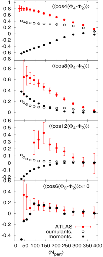
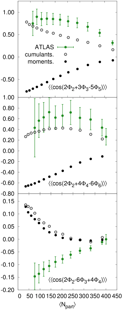
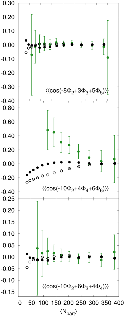
It is interesting to compare the correlations between the cumulant and moment based angles. For example, the $\left\langle\!\left\langle\cos 4(\Phi_{4}-\Phi_{2})\right\rangle\!\right\rangle$ correlation is strongly negative with the moment based definitions, while the corresponding correlations with cumulant angles are positive. In the moment definition the $\Phi_{4}$,$\Phi_{2}$ correlation arises because the fourth order eccentricity ${\mathcal{E}}_{4}$ is trivially correlated with the second order eccentricity ${\mathcal{E}}_{2}$ through the average geometry. These trivial geometric correlations are removed with the cumulant definition, and the residual correlation is positive. The correlation between $\Psi_{4}$ and $\Psi_{2}$ seen in the data is positive, but does not seem to be directly related to the participant plane correlation between $\Phi_{4}$ and $\Phi_{2}$. The interpretation of the data is described in Section III.

II.2 Formulation of flow response

The harmonic flow $v_{n}$ and the corresponding flow angle $\Psi_{n}$ are defined by the Fourier decomposition of the final state particle spectrum,

$$\frac{dN}{d\phi_{p}}=\frac{N}{2\pi}\left[1+\sum_{n}\left(v_{n}e^{-in(\phi_{p}-\Psi_{n})}+c.c.\right)\right]{\,.}$$ (12)

Here we use a complex expression, with c.c. standing for complex conjugate. For simplicity, we also define a complex flow coefficient which takes into account the flow and its angle simultaneously,

$$V_{n}\equiv v_{n}e^{in\Psi_{n}}{\,.}$$ (13)

Following the same strategy and notation as in our previous work Teaney and Yan (2012), the magnitude of the flow and its corresponding angle is given by the response formula

$$V_{n}=\left(\frac{w_{n}}{\varepsilon_{n}}\right){\mathcal{E}}_{n}+\sum_{\mbox{\tiny quadratic}}\left(\frac{w_{n(pq)}}{\varepsilon_{p}\varepsilon_{q}}\right){\mathcal{E}}_{p}{\mathcal{E}}_{q}+\ldots\,.$$ (14)

Here $w_{n}$ is the $n-$th linear response coefficient to a given ${\mathcal{E}}_{n}$, and $w_{n(pq)}$ are the $n-$th quadratic response coefficients. The ellipses in eq. (14) stand for higher order nonlinear contributions which are generally neglected in this work. The only exception to this rule is for $V_{6}$ where we included the contribution from ${\mathcal{E}}_{2}^{3}$. Even in this case, the ${\mathcal{E}}_{2}^{3}$ contribution was found to be numerically small compared to the quadratic ${\mathcal{E}}_{2}{\mathcal{E}}_{4}$ and the ${\mathcal{E}}_{3}^{2}$ results. The current calculation uses the following minimal set of response coefficients

$$w_{1}\ldots w_{6}\qquad w_{1(32)},\;w_{3(21)},\;w_{4(22)},\;w_{5(23)},\;w_{6(24)},w_{6(33)},w_{6(222)}\,.$$ (15)

We found that additional non-linear terms such as $w_{2(31)}$, $w_{4(13)}$, and $w_{5(14)}$ were not numerically important for the current set of correlations. Thus, we reverted the code to the minimal set of response coefficients listed in eq. (15). The effects of including additional (radial) modes in the linear response was studied in Floerchinger and Wiedemann (2013a, b). While a complete analysis will be presented in future work, a preliminary investigation shows that these (radial) contributions are small for the inclusive correlations studied here.

The form of eq. (14) indicates the dependence of the $n$-th order harmonic flow and its angle on the linear response coefficient $w_{n}$ and the quadratic response coefficients $w_{n(pq)}$. These response coefficients are calculated by perturbing the (smooth) background geometry and determining the resulting flow. The details of this procedure have been given in our previous work Teaney and Yan (2012), and here we will simply review the most important features.

Linear and nonlinear flow response coefficients are obtained from “single-shot” 2+1D hydrodynamic simulations. In this approach the average geometry for a given centrality class is modeled with a cylindrically symmetric Gaussian, $i.e.$ the initial entropy density in the event at Bjorken time $\tau_{o}$ is

$$s(x,y,\tau_{o})=\frac{C_{s}}{\tau_{o}\pi R^{2}}e^{-r^{2}/R^{2}}\,.$$ (16)

The rms radius of the Gaussian is adjusted to match the rms radius of a smooth (or averaged) Glauber model for a given centrality. The overall constant of the Gaussian is adjusted as a function of centrality to reproduce the measured $dN_{\rm ch}/dy$ at the LHC Yan (2013). The response coefficients are calculated by perturbing this radially symmetric Gaussian by small deformations; running the perturbed Gaussian through the hydro tool chain; and finally calculating $w_{n}$ or $w_{n(pq)}$. For example, for we calculate $w_{5}/\epsilon_{5}$ by deforming the Gaussian by a tiny ${\varepsilon}_{5}$ and calculating $v_{5}$. Similarly we calculate $w_{5(23)}/({\varepsilon}_{2}{\varepsilon}_{3})$ by deforming the Gaussian by ${\varepsilon}_{2}$ and by ${\varepsilon}_{3}$ and calculating $v_{5}$, which is proportional to ${\varepsilon}_{2}{\varepsilon}_{3}$. To summarize, all of the response coefficients and their dependence on centrality are obtained by simulating slightly deformed cylindrically symmetric Gaussian initial conditions.

We have implemented 2nd order BRSSS hydrodynamics, taking the necessary second order transport coefficients from the AdS/CFT results. The numerical scheme (but not the code) is similar to the scheme developed in Ref. Dusling et al. (2010). The shear viscosity to entropy ratio $\eta/s$ is constant throughout the whole evolution, and is set to the canonical value of $1/4\pi$. We use an equation of state that parametrizes the lattice results Laine and Schroder (2006), which was used previously by Romatschke and Luzum Luzum and Romatschke (2008). Finally, we use a constant freeze-out temperature $T_{\rm fo}=150$ MeV, and adopt the widely used quadratic ansatz for the first viscous correction to the freeze-out distribution function Teaney and Yan (2013).

II.3 Formulation of plane correlations

The plane correlations are measured by event-plane method Collaboration (May, 2012), and a multi-particle correlation method Bhalerao et al. (2011a); Bilandzic (2013). We will focus on the event plane method which was used by the ATLAS collaboration. The details of this method were clarified by Luzum and Ollitrault who showed that if the event plane method is used, the quantity that is measured depends on the reaction plane resolution of the detector Luzum and Ollitrault (2013).

We are interested in describing the correlations involving two and three event plane angles. For definiteness we will present formulas for a specific correlation, $\left\langle\!\left\langle\cos(4\Psi_{4}-2(2\Psi_{2}))\right\rangle\!\right\rangle$, which can be easily generalized to other harmonics. (To aid the reader we have written $4\Psi_{2}=2(2\Psi_{2})$ to expose the general pattern.) The 4-2 plane correlation is related to $V_{4}$ and $V_{2}$ through

$$\left\langle\!\left\langle\cos(4\Psi_{4}-2(2\Psi_{2}))\right\rangle\!\right\rangle=\Big{\langle}\!\!\Big{\langle}\frac{{\rm Re}\,(V_{4}{V_{2}^{*}}^{2})}{\sqrt{(V_{4}V_{4}^{*})(V_{2}V_{2}^{*})^{2}}}\Big{\rangle}\!\!\Big{\rangle}=\Big{\langle}\!\!\Big{\langle}\frac{w_{4}\cos 4(\Phi_{4}-\Phi_{2})+w_{4(22)}}{|w_{4}e^{-i4\Phi_{4}}+w_{4(22)}e^{-i4\Phi_{2}}|}\Big{\rangle}\!\!\Big{\rangle}\,.$$ (17)

Thus, both the linear and nonlinear response coefficients enter this formula for the event plane correlation.

The ATLAS collaboration quantified the event plane correlations by measuring related correlations between the experimental planes, $\hat{\Psi}_{n}$, as determined by the $Q_{n}$-vectors, $\vec{Q}_{n}=|Q_{n}|e^{-in\hat{\Psi}_{n}}$ Collaboration (May, 2012). Further investigation showed that the measured quantity can not be directly interpreted as an event plane correlation in the form of eq. (17). The measured correlation equals eq. (17) when the experimental event plane resolution approaches unity,

$$\langle\cos(4\hat{\Psi}_{2}-2(2\hat{\Psi}_{2}))\rangle\{EP\}\simeq\Big{\langle}\!\!\Big{\langle}\frac{{\rm Re}\,(V_{4}{V_{2}^{*}}^{2})}{\sqrt{(V_{4}V_{4}^{*})(V_{2}V_{2}^{*})^{2}}}\Big{\rangle}\!\!\Big{\rangle}\,\qquad\mbox{(high resolution limit)}.$$ (18)

Here we have notated the experimental quantity with $\{{\rm EP}\}$ Collaboration (May, 2012), and refer to Ref. Luzum and Ollitrault (2013) where the precise definition is carefully examined. The notation for the experimental quantity is somewhat misleading since the experimental definition does not actually correspond to the average of a cosine, and can be greater than one. In the limit of low event plane resolution, the measured quantity equals

$$\langle\cos(4\hat{\Psi}_{2}-2(2\hat{\Psi}_{2}))\rangle\{{\rm EP}\}\simeq\frac{\left\langle\!\left\langle{\rm Re}\,(V_{4}{V_{2}^{*}}^{2})\right\rangle\!\right\rangle}{\sqrt{\left\langle\!\left\langle V_{4}V_{4}^{*}\right\rangle\!\right\rangle\left\langle\!\left\langle(V_{2}V_{2}^{*})^{2}\right\rangle\!\right\rangle}}\qquad{\mbox{(low resolution limit) }}.$$ (19)

Clearly eq. (19) differs from eq. (18) by how the events are weighted. The event plane measurements by the ATLAS collaboration (such as $\langle\cos(4\hat{\Psi}_{2}-2(2\hat{\Psi}_{2}))\rangle\{{\rm EP}\}$) interpolate between the high and low resolution limits depending on the reaction plane resolution.

As the experimental resolution depends on the harmonic number, the detector acceptance, and centrality, we will compute both the high and low resolution limits and compare both curves to the experimental data. In the future, such ambiguities in the measurement definition can be avoided by measuring

$$\frac{\left\langle v_{4}v_{2}^{2}\cos(4\hat{\Psi}_{2}-2(2\hat{\Psi}_{2}))\right\rangle}{\sqrt{\left\langle v_{2}^{2}\right\rangle^{2}\left\langle v_{4}^{2}\right\rangle}}=\frac{\left\langle\!\left\langle{\rm Re}\,(V_{4}{V_{2}^{*}}^{2})\right\rangle\!\right\rangle}{\sqrt{\left\langle\!\left\langle V_{4}V_{4}^{*}\right\rangle\!\right\rangle\left\langle\!\left\langle(V_{2}V_{2}^{*})\right\rangle\!\right\rangle^{2}}}\,,$$ (20)

as originally suggested in Bhalerao et al. (2011b), and more recently in Luzum and Ollitrault (2013). Such angular of correlations have already been measured by the ALICE collaboration Bilandzic (2013), but we will not address this preliminary data here. Certainly eq. (20) is the most natural from the perspective of the response formalism developed in this work.

Finally, we give one additional example, $-8\Psi_{2}+3\Psi_{3}+5\Psi_{5}$ of how a three plane correlation function is calculated in the high and low resolution limits:

$$\langle\cos(-4(2\hat{\Psi}_{2})+3\hat{\Psi}_{3}+5\hat{\Psi}_{5})\rangle\{{\rm EP}\}\simeq\Big{\langle}\!\!\Big{\langle}\frac{{\rm Re}\,({V_{2}^{*}}^{4}V_{3}V_{5})}{\sqrt{(V_{2}V_{2}^{*})^{4}(V_{5}V_{5}^{*})(V_{3}V_{3}^{*})}}\Big{\rangle}\!\!\Big{\rangle}\qquad\mbox{(high resolution)},$$ (21)

$$\langle\cos(-4(2\hat{\Psi}_{2})+3\hat{\Psi}_{3}+5\hat{\Psi}_{5})\rangle\{{\rm EP}\}\simeq\frac{\left\langle\!\left\langle{\rm Re}\,({V_{2}^{*}}^{4}V_{3}V_{5})\right\rangle\!\right\rangle}{\sqrt{\left\langle\!\left\langle(V_{2}V_{2}^{*})^{4}\right\rangle\!\right\rangle\left\langle\!\left\langle V_{3}V_{3}^{*}\right\rangle\!\right\rangle\left\langle\!\left\langle V_{5}V_{5}^{*}\right\rangle\!\right\rangle}}\qquad\mbox{(low resolution)}.$$ (22)

In the future the quantity which is most easily compared to theoretical calculations is

$$\frac{\langle v_{2}^{4}v_{3}v_{5}\cos(-4(2\hat{\Psi}_{2})+3\hat{\Psi}_{3}-5\hat{\Psi}_{5})\rangle}{\sqrt{\left\langle v_{2}^{2}\right\rangle^{4}\left\langle v_{3}^{2}\right\rangle\left\langle v_{5}^{2}\right\rangle}}=\frac{\left\langle\!\left\langle{\rm Re}\,({V_{2}^{*}}^{4}V_{3}V_{5})\right\rangle\!\right\rangle}{\sqrt{\left\langle\!\left\langle V_{2}V_{2}^{*}\right\rangle\!\right\rangle^{4}\left\langle\!\left\langle V_{3}V_{3}^{*}\right\rangle\!\right\rangle\left\langle\!\left\langle V_{5}V_{5}^{*}\right\rangle\!\right\rangle}}\,.$$ (23)

III Discussions and conclusions

Figs. 3 and  4 show a comparison of the measured two and three plane correlation functions with the response formalism in the high and low resolution limits using the PHOBOS Glauber. To test the sensitivity to the Glauber model in the high resolution limit we compare two widely used monte-carlos – the PHOBOS Monte Carlo Glauber Alver et al. (2008) and Glissando Broniowski et al. (2009). In Figs. 5 and 6, the predictions of viscous hydrodynamics based on these two initial state models are shown by the blue and green lines, respectively. The two Glauber models give similar results, although the correlations from Glissando are somewhat stronger.

For the highest harmonics (such as $v_{6}$), viscous corrections in peripheral collisions can become too large to be trusted. In this regime the linear and non-linear response coefficients can become negative as a result of the first viscous correction to the distribution function Teaney and Yan (2012). Second order corrections to the viscous distribution are positive Teaney and Yan (2013), suggesting that such negative response coefficients are artificial. Indeed, kinetic theory simulations have positive response coefficients for all values of the Knudsen parameter Alver et al. (2010a). To understand when viscous corrections to the response coefficients are out of control, we have performed two simulations. In the first case (un-cut), we blindly allow the response coefficients to become negative. In the second case (cut), we set these coefficients to zero (as a function of centrality) when they turn negative. In Figs. 5 and 6 we show the correlation results of the un-cut (solid) and cut (dashed) response coefficients. As seen in these figures, the ambiguity is noticeable only for peripheral collisions, and for correlations involving the highest harmonic, $\Psi_{6}$. Examining the $\left\langle\!\left\langle\cos 6(\Psi_{6}-\Psi_{3})\right\rangle\!\right\rangle$ correlation, we see that the negative dive in peripheral collisions is an artifact of out-of-control viscous corrections. A similar negative dive is seen in event-by-event hydro simulations Qiu and Heinz (2012).

Figure 3: Two plane correlations using the non-linear response formalism. Here $\eta/s=1/4\pi$ for PHOBOS Monte-Carlo Glauber initial conditions. The data are from the ATLAS collaboration Collaboration (May, 2012). The solid lines indicate the high resolution limit, eq. (18), while the dashed lines indicate the low resolution limit, eq. (19).

Figure 4: Three plane correlations using the non-linear response formalism. Here $\eta/s=1/4\pi$ for PHOBOS Monte-Carlo Glauber initial conditions. The data are from the ATLAS collaboration Collaboration (May, 2012). The solid lines indicate the high resolution limit, eq. (18), while the dashed lines indicate the low resolution limit, eq. (19).

Figure 5: (Color online) A comparison of the two-plane correlations in the high resolution limit for two different Glauber models, Glissando Broniowski et al. (2009) and the PHOBOS Glauber Alver et al. (2008). The solid lines (un-cut) include the negative response in peripheral collisions due to a large $\delta f$, while the dashed lines (cut) truncate the negative response – see Section III.

Figure 6: (Color online) A comparison of the three-plane correlations in the high resolution limit for two different Glauber models, Glissando Broniowski et al. (2009) and the PHOBOS Glauber Alver et al. (2008). The solid lines (un-cut) include the negative response in peripheral collisions due to a large $\delta f$, while the dashed lines (cut) truncate the negative response – see Section III.

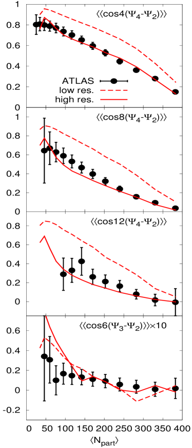
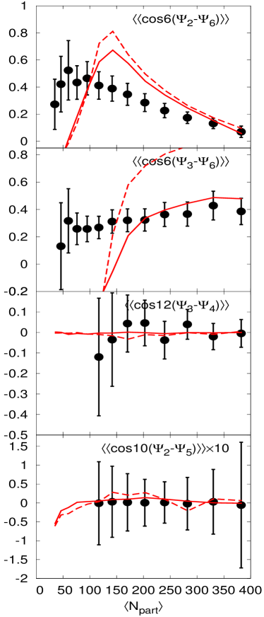
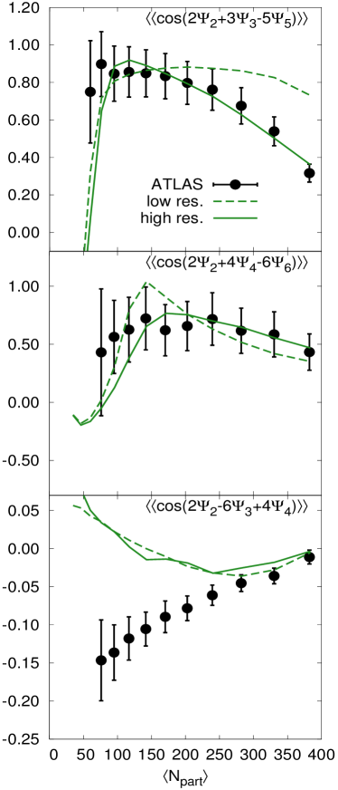
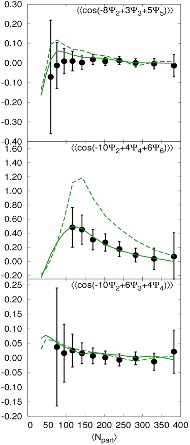
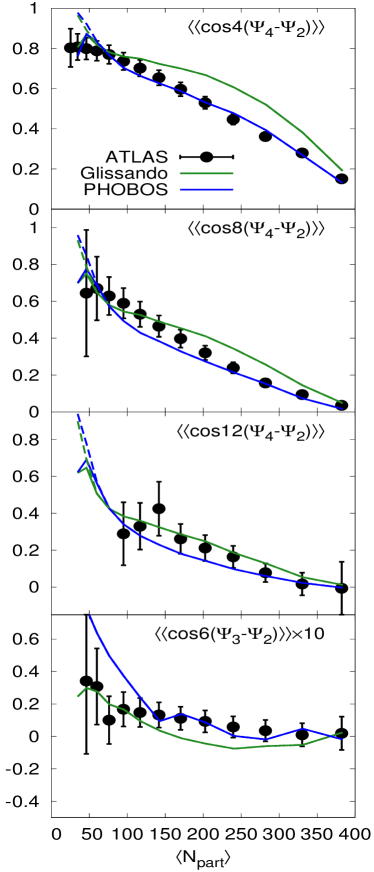
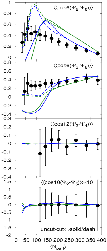
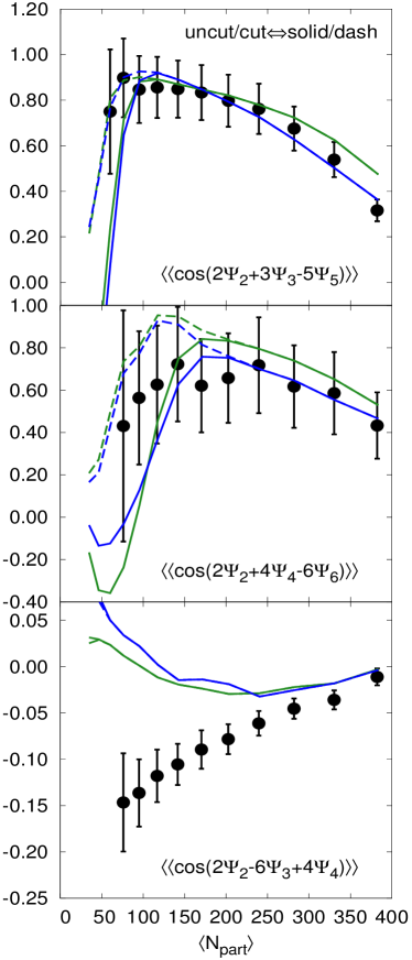
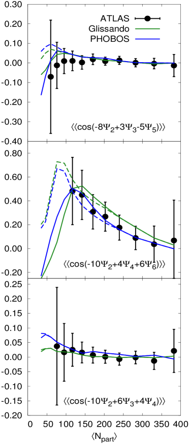
Inspecting these correlations, we make the following observations. First, many of the most important correlation functions are reasonably reproduced, at least if the high resolution limit is used. The agreement with the low resolution limit is not as good. The ambiguities in the measurement can be avoided by taking definite moments as in eq. (20) Bhalerao et al. (2011b). Examining the definitions of the high and low resolution limits (Eqs. 18 and 19), we see that the difference between the two measurements can be best quantified by measuring the probability distribution $P(v_{n})$ Aad et al. (2013), or the moments of this distribution Alver et al. (2010b), e.g. for $v_{2}$

$$(v_{2}\{2\})^{2}\equiv\left\langle v_{2}^{2}\right\rangle\quad\mbox{and}\quad(v_{2}\{4\})^{4}\equiv-\left[\left\langle v_{2}^{4}\right\rangle-2\left\langle v_{2}^{2}\right\rangle\right]\,.$$ (24)

It is then a separate and important question whether the response formalism outlined here can reproduce these probability distributions. This will be addressed in future work.

There are a few correlations which are seemingly not well reproduced even in the high resolution limit. First, one could hope for better agreement with the correlations involving $\Psi_{6}$ such as $\cos(6\Psi_{3}-6\Psi_{6})$ and $\cos(6\Psi_{2}-6\Psi_{6})$. $v_{6}$ is a relatively high harmonic, and viscous corrections are not in perfect control in peripheral collisions Teaney and Yan (2013). This is clearly evident in Fig. 5 which estimates the contributions of higher order viscous corrections to the distribution function (see above). For the $\Psi_{6}$-correlations (and no others), these corrections are large in peripheral collisions.

The most troubling correlation function, which is not qualitatively reproduced by the response formulation, is $\cos(2\Psi_{2}-6\Psi_{3}+4\Psi_{4})$. It is possible that that this discrepancy stems from an underestimate of the mixing of $v_{1}$ with other modes, which naturally mixes $v_{4}$ with $v_{3}$. Indeed, a preliminary analysis suggests that this correlation is closely related to the transverse shift from the geometrical center to the center of participants. The $2,3,4$ correlation is qualitatively reproduced by event-by-event hydrodynamics Qiu and Heinz (2012).

It is important and instructive to understand the hydrodynamic origin of the correlations presented in these figures. This is best understood by examining the linear and non-linear contributions separately. Fig. 7(a) and (b) illustrate this decomposition with the correlations $\left\langle\cos(4(\Psi_{2}-\Psi_{4}))\right\rangle$ and $\left\langle\cos(2\Psi_{2}+3\Psi_{3}-5\Psi_{5})\right\rangle$ respectively. For definiteness, we study the 2,3,5 combination shown in Fig. 7(b). The naive expectation of the Glauber model (where $v_{n}$ is proportional to the $n-$th order moment based eccentricity) is shown by the dotted line, and has the wrong sign. In the naive approach the observed correlation between the event plane angles $2,3,5$ arises from the correlations between the angles associated with the corresponding moment based eccentricities.

Figure 7: The separate contributions of the linear and non-linear response to a two-plane correlation, $\left\langle\cos(4\Psi_{4}-4\Psi_{2})\right\rangle$, and a three-plane correlation, $\left\langle\cos(2\Psi_{2}+3\Psi_{3}-5\Psi_{5})\right\rangle$. The dashed lines show the naive Glauber expectation (see text). The data is from Ref. Collaboration (May, 2012).

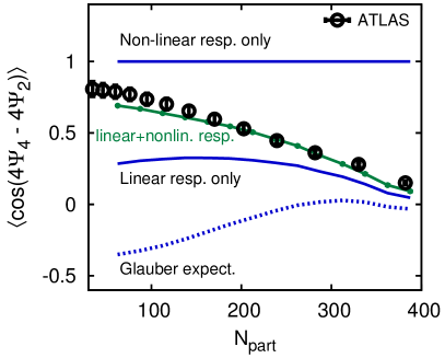
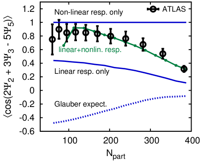
In the current work the $v_{5}$ is produced through a combination of the linear and non-linear response.

• In linear response, $v_{5}$ is proportional to the $5$-th cumulant $\epsilon_{5}$, and the correlation between the event plane angles $\Psi_{2},\Psi_{3},\Psi_{5}$ reflects the initial state correlation between the associated cumulant angles, $\Phi_{2},\Phi_{3},\Phi_{5}$. The predictions of linear response are shown in Fig. 7, and fail to reproduce the observed correlations in non-central collisions.

• In non-linear response, $v_{5}$ is determined through the mode mixing of $v_{2}$ and $v_{3}$. If $v_{5}$ was determined entirely by this mechanism, the $\Psi_{5}$ event plane would be entirely determined by $\Psi_{2}$ and $\Psi_{3}$, leading to a perfect $2,3,5$ correlation. This prediction of non-linear response is also shown in Fig. 7.

In general, $v_{5}$ is determined by a weighted average of the linear and non-linear response curves. The relative size of these two contributions is determined by viscous hydrodynamics which predicts the magnitude of these response coefficients as a function of centrality. Evidently, hydrodynamics and the response formalism reproduces the centrality dependence of the observed correlation functions. It is satisfying to see how the data transition between the linear response curves in central collisions, and the non-linear response curves in peripheral collisions.

Finally, we conclude by discussing the importance of higher order terms in the response formalism. First, we have neglected the third order mixing of harmonics. The most important third order term is proportional to ${\mathcal{E}}_{2}^{3}$, and we have found that this term is small compared to the ${\mathcal{E}}_{3}^{2}$ and ${\mathcal{E}}_{2}{\mathcal{E}}_{4}$ terms. Thus, the response formalism seems to converge, and including the mixing of higher harmonics will not change the results of this study significantly.

In the future it will be important to characterize the fluctuations around the response formalism. For any given initial state characterized by a few macroscopic cumulants such as ${\mathcal{E}}_{2},{\mathcal{E}}_{3},{\mathcal{E}}_{4}\ldots$, the observed $v_{n}$ will on average be given by the response formalism. However, additional fluctuations (which leave the macroscopic cumulants fixed) will reduce the perfect correlation between $v_{2},v_{3},v_{4},\ldots$ and the predictions of non-linear response. Thus, in general, the response formalism will overestimate the strength of the correlations that are observed. Ideally, the fluctuations around the response formalism can be parametrized by universal Gaussian noise, which will be independent of the microscopic details of the initial state. The study of fluctuations around the response formalism is left for future work.

Acknowledgments:

We thank J. Y. Ollitrault, Z. Qiu, U. Heinz, J. Jia, and S. Mohapatra for many constructive and insightful comments. D. Teaney is a RIKEN-RBRC fellow. This work is supported by the Department of Energy, DE-FG-02-08ER4154. Li Yan is also funded by the European Research Council under the Advanced Investigator Grant ERC-AD-267258.

References

- Heinz and Snellings (2013) Ulrich W Heinz and Raimond Snellings, “Collective flow and viscosity in relativistic heavy-ion collisions,” (2013), arXiv:1301.2826 [nucl-th] .
- Hippolyte and Rischke (2013) Boris Hippolyte and Dirk H. Rischke, “Global variables and correlations: Summary of the results presented at the Quark Matter 2012 conference,” Nucl.Phys. A904-905, 318c–325c (2013), arXiv:1211.6714 [nucl-ex] .
- Teaney (2009) Derek A. Teaney, “Viscous Hydrodynamics and the Quark Gluon Plasma,” (2009), invited review for ’Quark Gluon Plasma 4’. Editors: R.C. Hwa and X.N. Wang, World Scientific, Singapore., arXiv:0905.2433 [nucl-th] .
- Alver and Roland (2010) B. Alver and G. Roland, “Collision geometry fluctuations and triangular flow in heavy-ion collisions,” Phys.Rev. C81, 054905 (2010), arXiv:1003.0194 [nucl-th] .
- Qiu and Heinz (2011) Zhi Qiu and Ulrich W. Heinz, “Event-by-event shape and flow fluctuations of relativistic heavy-ion collision fireballs,” Phys.Rev. C84, 024911 (2011), arXiv:1104.0650 [nucl-th] .
- Gardim et al. (2012) Fernando G. Gardim, Frederique Grassi, Matthew Luzum, and Jean-Yves Ollitrault, “Mapping the hydrodynamic response to the initial geometry in heavy-ion collisions,” Phys.Rev. C85, 024908 (2012), arXiv:1111.6538 [nucl-th] .
- Borghini and Ollitrault (2006) Nicolas Borghini and Jean-Yves Ollitrault, “Momentum spectra, anisotropic flow, and ideal fluids,” Phys.Lett. B642, 227–231 (2006), arXiv:nucl-th/0506045 [nucl-th] .
- Floerchinger et al. (2013) Stefan Floerchinger, Urs Achim Wiedemann, Andrea Beraudo, Luca Del Zanna, Gabriele Inghirami, et al., “How (non-) linear is the hydrodynamics of heavy ion collisions?” (2013), arXiv:1312.5482 [hep-ph] .
- Teaney and Yan (2012) Derek Teaney and Li Yan, “Non linearities in the harmonic spectrum of heavy ion collisions with ideal and viscous hydrodynamics,” Phys.Rev. C86, 044908 (2012), arXiv:1206.1905 [nucl-th] .
- Collaboration (May, 2012) The ATLAS Collaboration, “Measurement of reaction plane correlations in Pb-Pb collisions at =2.76 TeV,” (May, 2012), ATLAS-CONF-2012-049. See also https://cdsweb.cern.ch/record/1451882.
- Bilandzic (2013) Ante Bilandzic (ALICE Collaboration), “Anisotropic flow measured from multi-particle azimuthal correlations for Pb-Pb collisions at 2.76 TeV by ALICE at the LHC,” Nucl.Phys.A904-905 2013, 515c–518c (2013), arXiv:1210.6222 [nucl-ex] .
- Luzum and Ollitrault (2013) Matthew Luzum and Jean-Yves Ollitrault, “The event-plane method is obsolete,” Phys.Rev. C87, 044907 (2013), arXiv:1209.2323 [nucl-ex] .
- Qiu and Heinz (2012) Zhi Qiu and Ulrich Heinz, “Hydrodynamic event-plane correlations in Pb+Pb collisions at ATeV,” Phys.Lett. B717, 261–265 (2012), arXiv:1208.1200 [nucl-th] .
- Bhalerao et al. (2013) Rajeev S. Bhalerao, Jean-Yves Ollitrault, and Subrata Pal, “Event-plane correlators,” (2013), arXiv:1307.0980 [nucl-th] .
- Gale et al. (2013) Charles Gale, Sangyong Jeon, Bjorn Schenke, Prithwish Tribedy, and Raju Venugopalan, “Event-by-event anisotropic flow in heavy-ion collisions from combined Yang-Mills and viscous fluid dynamics,” Phys.Rev.Lett. 110, 012302 (2013), arXiv:1209.6330 [nucl-th] .
- Broniowski et al. (2009) Wojciech Broniowski, Maciej Rybczynski, and Piotr Bozek, “GLISSANDO: Glauber initial-state simulation and more..” Comput.Phys.Commun. 180, 69–83 (2009), arXiv:0710.5731 [nucl-th] .
- Alver et al. (2008) B. Alver, M. Baker, C. Loizides, and P. Steinberg, “The PHOBOS Glauber Monte Carlo,” (2008), arXiv:0805.4411 [nucl-ex] .
- Floerchinger and Wiedemann (2013a) Stefan Floerchinger and Urs Achim Wiedemann, “Mode-by-mode fluid dynamics for relativistic heavy ion collisions,” (2013a), arXiv:1307.3453 .
- Floerchinger and Wiedemann (2013b) Stefan Floerchinger and Urs Achim Wiedemann, “Kinetic freeze-out, particle spectra and harmonic flow coefficients from mode-by-mode hydrodynamics,” (2013b), arXiv:1311.7613 [hep-ph] .
- Yan (2013) Li Yan, “A Hydrodynamic Analysis of Collective Flow in Heavy-Ion Collisions,” Ph.D. thesis, Stony Brook University (2013).
- Dusling et al. (2010) Kevin Dusling, Guy D. Moore, and Derek Teaney, “Radiative energy loss and v(2) spectra for viscous hydrodynamics,” Phys.Rev. C81, 034907 (2010), arXiv:0909.0754 [nucl-th] .
- Laine and Schroder (2006) Mikko Laine and York Schroder, “Quark mass thresholds in QCD thermodynamics,” Phys.Rev. D73, 085009 (2006), arXiv:hep-ph/0603048 [hep-ph] .
- Luzum and Romatschke (2008) Matthew Luzum and Paul Romatschke, “Conformal Relativistic Viscous Hydrodynamics: Applications to RHIC results at ,” Phys. Rev. C78, 034915 (2008), arXiv:0804.4015 [nucl-th] .
- Teaney and Yan (2013) Derek Teaney and Li Yan, “Second order viscous corrections to the harmonic spectrum in heavy ion collisions,” (2013), arXiv:1304.3753 [nucl-th] .
- Bhalerao et al. (2011a) Rajeev S. Bhalerao, Matthew Luzum, and Jean-Yves Ollitrault, “Understanding anisotropy generated by fluctuations in heavy-ion collisions,” Phys.Rev. C84, 054901 (2011a), arXiv:1107.5485 [nucl-th] .
- Bhalerao et al. (2011b) Rajeev S. Bhalerao, Matthew Luzum, and Jean-Yves Ollitrault, “Determining initial-state fluctuations from flow measurements in heavy-ion collisions,” Phys.Rev. C84, 034910 (2011b), arXiv:1104.4740 [nucl-th] .
- Alver et al. (2010a) Burak Han Alver, Clement Gombeaud, Matthew Luzum, and Jean-Yves Ollitrault, “Triangular flow in hydrodynamics and transport theory,” Phys.Rev. C82, 034913 (2010a), arXiv:1007.5469 [nucl-th] .
- Aad et al. (2013) Georges Aad et al. (ATLAS Collaboration), “Measurement of the distributions of event-by-event flow harmonics in lead–lead collisions at =2.76 TeV with the ATLAS detector at the LHC,” (2013), arXiv:1305.2942 [hep-ex] .
- Alver et al. (2010b) B. Alver et al. (PHOBOS Collaboration), “Event-by-Event Fluctuations of Azimuthal Particle Anisotropy in Au + Au Collisions at GeV,” Phys.Rev.Lett. 104, 142301 (2010b), arXiv:nucl-ex/0702036 [nucl-ex] .