Analysis and Simulation of the Three-Component Model of HIV Dynamics

Abstract

Mathematical modeling of biological systems is crucial to effectively and efficiently developing treatments for medical conditions that plague humanity. Often, systems of ordinary differential equations are a traditional tool used to describe the spread of disease within the body. We consider the dynamics of the Human Immunodeficiency Virus (HIV) in vivo during the initial stages of infection. In particular, we examine the well-known three-component model and prove the existence, uniqueness, and boundedness of solutions. Furthermore, we prove that solutions remain biologically meaningful, i.e., are positivity preserving, and perform a thorough, local stability analysis for the equilibrium states of the system. Finally, we incorporate random coefficients within the model and obtain numerical results to predict the probability of infection given the transmission of the virus to a new individual.

1 Introduction

The human body has been studied for hundreds of years, and the knowledge accumulated to date includes intricate molecular level mechanisms that determine the ways in which a virus may infect cells and replicate. This information is necessary to develop treatments for maladies ranging from Hepatitis to the Human Immunodeficiency Virus (HIV) and Acquired Immunodeficiency Syndrome (AIDS). An understanding of the accumulation of millions of these interactions across a timescale of medical relevance permits the creation of better treatment methods. As recently as fifty years ago, this could only be done via experiment and repeated trials. Today, through the advent of high speed computing, viral kinetics can be simulated using mathematical models. Hence, one can utilize our current understanding of molecular and cellular dynamics, describe them in mathematical terms, and simulate interactions within the body to examine the course of a virus from initial transmission to a long-term infection. In this paper we will consider the three-component model (3CM) for HIV [BCN, KW, NB, DS, NM]. We will study the infection within a single human host using this system of differential equations, analyze the resulting dynamics of the model, and simulate the behavior of solutions.

Generally speaking, HIV infection without the inclusion of anti-retroviral therapy (ART) is described by a number of distinct phases [PerelsonSIAM]. In the early stages of HIV infection, symptomatic primary infection yields high concentrations of virions within an individual’s blood or tissue. After several weeks, the flu-like symptoms disappear and the viral density then declines rapidly within several days. This corresponds to an increase in the amount of cytotoxic T lymphocytes and the subsequent appearance of anti-HIV antibodies in the blood. For years afterward, the viral concentration deviates very little from this low level and the host typically does not exhibit symptoms of HIV infection, but the concentration of CD$\displaystyle 4^{+}$ T cells measured in blood slowly declines. Such a period can last as long as $\displaystyle 10$ years. Ultimately, the viral load increases, the T-cell count drops below $\displaystyle 200$ cells per $\displaystyle\mu L$ of blood, and the symptoms of AIDS appear.

Within the current study, we will focus on the initial stages of transmission and infection, detailing the quick rise of the virion population within the body and the noted decrease in the number of CD$\displaystyle 4^{+}$ T-cells. Mathematical models for HIV population dynamics have been used to understand the basic mechanisms involved in the evolution of the infection at the microscopic level and to ascertain the effects of anti-retroviral therapy [PerelsonSIAM, PKdB]. To date, deterministic models of HIV dynamics have included at least two components: the population of uninfected CD$\displaystyle 4^{+}$ T-cells and the density of virus-producing cells. However, in the construction of a model for early HIV dynamics one may consider several components as populations within the the blood or lymphatic tissue, including latently-infected CD$\displaystyle 4^{+}$ T-cells, macrophages, and actively-producing infected macrophages. As previously described, the time-dependent changes in the cytotoxic T-lymphocytes which directly attack virus producing CD$\displaystyle 4^{+}$ T-cells could also be included within a model, but as previously stated, this may not have significant impact within the earliest stage of infection. Similarly, effects of time delays between infection of T-cells and active production of virions, or multiple compartment models, which couple the dynamics of multiple infected regions of the body, may also play a role in later stages, but are omitted from the current study. Nevertheless, some authors have found it useful to consider simple models which include only the density of virions, the uninfected CD$\displaystyle 4^{+}$ T-cell population, and one class of (actively-productive) infected CD$\displaystyle 4^{+}$ T-cells. This gives rise to three-component models as in [BCN, KW, NB]. We emphasize that the current article focuses only on the early period, up to a couple of months after infection, and does not study the later progression to the acquired immune deficiency syndrome (AIDS) which may follow without the use of anti-retroviral therapy.

2 Background and Derivation of Mathematical Model

The general principle behind any sort of mathematical model is to examine closely the interactions between the quantities being analyzed. We begin with a small number of initial axioms, and then follow the implications thoroughly to their conclusion. As a basis for our model, we utilize a general biological understanding of HIV dynamics, including infection, replication, and clearance.

In this section we describe the three-component model that has been widely used in the study of HIV. There are many biological operators involved in the interaction between HIV and cells within the human body. The first group is a subset of the population of lymphocytes, which in turn are a type of white blood cell. This subset is known as CD$\displaystyle 4^{+}$ T-cells, or helper T-cells. These T-cells have a variety of functions, including secreting substances that stimulate the immune system, in addition to acting as memory agents and regulating the immune response. In short, CD4+ T-cells detect and direct immune system responses to invading bacteria and viruses. Without them, the body significantly suffers from opportunistic infections that are greater in severity and duration than they would be if the CD4+ T-cells were otherwise not present. HIV, which refers in this case to the virus, not the disease or symptoms associated with it, is a retrovirus that infects helper T-cells. The virus, which is significantly smaller than the T-cell ($\displaystyle 120$ nm in diameter compared with $\displaystyle 7$ $\displaystyle\mu$m in diameter, respectively), breaches the cell wall and transports its RNA into the T-cell nucleus, where it may remain dormant for a time. Upon activation, the T-cell ceases its function as part of the immune system and instead produces additional copies of HIV. These infected T-cells, along with the healthy T-cells and free floating HIV, are the populations with which we are concerned, and will appear within the mathematical model.

The second aspect of the model’s creation involves incorporating the interactions between these populations and deriving their corresponding mathematical representation. Healthy T-cells are created from stem cells in the bone marrow, and mature in the thymus. While production of T-cells does decrease with the aging of the human body, we shall consider it to be a constant process for two reasons. First, there is no known method other than this production that can affect T-cell creation, and second, the time scale of interest within the model is sufficiently small to consider the T-cell production rate as constant. When considering removal of these cells, we note that T-cells do age and, in time, expire. Within the model, we assume that each T-cell functions for roughly the same amount of time, and thus, the death rate does not vary over the entire population. Instead, we assume the overall number of T-cells lost in a group over a certain period of time is proportional to the number of T-cells within the group. The other mechanism through which the population of healthy T-cells may decrease is via infection. In considering such effects, we utilize an interaction term that arises from the widely-used “mass action principle” to describe the transfer between populations when the virus infects healthy T-cells. This mass action term represents the idea that the rate of interaction, or infection, is directly proportional to the product of the participating populations, namely those of virions (or virus particles) and healthy T-cells. This completes the interactions for the healthy T-cells. We note that the only way to increase the population of infected T-cells is through HIV infection. Thus, our model will contain the same mass action term to describe the removal of the healthy T-cells and the addition of infected T-cells. Similar to the healthy T-cells, infected T-cells die-off or are cleared by the immune system at a rate proportional to the size of their current population. The virus, while produced from the infected T-cells, does not cause the destruction of infected T-cells. Thus, such a transition is not included within the model.

While the virus production rate does differ from cell to cell, we can assume that the aggregate rate is proportional to the population of infected T-cells. This is the only mechanism by which the virus can be created. In contrast, there are two manners in which the virus can be removed, or cleared, from the body. The first is through viral infection of T-cells. The act of infecting a healthy T-cell must technically remove a virus particle from the population of viruses that can infect further T-cells. However, when considering the overall population quantities, the amount of viruses lost this way is minute compared to other methods of creation and destruction. Hence, we will omit this mechanism. The second method of removal is known as viral clearance. It is the removal by the body of individual virus particles, and is performed at a rate proportional to the current amount of virus particles within the body.

We denote by $\displaystyle T$, $\displaystyle I$, and $\displaystyle V$, the number of healthy T-cells, infected T-cells and virions respectively. Based on the biological description above we have the following system of three ODEs:

(3CM) $$\left\{\begin{aligned} \frac{dT}{dt}&=\lambda-\mu T-kTV\\ \frac{dI}{dt}&=kTV-\delta I\\ \frac{dV}{dt}&=pI-cV.\end{aligned}\right.$$

The parameters $\displaystyle\lambda,\mu,k,\delta,p,c$ play an important role in our later results on viral persistence. Based on biological considerations we assume that these constants are positive. Table 2.1 shows typical values for these constants and the corresponding units. The values are the average values of these parameters from [SCCDHP].

Parameter	Biological Process	Minimum	Mean Value	Maximum	Units
$\displaystyle\lambda$	T-cell growth rate	$\displaystyle 0.043$	$\displaystyle 0.1089$	$\displaystyle 0.2$	$\displaystyle\mu L^{-1}$ day-1
$\displaystyle\mu$	T-cell death rate	$\displaystyle 0.0043$	$\displaystyle 0.01089$	$\displaystyle 0.02$	day-1
$\displaystyle k$	Infection rate	$\displaystyle 1.9\times 10^{-4}$	$\displaystyle 1.179\times 10^{-3}$	$\displaystyle 4.8\times 10^{-3}$	$\displaystyle\mu L$ day-1
$\displaystyle\delta$	Infected T-cell death rate	$\displaystyle 0.13$	$\displaystyle 0.3660$	$\displaystyle 0.8$	day-1
$\displaystyle p$	Virus production rate	$\displaystyle 98$	$\displaystyle 1.427\times 10^{3}$	$\displaystyle 7.1\times 10^{3}$	day-1
$\displaystyle c$	Viral clearance rate	$\displaystyle 3$	$\displaystyle 3$	$\displaystyle 3$	day-1

Table 2.1: Parameter values for (3CM) as observed in [SCCDHP]

The diagram (Fig 2.1) provides a brief visual representation of the mechanisms which govern the system of differential equations. We see each of the populations within a circle, while the arrows running to and from each circle describe their respective interaction.

Fig. 2.1: Illustration of 3CM

3 Mathematical Analysis

We now answer some fundamental questions about 3CM. In particular we will show that solutions to 3CM exist for all positive time, and are unique. Later we will show that the solution converge to one of two possible steady-states and that the solutions to 3CM remain positive given positive initial conditions. This last property is important since it shows that the model is biologically relevant.

3.1 Properties of Solutions

The first step in examining (3CM) is to prove that a solution to the initial-value problem does, in fact, exist, and that this solution is unique.

Theorem 1.

Let $\displaystyle T_{0},I_{0},V_{0}\in\mathbb{R}$ be given. There exists $\displaystyle t_{0}>0$ and continuously differentiable functions $\displaystyle T,I,V:[0,t_{0})\to\mathbb{R}$ such that the ordered triple $\displaystyle(T,I,V)$ satisfies (3CM) and $\displaystyle(T,I,V)(0)=(T_{0},I_{0},V_{0})$.

Proof.

To prove the result, we utilize the classical Picard-Lindelöf Theorem (cf. [Bartle]). Since the system of ODEs is autonomous, it suffices to show that the function $\displaystyle f:\mathbb{R}^{3}\to\mathbb{R}^{3}$ defined by

$$f(y)=\begin{bmatrix}\lambda-\mu y_{1}-ky_{1}y_{3}\\ ky_{1}y_{3}-\delta y_{2}\\ py_{2}-cy_{3}\end{bmatrix}$$

is locally Lipschitz in its $\displaystyle y$ argument. In fact, it is enough to notice that the Jacobian matrix

$$\nabla f(y)=\begin{bmatrix}-\mu-ky_{3}&0&-ky_{1}\\ ky_{3}&-\delta&ky_{1}\\ 0&p&-c\end{bmatrix}$$

is linear in $\displaystyle y$ and therefore locally bounded for every $\displaystyle y\in\mathbb{R}^{3}$. Hence, $\displaystyle f$ has a continuous, bounded derivative on any compact subset of $\displaystyle\mathbb{R}^{3}$ and so $\displaystyle f$ is locally Lipschitz in $\displaystyle y$. By the Picard- Lindelöf Theorem, there exists a unique solution, $\displaystyle y(t)$, to the ordinary differential equation $\displaystyle y^{\prime}(t)=f(y(t))$ on $\displaystyle[0,t_{0}]$ for some time $\displaystyle t_{0}>0$. ∎

Additionally, we may show that for positive initial data, solutions remain positive as long as they exist. A fortunate byproduct of this result is that the solutions are also bounded.

Theorem 2 (Boundedness and Positivity).

Assume the initial conditions of (3CM) satisfy $\displaystyle T_{0}>0$, $\displaystyle I_{0}>0$, and $\displaystyle V_{0}>0$. If the unique solution provided by Theorem 1 exists on the interval $\displaystyle[0,t_{0}]$ for some $\displaystyle t_{0}>0$, then the functions $\displaystyle T(t),I(t),$ and $\displaystyle V(t)$ will be bounded and remain positive for all $\displaystyle t\in[0,t_{0}]$.

Proof.

We assume that $\displaystyle T(t)$, $\displaystyle I(t)$, and $\displaystyle V(t)$ initially have positive values. From the previous theorem, there exists a $\displaystyle t^{*}$ such that the solution exists on $\displaystyle[0,t^{*}]$. Let us denote by $\displaystyle T^{*}$ the largest time for which all populations remain positive, or more precisely

$$T^{*}=\sup\{t\in[0,t^{*}]:T(s),I(s),V(s)>0\ \mbox{for all}\ s\in[0,t]\}.$$

Then on the interval $\displaystyle[0,T^{*}]$ we can make estimate the population values.

Recall that all constants in the system are positive. Using this and the positivity of solutions on $\displaystyle[0,T^{*}]$, we can place lower bounds on $\displaystyle\frac{dI}{dt}$ and $\displaystyle\frac{dV}{dt}$ since

$$\frac{dI}{dt}=kTV-\delta I\geq-\delta I$$

and

$$\frac{dV}{dt}=pI-cV\geq-cV.$$

Using an integrating factor, we rewrite these differential inequalities to find

$$I(t)\geq I(0)e^{-\delta t}>0$$

and

$$V(t)\geq V(0)e^{-ct}>0$$

for $\displaystyle t\in[0,T^{*}]$. Similarly, we can place an upper bound on $\displaystyle\frac{dT}{dt}$ so that

$$\frac{dT}{dt}=\lambda-\mu T-kTV\leq\lambda.$$

Solving for $\displaystyle T$ yields

$$T(t)\leq T(0)+\lambda t\leq C_{1}(1+t).$$

where the constant $\displaystyle C_{1}$ satisfies $\displaystyle C_{1}\geq\max\{\lambda,T(0)\}$. We can sum the equations for $\displaystyle\frac{dI}{dt}$ and $\displaystyle\frac{dV}{dt}$ and place bounds on this sum so that

$$\frac{d}{dt}(I+V)=kTV-\delta I+pI-cV\leq kTV+pI.$$

Recall that we have a bound on $\displaystyle T$, so we can substitute

$$\frac{d}{dt}(I+V)\leq kC_{1}(1+t)V+pI\leq C_{2}(1+t)(I+V)$$

where $\displaystyle C_{2}\geq\max\{kC_{1},p\}$. Solving the differential equation yields

$$(I+V)(t)\leq C_{3}e^{t^{2}}$$

for $\displaystyle t\in[0,T^{*}]$ where $\displaystyle C_{3}>0$ depends upon $\displaystyle C_{2}$, $\displaystyle I(0)$, and $\displaystyle V(0)$ only. Since $\displaystyle I(t)$ is positive, we can place an upper bound on $\displaystyle V$ by

$$C_{3}e^{t^{2}}\geq(I+V)(t)\geq V(t)$$

Additionally, since $\displaystyle V(t)$ is positive, it follows that $\displaystyle I(t)$ must be as well.

$$C_{3}e^{t^{2}}\geq(I+V)(t)\geq I(t)$$

With these bounds in place, we can now examine $\displaystyle T(t)$ and bound it from below using

$$\displaystyle\frac{dT}{dt} \displaystyle= \displaystyle\lambda-\mu T-kTV\geq-\mu T-kTV\geq-\mu T-kC_{3}e^{t^{2}}T$$

$$\displaystyle\geq \displaystyle-C_{4}(1+e^{t^{2}})T$$

for $\displaystyle t\in[0,T^{*}]$, where $\displaystyle C_{4}\geq\max\{\mu,kC_{3}\}$. Shifting that last term to the other side of the equation yields

$$\frac{dT}{dt}+C_{4}(1+e^{t^{2}})T\geq 0$$

Since we know

$$\frac{d}{dt}(T(t)+e^{C_{4}\int_{0}^{t}(1+e^{\tau^{2}}d\tau)})\geq 0,$$

then we find for $\displaystyle t\in[0,T^{*}]$

(1) $$T(t)\geq T(0)e^{-C_{4}\int_{0}^{t}(1+e^{\tau^{2}}d\tau)}>0.$$

Thus, the values of $\displaystyle T$, $\displaystyle I$, and $\displaystyle V$ stay strictly positive for all of $\displaystyle[0,T^{*}]$, including at time $\displaystyle T^{*}$. By continuity, there must exist a $\displaystyle t>T^{*}$ such that $\displaystyle T(t)$, $\displaystyle I(t)$, and $\displaystyle V(t)$ are still positive. This contradicts the definition of $\displaystyle T^{*}$, and shows that $\displaystyle T(t)$, $\displaystyle I(t)$, and $\displaystyle V(t)$ are strictly positive on the entire interval $\displaystyle[0,t^{*}]$. Additionally, on this same interval, all of the functions remain bounded, so the interval of existence can be extended further. In fact, the bounds on $\displaystyle T$, $\displaystyle I$, and $\displaystyle V$ derived above hold on any compact time interval. Thus, we may extend the time interval on which the solution exists to $\displaystyle[0,t_{0}]$ for any $\displaystyle t_{0}>0$ and from the above argument, the solutions remain both bounded and positive on $\displaystyle[0,t_{0}]$. ∎

With this, we have a general idea that the model is sound, and can say with certainty that it remains biologically valid as long as it began with biologically-reasonable (i.e, positive) data. This also shows that once infected, it is entirely possible that the virus may continue to exist beneath a detectable threshold without doing any damage. Finally, we remark that the bounds obtained above ensure the global existence of solutions.

Corollary 3.

Let $\displaystyle T_{0},I_{0},V_{0}>0$ be given. Then, for any $\displaystyle t_{0}>0$ there exist continuously differentiable functions $\displaystyle T,I,V:[0,t_{0}]\to\mathbb{R}$ such that the ordered triple $\displaystyle(T,I,V)$ satisfies (3CM) and $\displaystyle(T,I,V)(0)=(T_{0},I_{0},V_{0})$.

Thus, given positive initial data and any $\displaystyle t_{0}>0$, we can be certain that the solution stays both positive and bounded on the interval $\displaystyle[0,t_{0}]$.

3.2 Steady States

In order to fully understand the dynamics of the three component model, it is necessary to first determine values of equilibria. An equilibrium point is a constant solution of (3CM) so that if the system begins at such a value, it will remain there for all time. In other words, the populations are unchanging so the rate of change for each population is zero. Setting $\displaystyle\frac{dT}{dt}$,$\displaystyle\frac{dI}{dt}$, and $\displaystyle\frac{dV}{dt}$ equal to zero and solving the resulting equations for $\displaystyle T$, $\displaystyle I$, and $\displaystyle V$, we find that there exist exactly two equilibria. From a biological perspective, we can categorize these points to be when the HIV virus is either extinct from the body, i.e., $\displaystyle I=V=0$, or when the virus persists within the body $\displaystyle(I\neq 0,V\neq 0)$ as $\displaystyle t$ grows large.

We begin by solving for the nonlinear term in (3CM) and find $\displaystyle kTV=\delta I$. Additionally, the final equation implies $\displaystyle I=\frac{c}{p}V$. Using the latter equation to substitute for $\displaystyle I$, we find

$$kTV=\frac{\delta c}{p}V$$

or

$$V\left(kT-\frac{\delta c}{p}\right)=0.$$

Thus, either $\displaystyle V=0$ or $\displaystyle T=\frac{\delta c}{kp}$. In the former case, we find $\displaystyle I=0$ and thus $\displaystyle T=\frac{\lambda}{\mu}$. Hence, the ordered triplet

$$(T,I,V)=\left(\frac{\lambda}{\mu},0,0\right)$$

is an equilibrium solution known as viral extinction, since there are no virus particles or infected cells. We will refer to this point as $\displaystyle P_{E}$.

In the latter case, $\displaystyle T=\frac{c\delta}{pk}$, and substituting this value of $\displaystyle T$ into the first equation yields $\displaystyle V=\frac{p\lambda}{c\delta}-\frac{\mu}{k}$ and further substitution shows $\displaystyle I=\frac{\lambda}{\delta}-\frac{\mu c}{kp}$. Thus, a second equilibrium exists at the point

$$(T,I,V)=\left(\frac{c\delta}{pk},\frac{\lambda}{\delta}-\frac{\mu c}{kp},\frac{p\lambda}{c\delta}-\frac{\mu}{k}\right).$$

Since there are distinct presences of virus particles and infected T-cells, we refer to this point as viral persistence and abbreviate the point as $\displaystyle P_{P}$.

In terms of biology, we can say $\displaystyle P_{E}$ is the case in which an infection exists for a short period of time, then is removed from the body by natural means. The virus does not persist. The second case, where the system of equations tends to $\displaystyle P_{P}$, denotes that situation where the body is unable to clear the infection by itself. If this ends up being the case, than after a certain period of time, the Three Component Model loses its applicability as the infection takes a deeper hold on the body. More complex models, which consider latent infection, effects of macrophages, or cytotoxic immune response, are then required to describe the spread of HIV within the body and its development towards AIDS.

3.3 Stability Analysis

For linear ODEs, it is well-known that the stability properties depend only upon the eigenvalues of the system. However, our model (3CM) is nonlinear, and thus we must rely on linearization and a theorem of Hartman & Grobman [HartmanGrobman] to unify the local behavior of the linear and nonlinear systems.

We will investigate the local stability properties of these equilibria by approximating the nonlinear system of differential equations (3CM) with a linear system at the points $\displaystyle P_{E}$ and $\displaystyle P_{P}$. Then, we locally perturb the system from equilibrium and examine the resulting long time behavior. This is done by linearizing the system about each equilibria, using the Jacobian for (3CM)

$$J_{3CM}=\begin{bmatrix}-kV-\mu&0&-kT\\ kV&-\delta&kT\\ 0&p&-c.\end{bmatrix}$$

Then, by studying the linearized system

$$\dot{z}(t)=J_{3CM}(P)z(t)$$

we can investigate the stability of each equilibrium point $\displaystyle P=P_{E}$ and $\displaystyle P=P_{P}$. As we will see below, this property depends only on a single number, referred to as the basic reproduction number, $\displaystyle R$ given by

(2) $$R=\frac{kp\lambda}{c\delta\mu}.$$

We now prove two theorems that demonstrate the relationship between the value of $\displaystyle R$ and the local asymptotically stability of equilibria. These results imply that one can simply examine the value of $\displaystyle R$ to determine whether viral persistence or viral extinction occurs in the limit of the system as $\displaystyle t\to\infty$. This is a remarkable result that allows for the estimation of the persistence of HIV upon initial infection solely by Monte-Carlo simulations by generating different values of $\displaystyle R$, as in [TuckShip].

Theorem 4.

The viral extinction equilibrium $\displaystyle P_{E}$ given by

$$(T,I,V)=\left(\frac{\lambda}{\mu},0,0\right)$$

is locally asymptotically stable if and only if $\displaystyle R\leq 1$.

Proof.

We begin by computing $\displaystyle J_{3CM}(P_{E})$ and determining its corresponding eigenvalues, since these values are known to characterize the local asymptotic behavior of the associated linear system. Specifically, if every eigenvalue possesses negative real part, then the equilibrium point will be stable. On the other hand, if one or more of the eigenvalues possess positive real part, then small perturbations from equilibrium result in magnifications of those disturbances, and the unstable manifold is nontrivial. We remark that in the rare event that $\displaystyle R=1$, the equilibria $\displaystyle P_{E}$ and $\displaystyle P_{P}$ are identical. Hence, we’ll focus on the case in which $\displaystyle R<1$ since the asymptotic stability can been shown when $\displaystyle R=1$ by using a Lyapunov function [Korob] instead of an analysis of the linearized system.

Evaluating the Jacobian at $\displaystyle P_{E}=\left(\frac{\lambda}{\mu},0,0\right)$ results in

$$J_{3CM}(P_{E})=\begin{bmatrix}-\mu&0&-\frac{k\lambda}{\mu}\\[4.0pt] 0&-\delta&\frac{k\lambda}{\mu}\\[4.0pt] 0&p&-c\\ \end{bmatrix}$$

The corresponding characteristic equation can be written as

$$\det\left[x\mathbb{I}-J_{3CM}(P_{E})\right]=0$$

or

$$(x+\mu)\left((x+\delta)(x+c)-\frac{kp\lambda}{\mu}\right)=0.$$

Thus, $\displaystyle x=-\mu<0$ is one negative eigenvalue of the system, The remaining quadratic equation is

$$x^{2}+a_{1}x+a_{2}=0$$

where $\displaystyle a_{1}=c+\delta$ and $\displaystyle a_{2}=c\delta-\frac{kp\lambda}{\mu}$. Thus, the other eigenvalues are

$$x_{\pm}=\frac{-(c+\delta)\pm\sqrt{(c+\delta)^{2}-4(c\delta-\frac{kp\lambda}{\mu}})}{2}.$$

Since the first term under the square root is nonnegative, these eigenvalues have negative real part if and only if

$$4\left(c\delta-\frac{kp\lambda}{\mu}\right)>0$$

or

$$4c\delta(1-R)>0.$$

Since all parameters are positive, we see that all eigenvalues possess negative real part if and only if $\displaystyle R<1$. Thus, in this case the origin is a locally asymptotically stable equilibrium for the system

$$\dot{z}(t)=J_{3CM}(P_{E})z(t).$$

Finally, by the Hartman-Grobman Theorem, the asymptotic behavior of (3CM) is equivalent to that of this linear system for local perturbations, and the result follows. For a more detailed look at the transference of stability properties from linear to nonlinear systems of ordinary differential equations, see [Logan]. ∎

Now that $\displaystyle R$ has been incorporated within the stability analysis, we can rewrite the viral persistence equilibrium in terms of $\displaystyle R$, and notice that it possesses nonpositive population values for $\displaystyle R\leq 1$. Hence, it should not be surprising that solutions do not tend to this equilibrium for such values of $\displaystyle R$. However, as long as $\displaystyle R>1$, we find that viral persistence is stable.

Theorem 5.

The viral persistence equilibrium $\displaystyle P_{P}$ given by

$$(T,I,V)=\left(\frac{\lambda}{\mu R},\frac{\lambda}{\delta R}(R-1),\frac{\mu}{k}(R-1)\right)$$

is locally asymptotically stable if and only if $\displaystyle R>1$.

Proof.

The analysis for $\displaystyle P_{P}$ is similar to that of $\displaystyle P_{E}$. We first linearize (3CM) about $\displaystyle P_{P}$ and examine the characteristic equation. The Jacobian is slightly more complicated in this case, but it is given by

$$\begin{gathered}J_{3CM}(P_{P})=\begin{bmatrix}-k\left(\frac{p\lambda}{c\delta}-\frac{\mu}{k}\right)-\mu&&0&&-k\left(\frac{c\delta}{pk}\right)\\[4.0pt] k\left(\frac{p\lambda}{c\delta}-\frac{\mu}{k}\right)&&-\delta&&k\left(\frac{c\delta}{pk}\right)\\[4.0pt] 0&&p&&-c\\ \end{bmatrix}\\ =\begin{bmatrix}-\frac{k\lambda p}{c\delta}&&0&&-\frac{c\delta}{p}\\[4.0pt] \frac{k\lambda p}{c\delta}-\mu&&-\delta&&\frac{c\delta}{p}\\[4.0pt] 0&&p&&-c.\end{bmatrix}\end{gathered}$$

This results in the characteristic equation

$$\left(x+\frac{k\lambda p}{c\delta}\right)\biggl{(}(x+\delta)(x+c)-c\delta)\biggr{)}+\frac{c\delta}{p}\left({\frac{k\lambda p}{c\delta}-\mu}\right)p=0$$

with expanded form

$$x^{3}+a_{1}x^{2}+a_{2}x+a_{3}=0$$

where

$$\begin{gathered}a_{1}=c+\delta+\frac{k\lambda p}{c\delta}\\ a_{2}=\frac{k\lambda p}{\delta}+\frac{k\lambda p}{c}\\ a_{3}=k\lambda p-c\delta\mu.\end{gathered}$$

In the case of (3CM), it is possible to determine the signs of the solutions to this equation using a theorem of Routh and Hurwitz [Routh, Hurwitz]. According to the Routh-Hurwitz criteria, all roots of this cubic equation possess negative real part if and only if $\displaystyle a_{1},a_{2},a_{3}>0$ and $\displaystyle a_{1}a_{2}>a_{3}$. Hence, it is sufficient to show that $\displaystyle R>1$ if and only if the Routh-Hurwitz criteria are satisfied.

Let us first assume $\displaystyle R>1$. Then, $\displaystyle a_{3}=k\lambda p-c\delta\mu=c\delta\mu(R-1)>0$ and since all the coefficients in the system are positive, $\displaystyle a_{1},a_{2}>0$. Additionally,

$$a_{1}a_{2}=\left(c+\delta+\frac{k\lambda p}{c\delta}\right)\left(\frac{k\lambda p}{\delta}+\frac{k\lambda p}{c}\right)>c\cdot\frac{k\lambda p}{c}=k\lambda p>k\lambda p-c\delta\mu=a_{3}.$$

Thus, $\displaystyle R>1$ implies that $\displaystyle P_{P}$ is a locally asymptotically stable equilibrium. The other direction follows trivially since $\displaystyle a_{3}>0$ implies $\displaystyle R>1$. Hence, this is both a necessary and sufficient condition due to the form of $\displaystyle a_{3}$, and the proof is complete.

∎

Fig. 3.1: Graphs of solutions to (3CM) with illustrative coefficients. Parameter values yield either $\displaystyle R\leq 1$ (top) or, for those given in Table 2.1, $\displaystyle R>1$ (bottom). In the latter case, $\displaystyle R\approx 15$. Time is measured in days.

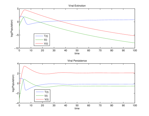
Our analysis reveals one very important fact about the overall system: for starting values sufficiently close to equilibrium, the long term behavior depends only on the value of $\displaystyle R$. If $\displaystyle R>1$ then the system tends towards an end state with a non-zero population of infected cells and virions (viral persistence), but if $\displaystyle R\leq 1$ then the final equilibrium is a state with no virus or infection (viral extinction). Figure 3.1 serves as an example that illustrates solutions in the two different cases given by Theorems 5 and 4. Finally, we also mention that global asymptotic stability of the equilibria can also be shown using a Lyapunov function as in [Korob].

Unfortunately, our analysis has been restricted to a deterministic model, and hence limited to only one possible solution, whereas in reality the systems under consideration may contain vast uncertainties, especially with regards to the parameters previously described. In the next section, we incorporate chance mechanisms for population coefficients in order to estimate the probability that a persistent infection develops upon an initial viral load being transmitted to a new host.

4 Numerical Simulations and the Probability of Persistence

Both mathematical and biological results support the idea that contact with HIV does not automatically imply the development of a persistent infection. Given factors such as the CD4+ T-cell growth rate, infection rate, and viral clearance rate, the theorems of the previous section display that it is possible to accurately predict the end viral state in the model. While this is very useful, it does not take into account the variability in parameter values amongst a group of individuals. To account for this, we now incorporate random coefficients for the early stages of HIV infection into the model and examine the resulting behavior. If these are introduced in a biologically meaningful fashion, we can estimate their contributions to the variability in the early time course of the viral load, which is not possible with the deterministic coefficients of the previous section. Furthermore, we can obtain predictions of the probability that HIV levels reach certain values as a function of time since initial infection. Such levels can correspond to thresholds in various tests for the detection of HIV in blood.

Another study [TuckShip] previously estimated the probability of viral persistence using the three-component model with random variable coefficients by using the results of Theorems 4 and 5. In this paper, the authors assumed that each random variable, except for $\displaystyle c$ which was assumed constant, possessed truncated normal distributions with the mean and standard deviation given by a clinical study of $\displaystyle 10$ infected patients [SCCDHP]. Upon sampling from these distributions, the authors computed the value of $\displaystyle R$ and used this to determine the asymptotic behavior of the system as $\displaystyle t\to\infty$, thereby avoiding the need to directly simulate the model itself. The results of their simulations estimated that the average probability of viral extinction was approximately $\displaystyle 1-7\%$.

There are a few issues with this approach that we plan to remedy in the current section. First and foremost, the validity of the model declines rapidly after several months [PerelsonSIAM, TuckShip] (approximately $\displaystyle 100$ days). Hence, determining viral persistence or extinction based solely on the asymptotic behavior of the system as $\displaystyle t\to\infty$ seems problematic. One can easily find solutions which possess large viral loads for several weeks, but eventually tend to extinction as $\displaystyle t\to\infty$. Another difficulty is that for certain coefficient values, the virus population in the model may stay quite small for the first few months after transmission, but then grow steadily to a persistent steady state over large times. These possible outcomes can be seen more clearly within Figure 4.1. Thus, instead of using the conditions $\displaystyle R\leq 1$ and $\displaystyle R>1$ (which provide information only about the behavior of (3CM) in the limit as $\displaystyle t\to\infty$) to determine whether or not a viral load has established a persistent infection, we will formulate and utilize new conditions which possess a finite time horizon. Since many standard tests for HIV currently display a threshold of detection of $\displaystyle 50$ virions per $\displaystyle\mu$L [RP, Rib], we will set this as the barrier for viral persistence at the end time of the model’s validity. Namely, the condition $\displaystyle V(100)\geq 50$ will represent viral persistence, while $\displaystyle V(100)<50$ will represent extinction.

Fig. 4.1: A log plot of the virion population is shown (left) for a choice of parameters resulting in $\displaystyle R=2.03$, yet the viral load remains small, around $\displaystyle 10^{-7}$ copies per $\displaystyle\mu$ L, up to time $\displaystyle t=60$. For larger times, however, the result of Theorem 5 must apply and hence the viral population rebounds and settles into equilibrium near $\displaystyle 10$ copies per $\displaystyle\mu$L by $\displaystyle t=600$ (left inset). A log plot of the virion population is shown (right) for a choice of parameters resulting in $\displaystyle R=0.74$, yet the viral load remains large, around $\displaystyle 10^{4}$ copies per $\displaystyle\mu$L up to time $\displaystyle t=60$. For larger times, however, the result of Theorem 4 must apply and hence the viral population sharply decreases to zero, with values around $\displaystyle 10^{-8}$ copies per $\displaystyle\mu$L by $\displaystyle t=600$ (right inset).

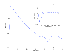
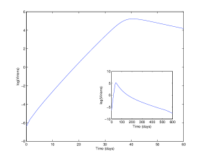
With these issues now in context, we perform a similar computational study to estimate the probability of persistence. To simulate the dynamics of the virus, we will employ a Monte-Carlo method along with a traditional Runge-Kutta solver to compute solutions of the corresponding systems of ordinary differential equations given by (3CM).

4.1 Sampling

We are interested in examining multiple definitions of viral persistence and allowing for a different parameter distribution than that of [TuckShip]. Hence, we consider two different cases. In the first case, we sample from truncated normal distributions as in [TuckShip] to determine the values of the random variable coefficients $\displaystyle\lambda,\mu,k,\delta$ and $\displaystyle p$, while keeping the parameter $\displaystyle c=3$ constant throughout. The probability of persistence is then estimated both using the time-asymptotic definition of viral persistence (i.e. $\displaystyle R>1$) and our new finite-time definition (i.e., $\displaystyle V(100)\geq 50$). In the second case, we investigate the influence of the distribution of parameters by sampling from uniform and triangular distributions, as previously performed for this system while considering the additional effects of viral mutation [RFP]. Here, viral promoters (i.e., those parameters which lead to large reproductive numbers) are sampled from uniform distributions, while viral inhibitors (in this case, death rates) are sampled from triangular distributions, data for both of which are taken from Table 2.1. In particular, the promoter $\displaystyle k$ is sampled from a uniform distribution over the interval $\displaystyle(1.9\times 10^{-4},4.8\times 10^{-3})$ $\displaystyle\mu$L/day similar to [RFP], and $\displaystyle p$ is sampled from another uniform distribution over the interval $\displaystyle(98,7100)$ day^-1. As in [BD], we assume an asymmetric triangular distribution $\displaystyle\mathrm{Tri}(0.0043,0.01089,0.02)$ day^-1 for $\displaystyle\mu$, the death rate of uninfected $\displaystyle T$-cells, where $\displaystyle 0.0043$ is the minimum value, $\displaystyle 0.01089$ is the peak (occurring at the mean recorded value in Table 2.1) and $\displaystyle 0.02$ is the maximum value. The growth parameter $\displaystyle\lambda$ is set to be $\displaystyle 10\mu$ as in [TuckShip], and the viral clearance rate $\displaystyle c$ is held constant at $\displaystyle 3$ as in [SCCDHP, TuckShip]. Finally, the death rate of infected $\displaystyle T$-cells, $\displaystyle\delta$ is sampled from another triangular distribution $\displaystyle\mathrm{Tri}(0.13,0.366,0.8)$ day^-1. Then, as before, the probability of persistence is estimated separately using the $\displaystyle R$ definition of viral persistence and our finite-time horizon.

Of course, because our condition depends upon solving the ODEs until a specific time, our results may now have a strong dependence on initial conditions. Thus, to generate a suitable range of initial data, we estimate the probabilities of persistence and extinction considering a variety of initial conditions. In particular, we choose values of $\displaystyle T_{0}$ between $\displaystyle 100-1000$ cells/$\displaystyle\mu$L, initial viral loads $\displaystyle V_{0}$ between $\displaystyle 100-500$ virions/$\displaystyle\mu$L, and fix the initial infected $\displaystyle T$-cell population at $\displaystyle 0$. These values are obtained from similar initial conditions of previous studies [PerelsonSIAM, PKdB].

4.2 Results

Fig. 4.2: Sample paths of the healthy T-cell, infected T-cell, and virion populations

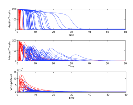
According to the described computational methods, $\displaystyle 500,000$ simulations were conducted to determine the probability of persistence of a specific infection. Sample paths of associated trials are displayed in Figure 4.2 and the results are summarized within Table 4.1. Notice that the proportion of trials within our simulation that resulted in $\displaystyle R\leq 1$ is much smaller - by a factor of ten or twenty - than those which resulted in viral populations less than $\displaystyle 50$ virions per $\displaystyle\mu$L approximately three months after the initial infection. Hence, a standard mathematical definition of extinction, namely $\displaystyle\lim_{t\to\infty}V(t)=0$ which (by Theorem 4) is equivalent to $\displaystyle R\leq 1$, appears to be insufficient to accurately describe the behavior of the viral population on the timescales of biological relevance, specifically during the time period up to a few months after initial infection. Instead, a more precise determination of viral extinction can be made by measuring whether the virus population will remain below the current detectable threshold of $\displaystyle 50$ virions per $\displaystyle\mu$L, and under this measure, the probability of extinction is much larger. As can be seen by Table 4.1, the probability of extinction by the former measure is only around $\displaystyle 1-2\%$, while the probability jumps to approximately $\displaystyle 8-15\%$ under the latter notion that we have proposed. In some types of transmission, such as passage of the disease from a mother to an unborn child or through needlesticks, this percentage is much closer to current estimates of the probability of extinction after initial infection than the criteria $\displaystyle R\leq 1$.

Parameter Distribution	$\displaystyle\mathbb{P}\left(R\leq 1\right)$	$\displaystyle\mathbb{P}\left(V(60)<50\frac{\mbox{copies}}{\mu\mbox{L}}\right)$
Truncated	0.0136	0.1510
Normal
Uniform &	0.0046	0.0859
Triangular

Table 4.1: Probabilities of virion extinction, using finite-time and time-asymptotic definitions of extinction, as well as different parameter distributions (truncated normal and uniform/triangular, respectively). A total of $\displaystyle 500,000$ trials were performed for each case; for the time-asymptotic probabilities, initial conditions were varied over 50 combinations, with $\displaystyle V(0)$ varying from 100-500 $\displaystyle\mu L^{-1}$ and $\displaystyle T(0)$ varying from 100-1000 $\displaystyle\mu L^{-1}$, and $\displaystyle I(0)$ set at 0. Hence, for each initial condition pair $\displaystyle(T(0),V(0))$, $\displaystyle 10,000$ trials were performed.

Based on the results of our simulations, which have been consolidated in Table 4.1, the probability of virus extinction using the finite time definition is significantly less than the extinction probability of the time-asymptotic definition by more than an order of magnitude. This result marks the distinction between the finite- and infinite-time results, and also alludes to the eventual breakdown of the model for $\displaystyle t>100$ as predicted results for (3CM) stray from clinical results [PerelsonSIAM, TuckShip].

Fig. 4.3: Average values of $\displaystyle\lambda$ over $\displaystyle 100,000$ draws using a truncated normal distribution (left), a uniform distribution (center), and a triangular distribution (right).

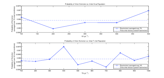
While the probability of viral extinction associated with the finite-time definition remained ten times higher than the corresponding asymptotic-time probability for each distribution, the extinction probabilities across the two distributions also varied by almost a factor of two. This demonstrates the system’s sensitivity to variations within the range of currently accepted values. In Figure 4.3 the difference between parameter distributions is shown, providing a description of how variations in parameter values can prompt a change in the model behavior.

Fig. 4.4: From parameters drawn from truncated normal distributions (as described in Section 4.1), these graphs show probabilities of virus extinction over varying initial conditions. $\displaystyle V(0)$ is varied from 100 to 500 while $\displaystyle T(0)$ is held constant (top), and $\displaystyle T(0)$ is varied from 100-1000 while $\displaystyle V(0)$ is held constant (bottom). $\displaystyle I(0)$ is kept fixed at $\displaystyle 0$ for all trials. Throughout all simulations, the variation in extinction probability remains small.

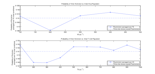
Lastly, it was expected that the initial conditions for T-cell and virus populations would have a significant impact on the probability of virus extinction, but based on our simulations this is not the case. As seen in Figures 4.4 and 4.5, for both distributions the initial conditions played little role: for each distribution, when averaged over the initial T-cell and initial virion conditions, the probability of persistence varied less than 5$\displaystyle\%$ from the mean value (averaged over all initial conditions). In addition, there is no clear pattern in the residuals of the probability of persistence of each initial condition relative to the overall probability, which suggests that the initial conditions have little to no effect to the disease’s end behavior. This same phenomena occurs in the asymptotic-time horizon definition of persistence, where the initial conditions are irrelevant to the probability of persistence of the virus.

Fig. 4.5: From parameters sampled from uniform and triangular distributions (as described in Section 4.1), these graphs show probabilities of virus extinction over varying initial conditions. $\displaystyle V(0)$ is varied from 100 to 500 while $\displaystyle T(0)$ is held constant (top), and $\displaystyle T(0)$ is varied from 100-1000 while $\displaystyle V(0)$ is held constant (bottom). $\displaystyle I(0)$ is kept fixed at $\displaystyle 0$ for all trials.

5 Conclusions

Three main accomplishments are noted within the current article. First, a local mathematical analysis was performed, and theorems were proved to justify the viability and utility of the three-component model. Second, the local asymptotic stability of steady states were proved and used to define mathematical notions for viral persistence and extinction. These conditions then inspire ODE-free simulations of the in-host viral dynamics merely be sampling from distributions describing the variation of parameters amongst a population of exposed individuals. Finally, we proposed alternative definitions for the notions of viral persistence and extinction, which possess a finite time horizon, rather than depending only upon the asymptotic limit as $\displaystyle t\to\infty$. Simulations were performed to measure the differences in these criteria and their dependence on the probability distribution of parameters. We note that the end viral population, $\displaystyle V(100)$, could be less than the threshold of detectability permitted by modern science much more often than predicted by the associated value of the reproduction ration $\displaystyle R$. This indicates that the methods used in [TuckShip] are not as accurate as could be hoped for. Hence, it should be clear that a full simulation of the model is required to obtain accurate results regarding the probability of developing a persistent infection.

With full simulation of the ordinary differential equations, we discovered that viral persistence occurred at a rate of roughly ten times that suggested in [TuckShip]. This proves rather conclusively the finite time and asymptotic limits conditions while related, do not yield identical predictions, and simulation is necessary to realize the full implications of the model. In reality, persistence has been estimated to occur at a rate of up to $\displaystyle 90\%$, if the virus is transmitted by blood transfusion, or around $\displaystyle 1\%$ if transmitted via sexual intercourse [Gray]. While [TuckShip] arrived at an average probability of persistence around $\displaystyle 93-99\%$ and we approximated this figure to be around $\displaystyle 85-92\%$, recall that these coefficients were drawn from a biased population of HIV-infected individuals because the data arose from people known to have already developed a persistent HIV infection. Additionally, the previous estimates already account for the probability of transmission within them, while our estimates of persistence and those of [TuckShip] specifically assume that transmission has occurred within a new host.

Stochastic models, such as in [TuckLC], that utilize Brownian motion to incorporate additional random effects stemming from factors outside of parameter estimation could provide additional improvement to our estimates of persistence, and this could be the goal of a future project. Due to the lack of mathematical tools to analyze stochastic differential equations, though, one would be forced to resort to a more computational framework, rather than a mathematical or asymptotic analysis, in order to glean information from the model. With the development of more descriptive models and more advanced analytical and computational tools, the probability of HIV persistence after initial infection can be estimated with even greater precision.

6 Acknowledgements

This work was completed under the direction of Prof. Mrinal Raghupathi and Prof. Stephen Pankavich, and submitted in partial fulfillment of MIDN Roemer’s Trident Scholar thesis requirement. Additionally, the authors were supported in part by National Science Foundation grants DMS-0908413 and DMS-1211667.