Toward Connecting Core-Collapse Supernova Theory with Observations: I. Shock revival in a 15 blue supergiant progenitor with SN 1987A energetics
Abstract
We study the evolution of the collapsing core of a 15 blue supergiant supernova progenitor from the core bounce until 1.5 seconds later. We present a sample of hydrodynamic models parameterized to match the explosion energetics of SN 1987A.
We find the spatial model dimensionality to be an important contributing factor in the explosion process. Compared to two-dimensional simulations, our three-dimensional models require lower neutrino luminosities to produce equally energetic explosions. We estimate that the convective engine in our models is % more efficient in three dimensions than in two dimensions. We propose that the greater efficiency of the convective engine found in three-dimensional simulations might be due to the larger surface-to-volume ratio of convective plumes, which aids in distributing energy deposited by neutrinos.
We do not find evidence of the standing accretion shock instability nor turbulence being a key factor in powering the explosion in our models. Instead, the analysis of the energy transport in the post-shock region reveals characteristics of penetrative convection. The explosion energy decreases dramatically once the resolution is inadequate to capture the morphology of convection on large scales. This shows that the role of dimensionality is secondary to correctly accounting for the basic physics of the explosion.
We also analyze information provided by particle tracers embedded in the flow, and find that the unbound material has relatively long residency times in two-dimensional models, while in three dimensions a significant fraction of the explosion energy is carried by particles with relatively short residency times.
Subject headings:
hydrodynamics — instabilities — shock waves — supernovae: generalCorresponding author: ]tplewa@fsu.edu
1. Introduction
There is substantial controversy over the importance of physics processes involved in core-collapse supernova (ccSN) explosions (see, e.g., Janka et al., 2012; Burrows, 2013, and references therein). One problem is a multitude of relevant processes which include hydrodynamics, gravity, nuclear equation of state, and neutrino-matter interactions. Despite much effort in the last four decades, no model accounting for these physics effects exists that consistently produces energetic ccSNe explosions for suitable progenitor models. Early theories of ccSNe explosions such as neutrino-driven convection (see, e.g., Burrows & Goshy, 1993; Janka & Mueller, 1996; Mezzacappa et al., 1998) and the more recent standing accretion shock instability (SASI) (Blondin et al., 2003) remain the centerpiece of computational core-collapse supernova studies.
The SASI mechanism has been discovered in the course of numerical simulations in the work by Blondin et al. (2003). Subsequent SASI studies included theoretical analysis (Laming, 2007; Foglizzo, 2009) and numerical investigations (Ohnishi et al., 2006; Blondin & Mezzacappa, 2007; Scheck et al., 2008). This shock instability is characterized by global, low order oscillations of the supernova shock which generate substantial non-radial flow in the post-shock region. These fluid motions result in increased residence times of the accreted material and possible increase the heating effect by neutrinos emitted by the nascent proto-neutron star.
Since SASI is only one of the participating processes, it is often times difficult to unambiguously quantify its contribution to the overall explosion process. Only recently has careful analysis been attempted to quantify the role of SASI and compare its contribution to the other major participating process of neutrino-driven convection. In particular, SASI may only be present in progenitors with higher masses when neutrino-driven convection might be suppressed by increased accretion rates (Müller et al., 2012, see also Bruenn et al. (2013)). Furthermore, the situation is additionally complicated by effects due to model dimensionality observed in some simulations (Murphy & Burrows, 2008; Nordhaus et al., 2010; Hanke et al., 2012; Dolence et al., 2013; Couch, 2013; Takiwaki et al., 2013). Those findings are, however, not confirmed by all studies (Janka et al., 2012). (In passing, we would like to note that is conceivable that the high frequency of SASI observations in two-dimensional simulations can be due to the assumed symmetry of such models. In either case, disentangling this kind of effects has not been attempted in a systematic manner.) There is also little known about the difference in the efficiency of convective heat transport between two and three dimensions, especially in the context of core-collapse supernovae. Although three-dimensional ccSNe explosion models have been available for some time (see, for example, Fryer & Warren, 2002), no systematic study aimed at comparing the convection efficiency between two and three dimensions exists.
In this work, we investigate the energetic explosions of a post-collapse WPE15 model of Bruenn (1993) in one, two, and three spatial dimensions. This model has been used extensively in the past by Kifonidis and his collaborators (Kifonidis et al., 2003, 2006; Gawryszczak et al., 2010, see also Wongwathanarat et al. (2013)), mainly in application to post-explosion mixing of nucleosynthetic products. Here our focus is solely on the explosion mechanism. To this end, we tune the parameterized neutrino luminosity such that the explosion energy near saturation matches the observationally constrained energetics of SN 1987A. In the process, we have constructed a database containing more than 250 individual model realizations, differing in model dimensionality, parameterized neutrino luminosity, and the small amplitude noise added to the initial velocity. Obtaining such a large database of models was required given the extreme sensitivity of models to perturbations, and one cannot draw conclusions about the nature of the explosion process except in a statistical manner. Furthermore, the observed differences between individual model realizations reflect the combined model sensitivity and may provide information about the role of, and coupling between, participating physics processes.
In Section 2 we describe the physical and numerical models adopted in our study. In Section 3 we present overall properties of the explosion models. In particular, we focus on dimensionality effects, provide estimates of neutron star kick velocities, and analyze the flow dynamics in the context of neutrino-driven convection and SASI. Next, in Section 4, we examine the role of convection in more detail. We analyze the energy flow in gain region using energy flux decomposition, and introduce and apply new methods for characterizing the morphology of the post-shock flow. Section 5 discusses the potential role of turbulence in the explosion process, while in Section 5.3 we use the Lagrangian view of the flow and track the energy histories of a large sample of fluid parcels in the gain region in order to characterize conditions leading up to shock revival. Finally, Section 6 contains our discussion of results and conclusions of this work.
2. Methods
2.1. Hydrodynamics
We model the conservation of mass, momentum, energy, and electron fraction as
| (1) |
| (2) |
| (3) |
| (4) |
where is the mass density, the fluid velocity, the thermal pressure, the gravitational potential, the specific total energy (with being the specific internal energy), and is the electron fraction. The source terms , , and account for the effects of neutrino-matter interaction (see, e.g., Janka & Mueller (1996)).
Equations (1)–(4) are evolved using the neutrino-hydrodynamics code of (Janka & Mueller, 1996; Kifonidis et al., 2003; Janka et al., 2003). The hydrodynamics solver of this code is built upon the Piecewise Parabolic Method (PPM) of Colella & Woodward (1984), and applies Strang splitting (Strang, 1968) to evolve multidimensional problems.
2.2. Equation of State
We adopt the equation of state (EOS) outlined by Janka & Mueller (1996). This EOS consists of contributions from free nucleons, -particles, and a heavy nucleus in nuclear statistical equilibrium. Nuclei and nucleons are treated as ideal, nonrelativistic Boltzmann gases, with electrons and positrons contributing as arbitrarily degenerate and arbitrarily relativistic, ideal Fermi gases. Thermal effects between photons and massive particles are taken into account. Nuclear statistical equilibrium was assumed for MeV ( K). Good agreement has been reported between this EOS and the Lattimer & Swesty (1991) EOS for g cm-3 (Janka & Mueller, 1996).
2.3. Gravity
The Newtonian gravitational potential field is treated as a composite of a point mass field (for the excised PNS), and a distributed field (for the mass on the mesh). The composite field is computed using a multipole expansion of the Poisson equation for gravity,
| (5) |
where is Newton’s gravitational constant. Spherically symmetric effects due to general relativity are accounted for using the effective relativistic potential of Rampp & Janka (2002) such that,
| (6) |
where and are the spherically symmetric Newtonian and Tolman-Oppenheimer-Volkoff potentials, respectively. See Kifonidis et al. (2003); Marek et al. (2006); Murphy & Burrows (2008) for the details of this method. Thus, only in two-dimensions we account for deviations from spherical symmetry in the Newtonian part of the potential. Otherwise, both the Newtonian and general relativistic contributions are spherically symmetric.
2.4. Numerical grid
All simulations were performed in spherical geometry. In the radial direction we utilize 450 logarithmically spaced zones. The inner boundary is located at a time-dependent location to mimic contraction of the collapsing proto-neutron star core (see Section 2.9 for details of this parameterization). The outer boundary is located at cm. The choice of outer boundary radius ensures that the total mass on the mesh remains essentially constant throughout the simulation. In multidimensional models we excise a ∘ cone around the symmetry axis in order to minimize potential numerical artifacts associated with the symmetry axis (see Scheck (2007) for justification of this approach).
Multidimensional models have angular resolution of ∘ and ∘ in 2D and 3D, respectively. Additionally, a representative 3D model was selected to conduct a series of coarse resolution simulations at ∘, ∘, and ∘ (cf. Section 6).
2.5. Boundary conditions
We impose reflecting boundary conditions at the symmetry axis. In three dimensions, we use periodic boundaries in the azimuthal direction. The outer radial boundary is transmitting (zero gradient), while the inner boundary is an impenetrable wall with the radial pressure gradient matching the hydrostatic equilibrium condition.
In order to account for continued contraction of the neutron star, we parameterize the inner boundary position, , according to
| (7) |
as described in Janka & Mueller (1996). The contraction of the proto-neutron star is parameterized by a characteristic timescale, . We make this parameterization under the assumption that even in fully consistent models, uncertain physics such as the neutrino-matter interaction rates and the (stiffness of) the nuclear equation of state will inevitably lead to uncertainties in the cooling of the neutron star, and therefore its contraction timescale. Larger values of contraction timescale correspond to stiffer nuclear equations of state (slow contraction), while smaller timescales lead to softer nuclear equations of state (fast contraction).
In the present work, we consider families of both fast and slow contracting PNS core models, denoted as SC and FC models, respectively, to reflect the above uncertainty. The first family are the slowly contracting proto-neutron star models with km and s. The second family are fast contracting proto-neutron star models with km and s. In both cases we use km.
2.6. Neutrinos
In our implementation of neutrino energy deposition we use a light-bulb approximation (Janka & Mueller, 1996) with modifications introduced later by Scheck et al. (2006) (see below). Accordingly, we impose an isotropic, parameterized neutrino luminosity, . The initial total neutrino luminosity is chosen such that it asymptotically represents the gravitational binding energy released by the neutron star core (Janka & Mueller, 1996; Scheck et al., 2006; Scheck, 2007),
| (8) |
The neutrino luminosity varies in time as
| (9) |
where . The terms represent the constant, fractional contributions from each neutrino type to the total neutrino luminosity. The function describes the temporal evolution of the neutrino luminosity and is given by Scheck et al. (2006)
| (10) |
2.7. Tracer Particles
We utilize passive tracer particles to provide additional analysis of the flow structure. Particles are initially distributed uniformly in Lagrangian mass coordinate. Each particle represents a fluid parcel with a mass of in two dimensions and in three dimensions (thus, the total number of particles is and in two and three-dimensional models, respectively). We note that our choice of distributing particles uniformly in Lagrangian mass results in large numbers of particles near the inner boundary due to high densities there. Consequently, not all particles sample the most dynamically active parts of the flow. Therefore, we limit our analysis of particle-based data to those inside the gain region.
2.8. Initial conditions
For the initial conditions we use the post-collapse model WPE15 ls(180) of Bruenn (1993) based on the 15 blue supergiant progenitor model by Woosley (1988). We map the spherically symmetric collapse model to the grid and in multidimensions we add small velocity perturbations with relative amplitude of the radial velocity.
2.9. Tuning explosion energies
In the current work we are interested in explosion models with energetics (with energy per unit mass) matching that of SN 1987A. Estimates of the SN 1987A explosion energetics are summarized in Table 1).
4pt E/M ( erg/) () ( erg) Arnett (1987) 1–2 Chugai (1988) 1.3 Woosley (1988) 0.8 0.8–1.5 Shigeyama & Nomoto (1990) 1.100.3 1.00.4 Imshennik & Popov (1992) 0.750.05 1.05–1.2 Utrobin (1993) 0.85 15–19 Blinnikov (1999) 0.750.17 14.7 1.050.25 Utrobin (2004) 0.67 18 1.2 Utrobin (2005) 0.83 181.5 1.50.12 Utrobin & Chugai (2005) 0.83 18 1.5 Pumo & Zampieri (2011) 0.59 16–18 1.0
Based on this summary, we adopt erg -1, which for the adopted progenitor model corresponds to an explosion energy of approximately erg.
We define the total model positive binding energy as
| (11) |
where the summation is taken over grid cells for which the binding energy is positive, . Here is the velocity magnitude, is the internal energy, and is the gravitational potential. We define the explosion time as the moment when the positive binding energy exceeds erg (Janka & Mueller, 1996). From that point in time on the total positive binding energy is identified as the explosion energy.
In order to match the model energetics with that of SN 1987A, we computed a large number of trial explosion models with various neutrino luminosities recording their explosion energies at the final time, s. Once we identified the range of viable neutrino luminosities, we computed additional explosion models varying the seed velocity perturbations.
The above procedure follows from the realization that due to strong model sensitivity to small perturbations a unique mapping between the neutrino luminosity and the final energy does not exist. Consequently, one can only study the model energetics in a statistical sense. Then, for a given neutrino luminosity one can consider an explosion model characterized by average properties with possibly large dispersion. Our numerical experiments indicate that one can produce equally energetic explosions for neutrino luminosities varying by as much as 3%.
3. General properties of explosion models
We obtained a large database of supernova explosion models in one-, two-, and three-dimensions. The database contained 26 spherically symmetric models, 169 2D models, and 61 3D models. The individual model realizations differed in mesh resolution, parameterized neutrino luminosity, and random perturbation pattern. Table 2 provides a summary of a subset of the database of explosion models
| Model | aaParameterized electron neutrino luminosity. The model anti-electron neutrino luminosity is 7.5% larger. | bbExplosion time determined when the total positive binding energy is greater than erg. | ccTotal positive binding energy (i.e. explosion energy) evaluated at s post-bounce. | ddMass flow rate evaluated immediately upstream from the shock at . | eeAverage shock radius evaluated at . |
|---|---|---|---|---|---|
| ( erg/s) | (ms) | ( erg) | (/s) | (km) | |
| Slow contracting models - 2D | |||||
| M194A | 1.943 | 161 | 0.973 | 0.282 | 657 |
| M194B | 1.943 | 184 | 1.038 | 0.265 | 765 |
| M194C | 1.943 | 202 | 0.933 | 0.254 | 820 |
| M194D | 1.943 | 186 | 1.025 | 0.260 | 847 |
| M194E | 1.943 | 167 | 1.145 | 0.274 | 744 |
| M194F | 1.943 | 200 | 0.925 | 0.258 | 755 |
| M194G | 1.943 | 166 | 1.080 | 0.276 | 759 |
| M194H | 1.943 | 207 | 0.937 | 0.248 | 867 |
| M194I | 1.943 | 194 | 1.105 | 0.260 | 732 |
| M194J | 1.943 | 148 | 1.054 | 0.288 | 721 |
| Slow contracting models - 3D | |||||
| M187A | 1.871 | 189 | 1.066 | 0.259 | 814 |
| M187B | 1.871 | 193 | 1.034 | 0.256 | 822 |
| M187C | 1.871 | 184 | 1.054 | 0.265 | 793 |
| M187D | 1.871 | 187 | 1.036 | 0.260 | 818 |
| M187E | 1.871 | 182 | 1.058 | 0.264 | 805 |
| Fast contracting models - 2D | |||||
| M352A | 3.528 | 109 | 1.074 | 0.315 | 697 |
| M352B | 3.528 | 114 | 1.037 | 0.311 | 711 |
| M352C | 3.528 | 115 | 1.089 | 0.310 | 724 |
| M352D | 3.528 | 112 | 0.995 | 0.312 | 707 |
| M352E | 3.528 | 110 | 0.990 | 0.311 | 702 |
| M352F | 3.528 | 114 | 1.139 | 0.313 | 707 |
| M352G | 3.528 | 110 | 0.968 | 0.316 | 667 |
| M352H | 3.528 | 107 | 1.221 | 0.317 | 666 |
| M352I | 3.528 | 117 | 0.962 | 0.305 | 772 |
| M352J | 3.528 | 113 | 1.019 | 0.309 | 729 |
that most closely match the energetics of SN 1987A. The subset contains 10 models in two-dimensions for both slow and fast contracting families, and 5 slow contracting models in three-dimensions.
The model explosion times vary from about ms in the case of slow contracting models to slightly above ms in the case of fast contracting models. Every family of models shows intrinsic dispersion in both the explosion times and the explosion energies. For example, the explosion times for slow contracting models vary by about 30% in 2D, and about 5% in 3D. The variations in explosion times are comparatively modest in the case of fast contracting models in 2D, with observed variations not exceeding 10%. The corresponding variations in the energetics are about 20% in 2D for slow and fast contracting models. The observed variations of our 3D models does not exceed 4%.
3.1. Effects of neutrino luminosity on explosion energy
Figure 1
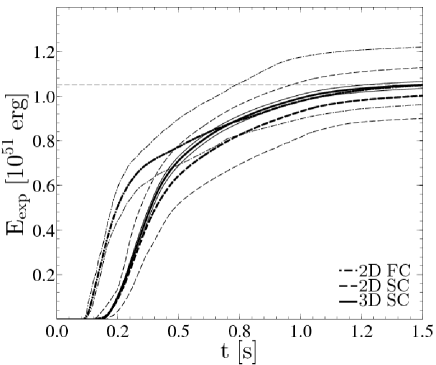
shows the explosion energy in models with both slow and fast contracting PNS cores. We show the mean explosion energy and the explosion energy envelope for 2D FC models (dash-dot), 2D SC models (dash), and 3D SC models (solid). In all cases, the explosion energy rises rapidly at the onset of explosion and approximately saturates by the final time. In the case of SC models, the explosion energy threshold is reached between 140 ms to 200 ms post-bounce depending on model realization. The two dimensional models tend to explode faster and reach their final energies later than the three dimensional models. The FC models explode significantly earlier, at approximately 110 ms on average. The short explosion times found in FC models, as compared to SC models, are not unexpected. This is because significantly greater neutrino luminosities, approximately by a factor of two, are required to energize the explosion in the presence of the deeper gravitational potential well in the FC models. Regardless of the contraction times of the PNS core, by the final time, s, and given the required explosion energetics and envelope mass, the average explosion energy in our models reaches about erg.
It is instructive to discuss our models in terms of the critical luminosity curve (Burrows & Goshy, 1993). We shall note that finding the curve was not the goal of our study, and therefore, we are not in a position to provide the exact relation. Our results only provide an upper limit on the critical neutrino luminosity for the (relatively small) range of accretion rates present in our models (see Table 2).
Figure 2
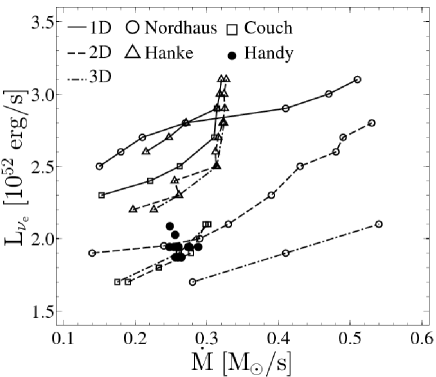
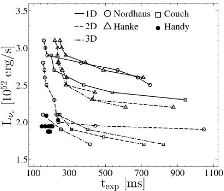
provides a comparison of our explosion models with the results of critical neutrino luminosity studies conducted by other groups. In the figure, the results of Nordhaus et al. (2010), Hanke et al. (2012), and Couch (2013) are shown with open circles, triangles, and squares, respectively, while our data are shown with solid circles; the model dimensionality is indicated with line style with solid, dashed, and dash-dotted lines connecting models obtained in 1D, 2D, and 3D, respectively. In the left panel, the neutrino luminosity is shown as a function of the accretion rate, which is measured by integrating the mass flux through the surface located just upstream of the shock at the onset of explosion.
This figure indicates that our choice to constrain the final explosion energy by observations required a relatively narrow range of neutrino luminosities, compared to other studies. We also find that the required neutrino luminosity systematically decreases as the dimensionality of the model increases. Neutrino luminosities found in our models only provide an upper limit for the critical luminosity for the mass accretion rates present in our simulations. Furthermore, explosion times found in our models are shorter than those of other groups for similar neutrino luminosities. The simplest explanation for this finding is that the neutrino heating is more efficient in our models. However, we cannot exclude the possibility that this observed, systematic difference is due to differences in the progenitors. Detailed investigation of possible differences between our findings and those of other groups is beyond the scope of the current work.
3.2. Neutron star recoil
Since we excise the neutron star from the grid, a special method has to be used to estimate its recoil velocity. To this end, we use the approach of Scheck et al. (2006), and exploit momentum conservation. In this method, the momentum of the neutron star balances the momentum of the surrounding envelope (total momentum on the mesh in our simulations). An additional correction can be applied to the neutron star recoil velocities by considering that the neutron star will continue accreting material beyond the final time in our simulations. We estimate the corrected velocity as
| (12) |
where is the recoil velocity obtained in our simulations at s, and is the approximate correction due to late time accretion onto the neutron star. To calculate the velocity correction, we assumed the rate of the recoil velocity change obtained by Scheck et al. (2006) in his B18 model series between the times s and s (see Figure 19 in Scheck et al., 2006),
| (13) |
Then the recoil velocity correction has been computed as
| (14) |
In the above formulae superscripts denote post-bounce explosion times, and the subscripts and denote the values from Scheck et al. (2006) and the current work, respectively.
Figure 3
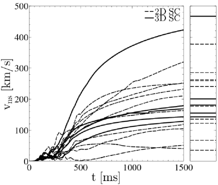
shows the evolution of recoil velocities in our models until the final time (left panel), and the estimated saturation velocities based on Equation 12 (right panel). Our results indicate relatively modest recoil velocities compared to Scheck et al. (2006). The approximate final recoil velocities are in the range between 100 km/s and 300 km/s, with the lowest and highest recoil velocities of 30 km/s and 475 km/s. These results are in qualitative agreement with the results reported by Scheck et al. (2006, Figure 20) and Wongwathanarat et al. (2013, B-series models in Table 2).
3.3. Gain region characteristics
In this section we report the results following the analysis of a quasi-steady state period in the pre-explosion epoch. If no such evolutionary stage is reached then the entire pre-explosion phase could be considered a transient phenomenon with little importance for the energetic core-collapse supernova explosions considered here. If the opposite is true however, we can adopt methods appropriate for analysis of quasi-steady state flows and apply them to analyze the dynamics of the gain region.
We identify the quasi-steady state period in the post-shock flow evolution by calculating the mass contained in the gain region, . Its time-dependence is shown in the left panel of Figure 4
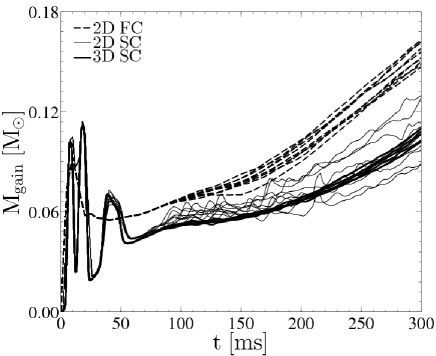
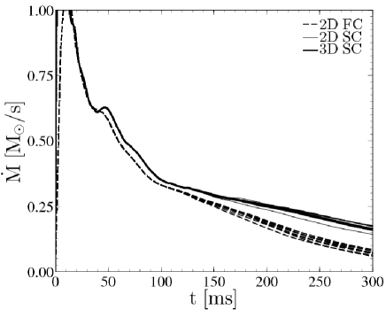
for our set of multidimensional models. As one can see, the mass in the gain region for the case of SC models (shown with solid lines) changes only slightly between ms and ms. A similar period of modest increase in the mass of the gain region can be found in the case of FC models (shown with dashed lines) for times between ms and ms. We note that in both cases, the moment when the mass in the gain region increases precedes the explosion times, which is consistent with a scenario in which the shock revival process occurs over an extended period of time in a quasi-steady state fashion. Also note the presence of strong oscillations in the gain region mass at early times in both families of models. Since, as we discuss below (Section 3.4), the shock radius is increasing steadily at these early times, the observed oscillations in the gain region mass are either due to density changes of the material entering the gain region or the changes in the position of the gain radius during these times. Those oscillations, however, have a transient character and do not play any role in the subsequent evolution of the system, and cease as soon as the flow in the gain region becomes multidimensional.
The mass accretion rate (shown in the right panel of Figure 4) as measured at the position of the shock front shows a rapid decline during the first 50 ms of the simulation time after which it steadily decreases at a progressively slower rate. The evolution of accretion rate does not differ significantly between SC and FC models. This is expected, as we consider only a single progenitor model. At later times when the quasi-steady state is reached, the accretion rates are between s-1 for SC models and between s-1 for FC models. The FC models are characterized by consistently lower accretion rates than the SC models for times later than 50 ms.
To better understand the dynamics in the gain region in the context of neutrino heating, we consider the advection timescale, ,
| (15) |
where is the mass in the gain region, and is the accretion rate. The advection time scale is the characteristic time a fluid parcel spends in the gain region. This quantity neglects multidimensional effects, which are known to be important in the process of shock revival. In the same context, we consider the heating efficiency, ,
| (16) |
where is the net neutrino energy deposition rate, and the integral in the above equation is taken over the gravitationally bound () material inside the gain region. The quantity in the denominator of the above equation is the heating timescale, i.e. the time it takes to heat a gravitationally bound fluid parcel so that it becomes unbound. The heating efficiency is a measure of the competition between the advection and heating processes. In particular, implies that the material in the gain region gains energy due to heating faster than it is removed by the advection process.
The time evolution of advective time for our sample of models is shown in Figure 5.
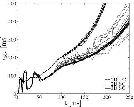
Since the advective time depends on the mass in the gain region, the oscillations in the advective time visible in Figure 5 prior to 50 ms are simply a reflection of the oscillations in the gain region mass (c.f. left panel in Figure 4). At later times, both SC and FC families (shown with solid and dashed lines in Figure 5) show qualitatively similar behavior. Again, this is expected due to a common progenitor model used in these calculations. Also, and as we discussed above, the variations between model realizations are due to differences that develop in multidimensional flow structure during the shock revival process.
We can compare the advective time to the length of the quasi-steady state phase of the evolution. For the SC models, we estimate the steady state lasts about 50 ms, while the advective time in this case is about 160 ms. In the case of FC models, we estimate the steady state lasts about 50 ms, but the advective time is somewhat shorter (about 100 ms). We conclude that in our models, on average, fluid parcels enter the gain region and reside in it during the entire process of shock revival. This conclusion is consistent with the history of individual fluid parcels (see Section 5.3 below).
The advective times found in our simulations are 3 to 10 times larger than those reported by Müller et al. (2012). We initially suspected that this significant difference in advective times might be due to general relativistic effects in the potential carefully accounted for by Müller et al. in their model. However, we believe the most probable explanation is the difference in the model energetics obtained in the two studies. This is because in the models of Müller et al. the shock resides during the shock revival phase for long times at much lower radii ( km) than in our models (– km). Therefore, provided the accretion rates are similar, the gain region has much lower mass in their models, resulting in correspondingly shorter advective times.
The evolution of heating efficiency is shown in Figure 6.
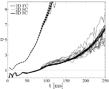
It is interesting to note a qualitative similarity between the SC and FC model families (shown with solid and dashed lines in the figure). For example, we note a period of modest increase in heating efficiency between ms and ms in FC models, and ms and ms in SC models. This increase in the heating efficiency is associated with the onset of convection prior to the quasi-steady state phase (see Section 4). At later times, after the quasi-steady state is established, the heating efficiency continues to steadily increase in the SC models while the increase in the heating efficiency is significantly greater in the FC models. Nevertheless, the heating efficiency continues to evolve in a qualitatively similar manner in both families of models. As we noted before, the similarities between SC and FC models can be easily explained by the fact that we consider only a single progenitor model in this work.
On the quantitative level, the heating efficiency in the FC models is greater than one from the beginning of the evolution. On the other hand, the heating becomes efficient in the SC models only after the quasi-steady state is established. We conclude that a strong, immediate neutrino heating is required in order to produce energetic explosions.
3.4. Shock evolution
The shock revival process can also be studied by analyzing the time evolution of the shock radius. In particular, prolonged periods of shock stagnation may indicate the onset of the standing accretion shock instability (SASI). Conversely, a steady increase in the shock radius may indicate that other processes (e.g. neutrino-driven convection) operate efficiently. Additionally, the unbinding of shocked matter is directly dependent on radius (through the gravitational potential), and large shock radii may aid in reaching the explosion threshold. Finally, hydrodynamic perturbations present at early times can be imprinted on the shock and affect the morphology of the supernova ejecta. To this end, in the following discussion we use the shock aspect ratio to quantify the explosion asymmetry.
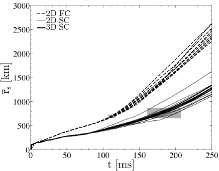
The evolution of the average shock radius, , in our models is shown in Figure 7 with solid and dashed lines for the SC and FC models, respectively. The shock radius increases steadily in both families of models, although the shock expansion is about 25% faster in the FC models. At the time when the early convection sets in, the shock expands to about 270 km in the FC models and about 200 km in the SC models. By the time the shock is revived, its average radius for different model realizations varies between 645 km and 855 km in the 2D SC models, and between 790 km and 810 km in the 3D SC models. We believe the greater variation in the average shock radius in the 2D models compared to 3D may hint at differences in the dynamics of the gain region between 2D and 3D. Moreover, 2D FC models display a similar amount of variation in the average shock position as 2D SC models. Also, in that case, the average shock position at the time of explosion varies between 640 km and 730 km. Overall, the average shock radius at the time of explosion is similar in SC and FC families. One should keep in mind, however, that the FC models explode, on average, twice faster than the SC models (c.f. Table 2).
The shock aspect ratio, , found in our models (see Figure 8)
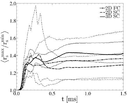
appears relatively modest compared to the shock asymmetry reported in other studies (Hanke et al., 2012; Müller et al., 2012). Although an extreme shock aspect ratio of was found in 2D SC simulations, the average aspect ratios are only 1.25 in 2D and 1.4 in 3D. This should be compared to the shock aspect ratios between and we estimated based on the data presented by Müller et al. (2012).
The most striking feature of the evolution of the shock aspect ratios in our models are strong asymmetries observed in the 2D SC models at early times. These asymmetries seem to rapidly decrease for times ms. In contrast, the shock aspect ratios in the 2D FC models appear to evolve more smoothly and the most deformed FC models seem to retain their asymmetric character as time progresses. Qualitatively, however, the degree to which the shock is deformed in 2D models is modest and on average is . In 3D models, the average degree of shock asymmetry at late times is somewhat greater (), and the variations between the individual 3D model realizations are less than %.
We speculate that the smooth evolution and persistent character of deformations found in the 2D FC models might be due to weaker convection which operates over a shorter period. Conversely, in 2D SC models convection has more time to organize the flow inside the gain region. Occasionally, the dominant mode develops in those models (cf. Figure 10(a)) and results in a strong asymmetry. In other 2D SC models, the higher order modes make the shock more spherical (cf. Figure 10(b)). The situation is similar in the case of 3D SC models, in which the post-shock region shows richer convective structure and evolves on a similar timescale as in 2D.
The evolution of shock radius also provides information that is helpful in the context of the standing accretion shock instability (SASI). Specifically, SASI manifests itself as low-order () oscillations of the shock radius (Foglizzo et al., 2006; Laming, 2007; Scheck et al., 2008; Foglizzo, 2009). Therefore, the first step in the SASI analysis of the shock revival is to decompose the shock radius in terms of spherical harmonics. The expansion coefficients are given by
| (17) |
where the spherical harmonic is normalized by a factor , and .
In order to enable direct comparison between the 2D () and 3D () cases, we consider a suitably normalized contribution of the -mode coefficients (Ott et al., 2013),
| (18) |
The evolution of and coefficients is shown in Figure 9.
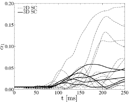
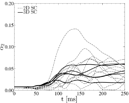
The larger values of the coefficients indicate that the 2D SC models, on average, exhibit stronger variability than their three-dimensional counterparts. However, we also observe a certain dichotomy among 2D SC models with one subgroup showing variability distinctly larger than the remaining set of models. 2D SC models also show relatively weak mode contributions. perturbations, while others rise to a moderate fraction of the average shock position. The 2D FC models (data not shown in Figure 9) show a similar degree of variability as the 2D SC models at all times.
Prior to explosion, the 2D models exhibit at most one or two weak oscillations. This is a quantitatively different behavior than found in the simulations of Müller et al. (2012), who reported strong, multiple cycles leading up to shock revival. In addition, the shock perturbations in our models are weak compared to those considered as evidence for SASI. Furthermore, we do not find qualitative differences between the 2D and 3D models, as we mentioned above. Note that most evidence for SASI presented in the literature is essentially restricted to 2D, non-exploding models.
In our SC models, the low order modes emerge at about ms, shortly before the quasi-steady state is established in the gain region. Visual inspection of the flow morphology during the quasi-steady state provides no evidence for large-scale “sloshing” motions in the gain region, considered a defining signature of SASI. We conclude it is unlikely the SASI plays any important role in the evolution of our models.
3.5. Morphology of the gain region
As soon as the neutrino-driven convection sets in and the related perturbations reach the shock, one faces a difficult problem of disentangling various physics processes participating in the shock revival, including fluid instabilities and neutrino-matter interactions. Analysis of the overall flow morphology is the first step in the process of understanding the explosion mechanism. It provides initial evidence for the physics of fluid flow participating in re-energizing the stalled shock (Herant et al., 1994). It also may provide evidence for the possible role of model parameters, such as assumed symmetries and discretization errors, e.g. near the symmetry axis (Scheck et al., 2006; Gawryszczak et al., 2010), on the flow dynamics. In this section we present the morphological evolution of our SC models in two and three dimensions. In particular, we are interested in identifying when the fluid flow instabilities imprint their structure on the just-formed inner core of the supernova ejecta.
Entropy pseudocolor maps of the gain region for two two-dimensional and two three-dimensional SC models at their respective explosion times are shown in Figure 10.
| \begin{overpic}[height=199.16928pt,viewport=115.43124pt 115.43124pt 988.69374pt 924.45374pt,clip]{fig10a.pdf} \put(82.0,78.0){\huge$\mathrm{\left(a\right)}$} \put(17.0,16.0){\large$\mathrm{M194J}$} \put(17.0,10.0){\large$\mathrm{t_{exp}=148\;ms}$} \put(-7.0,39.0){\large\rotatebox{90.0}{$\mathbf{r\;\left[km\right]}$}} \put(46.0,-7.0){\large{$\mathbf{z\;\left[km\right]}$}} \end{overpic} | \begin{overpic}[height=199.16928pt,viewport=115.43124pt 115.43124pt 988.69374pt 924.45374pt,clip]{fig10b.pdf} \put(82.0,78.0){\huge$\mathrm{\left(b\right)}$} \put(17.0,16.0){\large$\mathrm{M194C}$} \put(17.0,10.0){\large$\mathrm{t_{exp}=202\;ms}$} \put(-7.0,39.0){\large\rotatebox{90.0}{$\mathbf{r\;\left[km\right]}$}} \put(46.0,-7.0){\large{$\mathbf{z\;\left[km\right]}$}} \end{overpic} |
| \begin{overpic}[height=199.16928pt,viewport=115.43124pt 115.43124pt 988.69374pt 924.45374pt,clip]{fig10c.pdf} \put(82.0,78.0){\huge$\mathrm{\left(c\right)}$} \put(17.0,16.0){\large$\mathrm{M187A}$} \put(17.0,10.0){\large$\mathrm{t_{exp}=189\;ms}$} \put(-7.0,39.0){\large\rotatebox{90.0}{$\mathbf{y\;\left[km\right]}$}} \put(46.0,-7.0){\large{$\mathbf{x\;\left[km\right]}$}} \end{overpic} | \begin{overpic}[height=199.16928pt,viewport=115.43124pt 115.43124pt 988.69374pt 924.45374pt,clip]{fig10d.pdf} \put(82.0,78.0){\huge$\mathrm{\left(d\right)}$} \put(17.0,16.0){\large$\mathrm{M187B}$} \put(17.0,10.0){\large$\mathrm{t_{exp}=193\;ms}$} \put(-7.0,39.0){\large\rotatebox{90.0}{$\mathbf{y\;\left[km\right]}$}} \put(46.0,-7.0){\large{$\mathbf{x\;\left[km\right]}$}} \end{overpic} |
Prior to reaching the explosion threshold, the 2D SC models evolve to have either dipolar (, Figure 10(a)) or quadrupolar (, Figure 10(b)) ejecta morphology. These flow features emerge when strong downflows in the gain region are formed shortly after the onset of convection. Furthermore, our models indicate that these flow structures do not evolve once they set in and continue to persist after the explosion is launched, evolving in a self-similar fashion at later times (see below). Additionally, these downflows carry accreted material deep into the gain region close to the gain radius. This behavior does not seem to be as extreme in 3D SC models, because a comparable amount of accreted material is transported through many more downflows (see Figure 10(c) and (d)). The presence of many downflows in three-dimensions reflects the fact that the flow structure is inherently different in 2D and 3D. We quantify this behavior later in Section 4.
The entropy distribution in the 3D SC model M187A is shown in Figure 11 for select times.
| \begin{overpic}[width=128.0374pt,viewport=139.52124pt 105.39374pt 927.465pt 858.20624pt,clip]{fig11a.pdf} \put(80.0,80.0){\large$\mathrm{\left(a\right)}$} \put(15.0,10.0){\large$\mathrm{t=50\;ms}$} \put(-10.0,32.0){\rotatebox{90.0}{$\mathbf{y\;\left[10^{5}\;cm\right]}$}} \put(37.0,-7.0){{$\mathbf{x\;\left[10^{5}\;cm\right]}$}} \end{overpic} | \begin{overpic}[width=128.0374pt,viewport=139.52124pt 105.39374pt 927.465pt 858.20624pt,clip]{fig11b.pdf} \put(80.0,80.0){\large$\mathrm{\left(b\right)}$} \put(15.0,10.0){\large$\mathrm{t=100\;ms}$} \put(-10.0,32.0){\rotatebox{90.0}{$\mathbf{y\;\left[10^{5}\;cm\right]}$}} \put(37.0,-7.0){{$\mathbf{x\;\left[10^{5}\;cm\right]}$}} \end{overpic} | \begin{overpic}[width=128.0374pt,viewport=139.52124pt 105.39374pt 927.465pt 858.20624pt,clip]{fig11c.pdf} \put(80.0,80.0){\large$\mathrm{\left(c\right)}$} \put(15.0,10.0){\large$\mathrm{t=150\;ms}$} \put(-10.0,32.0){\rotatebox{90.0}{$\mathbf{y\;\left[10^{5}\;cm\right]}$}} \put(37.0,-7.0){{$\mathbf{x\;\left[10^{5}\;cm\right]}$}} \end{overpic} |
| \begin{overpic}[width=128.0374pt,viewport=139.52124pt 105.39374pt 927.465pt 858.20624pt,clip]{fig11d.pdf} \put(80.0,80.0){\large$\mathrm{\left(d\right)}$} \put(15.0,10.0){\large$\mathrm{t=189\;ms}$} \put(-10.0,32.0){\rotatebox{90.0}{$\mathbf{y\;\left[10^{6}\;cm\right]}$}} \put(37.0,-7.0){{$\mathbf{x\;\left[10^{6}\;cm\right]}$}} \end{overpic} | \begin{overpic}[width=128.0374pt,viewport=139.52124pt 105.39374pt 927.465pt 858.20624pt,clip]{fig11e.pdf} \put(80.0,80.0){\large$\mathrm{\left(e\right)}$} \put(15.0,10.0){\large$\mathrm{t=500\;ms}$} \put(-10.0,32.0){\rotatebox{90.0}{$\mathbf{y\;\left[10^{6}\;cm\right]}$}} \put(37.0,-7.0){{$\mathbf{x\;\left[10^{6}\;cm\right]}$}} \end{overpic} | \begin{overpic}[width=128.0374pt,viewport=139.52124pt 105.39374pt 927.465pt 858.20624pt,clip]{fig11f.pdf} \put(80.0,80.0){\large$\mathrm{\left(f\right)}$} \put(15.0,10.0){\large$\mathrm{t=1500\;ms}$} \put(-10.0,32.0){\rotatebox{90.0}{$\mathbf{y\;\left[10^{7}\;cm\right]}$}} \put(37.0,-7.0){{$\mathbf{x\;\left[10^{7}\;cm\right]}$}} \end{overpic} |
At early times, the flow evolves away from initially spherically symmetric accretion, with the first signs of convective instability emerging around ms (Figure 11(a)). At this time, the shock is not affected by convection. At intermediate times ( ms, Figure 11(b)), the initial convective plumes gradually merge into larger structures and begin deforming large segments of the shock front. As time progresses, the process of bubble merging continues (Figure 11(c)) and the shock eventually is launched around ms (Figure 11(d)).
The large-scale morphology of the post-shock region appears essentially frozen after the explosion commences. For example, three ejecta plumes seen in the southern hemisphere (Figure 11(d)), can still be easily identified more than 300 ms later (Figure 11(e)). However, during the same period the convective bubbles in the northern hemisphere show significant evolution and appear to merge into a single structure. This morphology persists until the end of the simulation and the central region becomes filled with the neutrino-driven wind (Figure 11(f)).
4. Convection
Our analysis of the explosion process presented above revealed that the explosion is preceded by a relatively short (compared to other studies) quasi-steady state inside the gain region (Section 3.3) during which the shock only slowly expands and SASI does not seem to a major role (Section 3.4). We also found that the heating becomes efficient shortly before the quasi-steady state is established (Section 3.3).
There exists a large body of evidence from numerical simulations of core-collapse supernova explosions indicating that multidimensionality, and specifically the presence of convection, decreases the requirements for the neutrino luminosity produced by the contracting core of the proto-neutron star (Janka & Mueller, 1996; Nordhaus et al., 2010; Hanke et al., 2012; Couch, 2013). In this section we focus on characterization and quantification of the effects of neutrino-driven convection during the quasi-steady state of the gain region. We introduce and apply novel methods dedicated to investigating this aspect of the supernova explosion process.
4.1. Minimum resolution requirements
We perform a series of three-dimensional simulations in order to assess the dependence of model physics operating inside the gain region on numerical resolution. In particular, we are interested in finding conditions required to suppress neutrino-driven convection on large scales. If indeed convection is a critical component driving the explosion, one could expect that by suppressing convection (by whatever means) the explosion would not occur, even in models with neutrino luminosities that in other situations are sufficiently large enough to revive the shock. This expectation is strongly supported by numerous calculations which show that, for example, much higher luminosities are required to produce an explosion in one-dimension than in multidimensions (see, e.g., Janka & Mueller (1996), Section 3.3, and Figure 2 for discussion and compilation of relevant recent results).
In our series of 3D simulations, we keep the radial resolution fixed while the angular resolution is gradually decreasing by a factor of 2 between the models, from 3∘ (our base resolution) down to 24∘. In addition, we compute a 2∘ resolution model. For each model, we recorded the explosion times and explosion energies at ms. The basic characteristics of models obtained in this series is given in Table 3.
| Angular | ||
|---|---|---|
| Resolution | (ms) | ( erg) |
| 2∘ | 183 | 0.114 |
| 3∘ | 183 | 0.107 |
| 6∘ | 175 | 0.106 |
| 12∘ | 198 | 0.077 |
| 24∘ | 216 | 0.028 |
The inspection of data shown in the table reveals that the explosion times and the explosion energies change little as long as the angular resolution is not worse than 6∘. For coarser angular meshes, we observe a significant increase in the explosion times and decrease in the explosion energies. No explosions were found at resolutions coarser than 24∘.
It is conceivable that the observed changes in global model characteristics should be correlated with changes in the flow structure inside the gain region. Figure 12
| \begin{overpic}[width=199.16928pt,viewport=133.49875pt 113.42374pt 978.65623pt 917.42749pt,clip]{fig12a.pdf} \put(82.0,82.0){\huge$\mathrm{\left(a\right)}$} \put(17.0,12.0){\huge$\mathrm{3^{\circ}}$} \put(-9.0,40.0){\large\rotatebox{90.0}{$\mathbf{y\;\left[km\right]}$}} \put(45.0,-7.0){\large{$\mathbf{x\;\left[km\right]}$}} \end{overpic} | \begin{overpic}[width=199.16928pt,viewport=133.49875pt 113.42374pt 978.65623pt 917.42749pt,clip]{fig12b.pdf} \put(82.0,82.0){\huge$\mathrm{\left(b\right)}$} \put(17.0,12.0){\huge$\mathrm{6^{\circ}}$} \put(-9.0,40.0){\large\rotatebox{90.0}{$\mathbf{y\;\left[km\right]}$}} \put(45.0,-7.0){\large{$\mathbf{x\;\left[km\right]}$}} \end{overpic} |
| \begin{overpic}[width=199.16928pt,viewport=133.49875pt 113.42374pt 978.65623pt 917.42749pt,clip]{fig12c.pdf} \put(82.0,82.0){\huge$\mathrm{\left(c\right)}$} \put(17.0,12.0){\huge$\mathrm{12^{\circ}}$} \put(-9.0,40.0){\large\rotatebox{90.0}{$\mathbf{y\;\left[km\right]}$}} \put(45.0,-7.0){\large{$\mathbf{x\;\left[km\right]}$}} \end{overpic} | \begin{overpic}[width=199.16928pt,viewport=133.49875pt 113.42374pt 978.65623pt 917.42749pt,clip]{fig12d.pdf} \put(82.0,82.0){\huge$\mathrm{\left(d\right)}$} \put(17.0,12.0){\huge$\mathrm{24^{\circ}}$} \put(-9.0,40.0){\large\rotatebox{90.0}{$\mathbf{y\;\left[km\right]}$}} \put(45.0,-7.0){\large{$\mathbf{x\;\left[km\right]}$}} \end{overpic} |
shows the entropy maps in a subset of the models used in this resolution study. One can easily note profound structural changes in the morphology of the gain region as the angular model resolution decreases. Large- and small-scale convective bubbles can clearly be seen in the 3∘ resolution model (panel (a)). There are significantly fewer small, convective bubbles present in the 6∘ model (panel (b)). In those two models the overall shock radius appears comparable. In contrast, no well-defined, small-scale bubbles can be identified in the 12∘ or 24∘ models (shown in panels (c) and (d), respectively). In addition, the shock radius is visibly smaller in the 24∘ model.
We interpret the observed dependence of energetics and explosion timing on angular resolution described above as follows. Consider that the hydrodynamic solver used in our simulations is the PPM scheme (Colella & Woodward, 1984). PPM is nominally third order (and practically second order) accurate in space, and uses piece-wise parabolic interpolation to describe profiles of the hydrodynamic state. Therefore, the minimal number of mesh resolution elements required to resolve a convective bubble is about 3 mesh cells. In our 12∘ and 24∘ resolution models there are only 13 and 7 cells in angle, respectively. This implies our hydrodynamic solver can only represent between 2 to 4 large-scale structures in those models. The number of those structures does not represent the actual number of bubbles, as some mesh cells are also required to describe the flow structure between the bubbles. This explains the lack of bubbles on smaller scales and the overall degraded appearance of the neutrino-driven convection in these cases.
We demonstrated through this resolution study that the neutrino-driven convection is a critical component of the explosion mechanism in our models. Specifically, we have shown that one can turn an energetic, multidimensional model into a failed multidimensional model simply by degrading its angular resolution. Therefore, to correctly capture the efficiency of the convective engine one needs to resolve its basic components. This picture is also consistent with the analysis of Herant et al. (1994), who argued that, independent of dimensionality, large scales will play the dominant role in convection. Furthermore, it is important to resolve not only structures on the largest scales, but also the structures on ∘ are important. We conclude with the somewhat obvious statement that capturing the relevant physics of the problem requires adequate numerical resolution. It is conceivable that the next generation of ccSNe models with much higher resolution will begin uncovering new physics effects that cannot be observed in the current generation of models due to their insufficient quality.
4.2. Dynamics
One of the quantities of interest in the context of dynamics of convection is the amount of mass contained inside rising, convective bubbles. To characterize that quantity, we introduce the upflow mass fraction,
| (19) |
where the integration is performed over the gain region, and takes into account only the fluid elements (grid zones) with positive radial velocity. Thus, the upflow mass fraction characterizes the mass inside the gain that is moved away from the proto-neutron star toward the shock. The evolution of the upflow mass fraction in our models is shown in Figure 13.
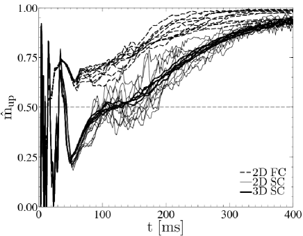
As one can see, the initial behavior of the upflowing mass is characterized by a transient period until ms. Soon after that, the amount of upflowing mass begins to steadily increase. It levels off during the quasi-steady state phase lasting approximately between – ms for SC models (shown with solid lines in Figure 13) and – ms for FC models (shown with dashed lines in Figure 13), and rises again after the shock is launched. Interestingly, the net mass flux inside the gain region is close to zero in the SC models (the horizontal dashed line at ), while upflows dominate in the FC models. This can be qualitatively understood considering that energetic explosions in the case of fast contracting proto-neutron star cores require much higher neutrino luminosities in order to unbind a sufficiently large amount of material inside the gain region. This indicates that perhaps convection plays a smaller role in FC models compared to SC models. Also note that the amount of upflowing mass begins to differ between various model realizations shortly before the quasi-steady state is established. Those variations are greater in 2D than in 3D (for SC models). Ultimately, after the explosion is in progress, the amount of upflowing mass steadily increases and eventually levels off, signifying the fact of the overall expansion of the material inside the gain region.
It is interesting to note that the observed behavior in the upflowing mass fraction, in particular its steady increase after the transient period, is closely correlated with the evolution of the heating efficiency (cf. Figure 6). For example, the heating efficiency becomes greater than 1 in the SC models before the amount of upflowing material becomes comparable to the amount of accreted material. In addition, the heating efficiency is always greater than 1 in the case of FC models, where upflows dominate at all times.
Figure 14 shows the time evolution of the fluctuations in the upflowing mass in the gain
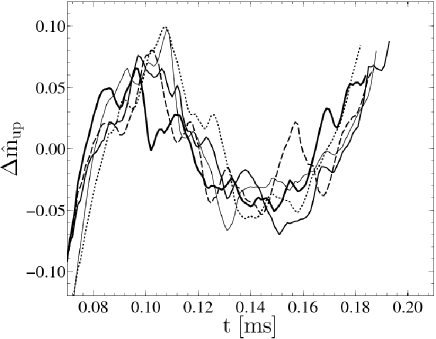
region in the 3D SC models as a function of time around the quasi-steady phase. It is interesting to note that the increase of the outflowing mass in these models is non-monotonic. One can identify several short ( ms) episodes during which the amount of mass in upflows fluctuates. These fluctuations have an amplitude of several percent. Given that the typical number of convective bubbles, and therefore also the number of downflows, in those models during the quasi-steady state phase is about to (see Section 4.3), it is conceivable that perhaps individual downflows are responsible for the observed fluctuations.
4.3. Characterization of convective structures
Having in mind the continuing debate regarding the role of dimensionality in numerical models of ccSNe explosions, we seek information about the dependence of large-scale structure of convection inside the gain region on model dimension. As the first step in our analysis, we wish to measure the net radial momentum over a fraction of the gain region,
| (20) |
where is the angle-dependent midpoint between the shock and gain radii ( and , respectively), is the angle-dependent gain region width, and is a fractional offset between and which controls the extent of the gain region included in the integration. We use the above equation to project average properties of the radial flow and distinguish between regions dominated by either upflows () or downflows (). Recall that our models are essentially free of possible SASI contributions, and therefore this method should be applicable to any convective flows.
Apart from the situation when the shock and gain radius are constant, the radial extent of the integration bounds in the above equation will vary with angle. In this way, we avoid possible ambiguities that may arise near those two regions, and make the results of this method insensitive to flow asymmetries naturally developing especially along the shock front. In the above equation we heuristically set so that our results are based on the data over the middle 20% of the gain region (at a given angle).
We use the maps produced with the help of the above equation to create connected clusters of upflow-like and downflow-like sections. We identify the upflow-dominated clusters with the rising convective bubbles. The solid angle spanned by each bubble is simply computed by integrating the area of the upflow-dominated cluster.
The time evolution of the total solid angle occupied by bubbles for the SC models is shown in Figure 15 (with data for 2D and 3D models shown by dashed and solid lines, respectively).
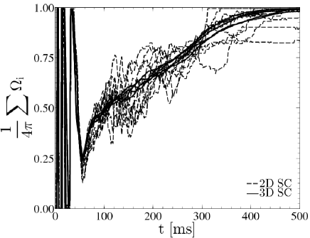
Prior to the onset of convection ( ms), the whole gain region oscillates radially. As convective structures begin to emerge, the solid angle occupied by bubbles starts to increase. This process starts to slow down at the beginning of the quasi-steady state phase ( ms). However, and unlike in the case of other diagnostics we have discussed above, the evolution of the solid angle occupied by bubbles does not provide any clear signature of the explosion time. Rather, the growth continues at a similar pace until about 150 ms after the explosion commences. It starts to level off soon after that time, and by 400 ms after bounce the whole gain region is filled-in with upflowing material.
Apart from large-amplitude oscillations, the evolution of the solid angle occupied by bubbles in 2D SC models is qualitatively similar to that seen in 3D, with the average value similar between the models. However, in a few 2D cases persistent downflows develop (see also Section 3.5). For these models the solid angle occupied by bubbles does not reach by the end of the period we analyzed here. Note that our diagnostics can be use to identify situations when strong accretion onto the proto-neutron star continues at late times.
Figure 16
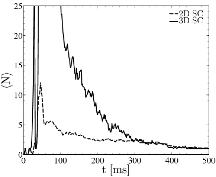
shows the time evolution of the number of bubbles inside the gain region averaged separately for 2D and 3D SC models (shown with dashed and solid lines, respectively). Initially, our method identifies only a single bubble or finds no bubble during the initial transient ( ms), in agreement with the radial oscillations of the gain region during that period as we discussed earlier. Soon after convection sets in, the number of distinct upflows sharply increases, reaching in 2D and in 3D. (Note, for the purpose of presentation we have limited the scale in Figure 16 to 25.) Given that at those early times the solid angle occupied by bubbles is small, we conclude that the bubbles are initially small and grow in angular extent over time. By the time of the explosion, the bubbles are roughly 4 times smaller in 3D than in 2D.
Recall that in 2D the bubbles are truly tori rather than quasi-spherical plumes. We recognize this may have certain implications for the bubble dynamics (see, e.g., Kifonidis et al., 2003; Hammer et al., 2010; Couch, 2013). Furthermore, the observed evolution of bubble sizes from small to large (see also Herant et al., 1994) offers an interesting parallel between the evolution of the structure of neutrino-driven convection (and perhaps convection in general), and that of bubble merger observed in a multi-mode Rayleigh-Taylor instability (see, e.g., Alon et al., 1994; Miles, 2004). The study of the process of merging convective bubbles is beyond the scope of the present work.
The growth of convective bubbles after ms coincides with time at which the heating efficiency starts to increase (cf. Figure 6) and accumulation of mass in the gain region (cf. Figure 4). We believe this indicates that early, small-scale convection begins to interact with the incoming accretion flow, resulting in rather rapid increase in the gain region mass. Subsequently, the advection time scale also increases. We believe this provides evidence for the direct dependence of the heating efficiency on the intensity of convection.
4.4. Convective energy transport
In our discussion of convective energy transport, we adopt the approach originally introduced for the analysis of stellar convection by Hurlburt et al. (1986). In this approach, the individual components of the energy transport equation, Equation 3, are averaged over lateral directions. Then, one computes radial distributions of deviations away from the lateral averages, . In the discussion here, we use the notation of Mocák et al. (2009). We define the convective flux, , kinetic flux, , buoyant work, , and expansion work, , as follows:
| (21) |
| (22) |
| (23) |
| (24) |
where the integrals are taken over the suitable solid angle (in our models with the excised ∘ cone around the symmetry axis this amounts to % of the full solid angle). These terms describe the total energy transported per unit time through a surface of a sphere of radius .
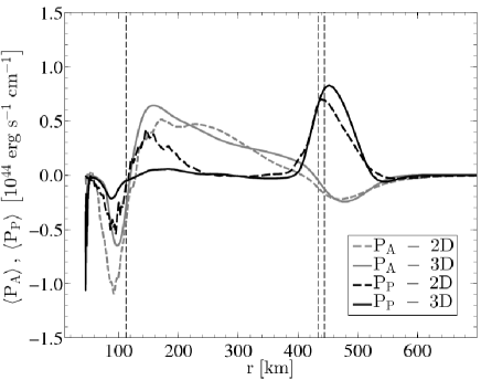
Figure 17
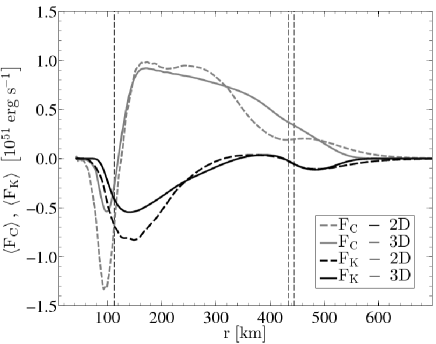
shows the time averages of convective and kinetic energy fluxes (left panel) and the buoyant and expansion work terms (right panel) for the SC models. The main characteristics of the energy transport follow from the direction of the energy transport and the relative contributions of individual terms. We begin our analysis at the gain radius located at km in both 2D and 3D models (marked with the solid, vertical line). There, the convective flux is initially negative but rapidly increases and reaches the maximum at % of the radial extent of the gain region. Further out, the convective flux gradually decreases and ultimately ceases well upstream of the shock. On the other hand, the kinetic energy flux is negative below the gain radius and remains negative through most of the gain region. The observed run of the convective flux provides clear evidence for convective transport in which material heated near the gain radius buoyantly rises toward the shock.
The relation between buoyancy and convection also manifests itself through the buoyant work, (shown with gray lines in the right panel of Figure 17). The work done by buoyancy becomes positive starting at the gain radius, indicative of buoyancy driving the convection upwards. It first rapidly increases through the bottom layers of the gain region, and reaches its maximum at % of the gain region extent. Further out, the work done by buoyancy gradually decreases and eventually vanishes as expected at the shock, where the flow becomes, on average, spherically symmetric.
As we noted, the buoyant work is positive throughout the gain region. This can be caused by either overdense material sinking or underdense material rising. Since the work due to buoyancy is negative below the gain region, therefore the opposite scenario with either overdense, cold material is rising or underdense, hot material is sinking. Since we do not observe sinking of the underdense, hot material in that region, we conclude that the negative work due to buoyancy indicates the presence of rising overdense and cold matter. In our models, this rising, overdense material originates from the downflows that are turned around by the pressure gradient. This process is known as buoyant braking (Brummell et al., 2002).
The most conspicuous difference between 2D and 3D lies in the distribution and value of the expansion work source term, (shown with solid lines in the right panel of Figure 17). When integrated over time and space, this term represents the work of fluid elements. Below the gain radius this term is negative, indicative of the work done in the process of compressing the fluid. It changes sign across the gain radius, and remains positive through the lower one-third of the gain region. This indicates that the fluid is expanding in that region. We quantify the amount of work due to expansion by integrating Equation 24 over the portion of domain between km and km, where the expansion work source term is significant and differs most between 2D and 3D. Assuming a characteristic timescale of ms, we estimate the (kinetic) energy change due to work to be erg and erg in 2D and 3D, respectively, or about a few percent of the explosion energy.
We believe the difference in the work, as we described above, reflects the fact that the structural integrity of upflows and downflows in 2D is much greater than in 3D. The structural integrity of flow features depends on the surface-to-volume ratio. For a given volume, 2D structures have less surface area than their 3D counterparts. Thus, flow structures in 2D are less susceptible to (surface) perturbations. We alluded to this property in our discussion of morphological differences between 2D and 3D simulations in Section 3.5. Consequently, in 3D, the downflows do not penetrate as deep, which can be clearly seen in the left panel of Figure 17, which shows that both the kinetic fluxes are negative and of comparable magnitude in both 2D and 3D around km. However, as one moves into deeper layers the kinetic flux much more rapidly decreases in 2D than in 3D, and vanishes in the layers closer to the proto-neutron star surface. The convective fluxes in 2D and 3D behave in a qualitatively similar way, although they are positive and equal closer to the gain radius, at km. From there inward, the convective flux decreases at a significantly greater rate across the gain radius and ceases closer to the proto-neutron star surface in 2D than in 3D. Furthermore, the greater structural integrity of upflows and their coherent nature in 2D makes the expansion process dramatically more efficient than in 3D. This is evidenced by much greater work done by expansion above the gain radius, as we discussed earlier.
As one can see in the right panel of Figure 17, the buoyant and expansion terms are both negative below the gain region. This is because below the gain region the system is no longer energy conserving due to intense neutrino heating. This situation is different, however, across the shock front. There, both terms are of different sign, which is consistent with the fact that the neutrino heating is weak and the energy is approximately conserved in that region.
Finally, we would like to note an interesting possibility that the difference in efficiency of the convective engine between 2D and 3D might be another consequence of the difference in surface-to-volume ratio between those models. This is because in 3D the surface area of the interface between hot and cold material where the mixing, and thus also heat exchange, takes place is relatively larger. Quantifying this possibly important effect is, however, beyond the scope of this paper.
5. Turbulence
Motivated by the recent discussion of the possible role of turbulence in the process of shock revival (Murphy & Meakin, 2011; Hanke et al., 2012), we present spectra of the kinetic energy in a lateral direction and turbulent Reynolds stresses characteristic of the gain region for our SC models. In particular, we will determine if the kinetic energy spectra are consistent with model dimensionality, and discuss the qualitative differences in the Reynolds stresses found between 2D and 3D.
5.1. Spectra
We investigate the spectral properties of turbulence by considering the spherical harmonic decomposition of Equation 17 with , where is the polar component of the velocity vector. Our choice of this particular velocity component hinges on the assumption that the flow is isotropic in the lateral directions, which is supported by our analysis of the Reynolds stresses presented below in Section 5.2.
To ensure that the energy contained in the spherical harmonic modes adequately represents the lateral kinetic energy, we include the factor (Endeve et al., 2012). Following Hanke et al. (2012), we define the lateral kinetic energy spectrum, , as
| (25) |
where the integral is taken over the solid angle included in our simulations. In order to account for spatial and temporal variations of the lateral kinetic energy spectrum, we average the spectrum over a shell of thickness km centered at the midpoint of the gain region ( km). In addition, in our analysis the spectra are averaged over snapshots from the time interval between ms and ms (soon after the quasi-steady state phase). In passing we note that there exists other choices of physical quantities for the analysis of turbulence, for example density fluctuations (Borriello et al., 2013), which are more suited for the analysis of neutrino-matter interactions rather than fluid flow dynamics.
Figure 18
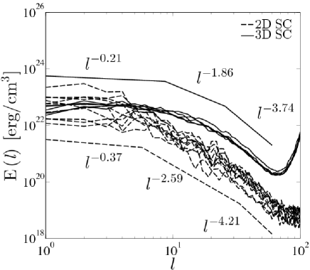
shows the lateral kinetic energy spectra for our SC models with 2D and 3D models shown with dashed and solid lines, respectively, averaged over time and space as described above. We find that one can identify three distinct spectral regions in the lateral kinetic energy spectrum. The first region occupies large scales ( a few), the intermediate region extends up to several 10s, and the third region extends toward still smaller scales (). This resembles spectra routinely found in turbulence studies, with the highest end of our spectrum closely resembling the region found in numerical simulations. It is customary to characterize those regions by a piecewise-linear combination of powerlaws, . In particular, it is expected that in the intermediate regime, in which the energy is transported from large to small scale (and possibly also in the opposite direction in 2D situations), a cascade develops with the power law exponent, , chiefly dependent on the particular characteristics of the system.
To quantify the shape of the power spectra found in our simulations, we fit power law functions inside each region. We found that the power law exponent that best characterizes the shape of the spectrum at large scales is (in 3D) to (in 2D). On the other extreme, the spectrum steepens around with . At still smaller scales (), the spectrum abruptly changes its shape presumably due to numerical dissipation.
Of the greatest interest from the point of view of turbulence are energy-transporting intermediate scales (a few ). We find that in this region the power spectra in 2D simulations are significantly steeper () than in 3D (). This is qualitatively consistent with the results of turbulence studies in 2D. We also note that the power law exponent found in 3D is not too dissimilar from that of the classic Kolmogorov spectrum (; Monin & I’Aglom (1971)).
On a final note, the Reynolds number estimated for our models is quite small (s s, see Appendix A), characteristic of perturbed laminar flow rather than turbulence. We caution one should be careful with drawing any conclusions regarding the turbulent character of such underresolved numerical models (Murphy & Burrows, 2008; Murphy & Meakin, 2011; Hanke et al., 2012). Furthermore, our models do not account for additional physics effects that may play an important role at the base of the convective region, such as neutrino viscosity (see discussion in Section 3.1 of Fryer & Young (2007)). These effects may actually reduce the physical Reynolds number down to , which is comparable to the numerical Reynolds number found in our simulations. Studying such effects, however, is beyond the scope of the present work.
5.2. Turbulent Reynolds stresses
Figure 19
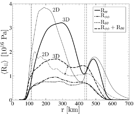
shows the time- and model realization-averaged turbulent Reynolds stress components for the SC models. The data shown in the figure were generated as follows. First, the tensor components were computed for individual model realizations using
| (26) |
where denotes the averaging operation over solid angle, is the perturbation away from the background of the -th component of velocity, and is the background density. After averaging over the solid angle, the stress components were then averaged over the period between ms and ms. In the final step, we used these averages to compute the model-averaged values of turbulent Reynolds stresses.
In 3D, the radial (shown with the thick solid line in Figure 19) and lateral stress components (shown with thick dash-dotted and dotted lines; their sum is shown with the thick dashed line), increase from the inner boundary and across the gain radius (marked with a vertical, dashed line at km). The radial component reaches the maximum around km, roughly in the middle of the gain region, while the overall contribution of lateral stresses peaks slightly deeper at km. The radial stress is about a factor of greater than the sum of lateral stresses. Farther out, the stresses decrease and reach approximately similar magnitude just below the shock. In the figure, the three dashed, vertical lines located between 400 km and 600 km mark the innermost, average, and outermost shock radii. The stresses show a mild increase across the region occupied by the shock and eventually vanish upstream of the shock inside the accretion flow. The sum of lateral stresses exceeds the radial stress by % in a relatively narrow region behind the shock (at km). Before we begin discussing the qualitative and quantitative between the average turbulent Reynolds stresses in 2D and 3D, we note that the radial dependence of stresses in 2D (shown with thin solid and dash-dotted lines for the radial and lateral stresses, respectively, in Figure 19) is quite similar to that in 3D. Moreover, flow appears roughly isotropic below the gain radius, with radial and lateral stresses in equipartition.
We note that the stresses in 2D are much larger in the region near the gain radius than in 3D. This can be understood by recalling that the convection is most vigorous in that region in our two-dimensional models (see Section 4.4). Farther out, the dominant, buoyantly-generated radial stresses undergo redistribution in lateral directions (see, e.g., Murphy & Meakin (2011)). This process of redistribution of the radial stress is expected to be isotropic in the lateral directions, as observed in our 3D simulations (thick dash-dotted and dotted lines in Figure 19). By volume-integrating the radial averages of the stress components inside the gain region, we find that in both 2D and 3D the integrated radial stress is larger by about % than the lateral stresses. Furthermore, the integrated turbulent stresses are greater by about % in 3D than in 2D. The latter result may appear at first surprising, judging by the run of turbulent stresses shown in Figure 19. However it is important to recognize that the curves shown in the figure represent angular averages rather than volume-integrated contributions. Therefore, even though the stresses are greater in 2D than in 3D near the gain radius, the larger stresses in 3D in the upper layers of the gain region result in their overall greater volume-integrated value.
The fact that the volume-integrated turbulent stresses are greater in 3D than in 2D is consistent with the surface-to-volume difference between 2D and 3D simulations (the argument we made in Section 4.4). In this scenario, 3D structures are more susceptible to perturbations and the flow becomes disorganized over larger regions (in our case, a greater fraction of the radial extent of the gain region). Specifically, full-width at half-maximum measure of the radial stress distribution is % greater in 3D than in 2D. (The corresponding volume factor is still larger due to the 3D distribution being centered at a higher radius.) Finally, we note that the process of redistribution of the radial stress is appears more gradual in 3D than in 2D (compare the two curves connected with the double arrow in Figure 19). In fact, this may only be a misimpression. Note that the contribution of lateral stresses in 2D differs qualitatively from that in 3D only in the lower half of the gain region. We find preliminary evidence that this may be due to the difference in the work done by expansion in that region, where the expansion work source term is large in 2D, while it is nearly zero in 3D (see Figure 17). We speculate that the expansion increases the velocity fluctuations and thus contributes to the increase of the turbulent stresses.
5.3. Lagrangian analysis of the explosion mechanism
We believe that potentially important insights into the core-collapse supernova explosion mechanism can be gained through analyzing the history of fluid parcels as they enter the gain region and participate in the revival of the shock. Our motivation partially follows from the realization that the amount of evidence provided by the Eulerian analysis appears insufficient to disentangle and clearly identify the role various physics plays in the explosion process. To this end, we seeded our simulations with a large number of tracer particles from the beginning of the simulations. Recall from Section 2 than in our models, each tracer particle represents a fluid element with a mass of in two-dimensions and in three-dimensions.
5.3.1 Residence times in the gain region
In our analysis we assume a particle resides inside the gain region if its position is between the shock radius and the gain radius (both of which are angle- and time-dependent). We define the residency time, , as the total time a tracer particle spends in the gain region. Thus, the maximum residency time of any particle never exceeds the model time elapsed since the beginning of the simulation. We construct a distribution of particle residency times by binning the residency times with a resolution of ms.
Figure 20
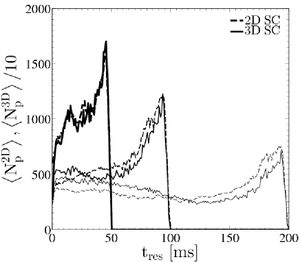
shows the model realization-averaged distributions of particle numbers for our SC models at ms, 100 ms, and 200 ms, as a function of particle residency time. In the figure, the data for 2D and 3D models are shown with dashed and solid lines, respectively. The total number of particles in the gain region are approximately , , and in 2D and , , and in 3D, for progressively later evolutionary times. We note that particles occupying bins near should be interpreted as material that has been just accreted (entered the gain region), while the farther to the right the particle bin is the earlier it entered the gain region.
There is little difference in distributions of particle numbers between the 2D and 3D models (shown with thick dashed and solid lines, respectively, in Figure 20) for particles that enter the gain region prior to the onset of convection. This is expected, given that at those early times the shock is nearly spherically symmetric and the post-shock flow is essentially radial. These initial distributions are expected to evolve due to both accretion of new material (particles passing through the shock), and loss of particles already residing in the gain region through the gain radius and their settling onto the proto-neutron star. Therefore, one may expect certain differences in the distributions of particle numbers at later times. First, notice that the number of particles with maximum residency times is always smaller in 3D than in 2D, except at the early time ( ms). This means that a portion of particles with the longest residency times that are accreted through the gain radius is larger in 3D than in 2D. Second, this trend reverts at , and at ms there are more particles with short residency times present in 3D than in 2D. One possible explanation for this behavior might be a systematic differences in accretion rates and shock radii between 2D and 3D, but we found no evidence to support this possibility (cf. Section 3.3).
Additional information about the origin and evolution of particle number distributions can be obtained by examining the spatial dependence of particle residency times. These distributions reveal that, in 3D, there exists a population of particles with low residency times located near the gain radius. The systematic differences between particle number distributions in 2D and 3D can therefore be explained by particles leaving and reentering the gain region across the gain radius in 3D. This leads to the apparent deficit of particles with long residency times and causes excess of particles with low residency times in this case. We quantified the magnitude of this effect by examining the contours of cumulative particle numbers at a given residency time. We found that between % and % of particles located near the gain radius participate in this process. This estimate is consistent with the difference between the particle number distributions seen in Figure 20. The above effect signifies a difference in the flow dynamics near the gain radius between 2D and 3D. In particular, we believe this behavior is due to a larger amount of mass (by –%) involved in convection at the bottom of the gain region, where the convection is driven, and may be the reason for the greater efficiency of convection in 3D (see Section 5.3.3 for discussion).
5.3.2 Thermodynamic evolution of the shocked material
One quantity of particular interest in the context of the ccSNe explosion mechanism is the boost to the internal energy of the material residing in the gain region provided by neutrino heating. This process can be analyzed by considering the increase in the internal energy of shocked fluid parcels (represented in our study by tracer particles) as a function of the particle residency time.
Figure 21
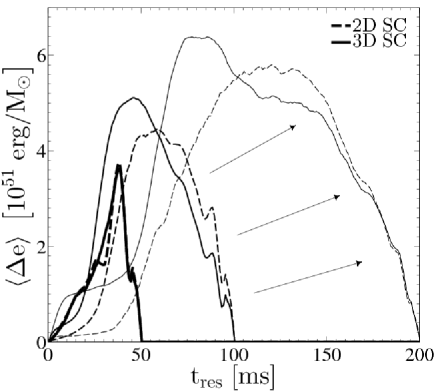
shows the model realization-averaged internal energy gain per unit mass, , as a function of particle residency time for the 2D and 3D SC models (shown with dashed and solid lines, respectively). We define the internal energy gain of a tracer particle as the difference between the particle internal energy at the evolutionary time shown and its internal energy when it enters the gain region. We find that at early times ( ms) there is essentially no difference in the way particles gain energy in 2D and 3D (thick dashed and solid lines). At later times, we begin to observe modest at first ( ms) changes with the newly accreted material progressively gaining energy faster in 3D than in 2D (the solid, medium thick line representing 3D data lies always to the left of the dashed, medium thick line representing the 2D data).
In addition to the apparent asymmetry in the 3D distribution at late times, we also find qualitatively new unique features, in particular at ms. First, we identify a region with almost constant increase in the energy gain for particles that entered the gain region between ms and ms. During this time, and as we discussed earlier in Section 5.3.1, the gain radius shrinks faster in 3D than in 2D. This allows the particles residing close to the gain radius to gain comparatively more energy in 3D. This process is responsible for the observed shape of the internal energy gain distribution for residency times between ms and ms. Second, there is a pronounced hump visible in Figure 21 which broadly occupies a ms time interval for particles that entered the gain region shortly after the vigorous convection developed. This is marked by a rapid increase in the 3D energy gain curve taken at ms (thin solid line) at ms. We believe this signifies the increase in the thermodynamic efficiency of the convective engine in 3D. Third, there is a smaller hump for a population of particles that entered the gain region shortly before ( ms) the shock was launched.
Finally, we would like to point out that the similarity in the shapes of the 3D distributions at late times is quite striking. The arrows in the figure connect specific features in the energy gain distributions that are well preserved in 3D between ms and ms. This indicates that the particles which entered the post-shock region during the first ms of the simulation gained internal energy at a similar rate during the process of shock revival.
5.3.3 Unbinding of the shocked material
The explosion process necessarily requires gravitationally unbinding a substantial fraction of the collapsing core. Alas, very little information about this process can be found in the literature, perhaps with the exception of discussions of global quantities such as the explosion energy. However, armed with the tracer particles we are now in a position to investigate this process in more detail. In particular, the results discussed in the previous section indicate that profound differences in the heating efficiency exist between 2D and 3D models. Although we are able to identify populations of particles responsible for those differences, our focus was more on the interplay between the advection and neutrino heating of the shocked material. In the following discussion of the process of gravitational unbinding of the shocked, stellar core we also take into account the flow dynamics inside the gain region.
Figure 22
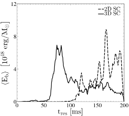
shows the model realization-average of the positive part of the specific gravitational binding energy, , as a function of residency time for 2D and 3D families of models at ms (marked by dashed and solid lines, respectively). The data indicates dramatic differences in the energetics of fluid elements in the gain region between 2D and 3D. In 2D, the unbound portion of the gain region is almost exclusively made of material that entered the gain region during the first ms of the evolution. However, in 3D one can identify two different populations of particles. The first 3D population consists of particles that entered the gain during the first ms. Although this is the same material that is responsible for the explosion in 2D, in 3D this material is substantially less energetic. A careful examination of the data shown in Figure 22 reveals that, indeed, around the explosion time the explosion energies in 2D are greater than in 3D. This is consistent with the 2D models exploding, on average, faster than 3D models. Also, as discussed in the previous section, the particles that enter the gain region early on gain energy more efficiently in 2D than in 3D. It is only at later times when the particles in 3D show a dramatic increase in their internal energies.
In the scenario presented above, the explosion is launched in 2D early on by a relatively stronger central neutrino source. In 3D, however, the more efficient convective engine is able to launch the shock at neutrino luminosities lower by %. (Recall that we found evidence for up to % more mass participating in convection across the gain radius in 3D, as discussed in Section 5.3.1). By integrating the particle energies, we found that in 3D the same amount of positive binding energy is carried by particles that entered the gain region during the first ms of evolution as by those which entered the gain region during the following ms. Thus, the process of unbinding material in the gain region appears more gradual in three-dimensions, with significant energy gain during the quasi-steady phase.
The cause of the observed differences between energetics in 2D and 3D ccSNe simulations, and so the question how the efficiency of the convective engine depends on dimensionality, remains unknown at this time. However, we believe the Lagrangian approach to analyzing the evolution of the gain region offers significant advantages over Eulerian statistics for investigating the efficiency of convection. This will problem will be the subject of a forthcoming publication.
6. Summary & future work
We have presented an analysis of two- and three-dimensional models of early core-collapse supernova development in the collapsing core of a progenitor. In our study, the simulations start at shock bounce, continue through the onset of neutrino-driven convection, quasi-steady state of the gain region, and early post-revival shock expansion until the energy of the explosion had approximately saturated at 1.5 seconds. Our models were tuned to match the estimated explosion energetics of SN 1987A by careful selection of the parameterized neutrino luminosity. We considered the cases of slow and fast contraction rates of the proto-neutron star to reflect on uncertainty in the nuclear equation of state. We introduced and applied new diagnostic methods for the explosion process, morphology and structure of convection, and energetics of material inside the gain region.
Our conclusions are formulated based on a large database of explosion models. This computationally expensive approach is necessary since the core-collapse supernova problem involves highly nonlinear, strongly coupled physics which results in the extreme sensitivity of realistic computational models to perturbations. Therefore, conclusions of core-collapse supernova studies can only be understood in a statistical sense. Moreover, such ensemble-based conclusions are potentially affected by resolution effects, especially in three-dimensions, due to the high computational cost of individual model realizations.
The main findings of our work can be summarized as follows:
-
•
We found that the same explosion energy can be obtained in three-dimensions with less energy than in two-dimensions. This trend also holds between two-dimensions and one-dimension. This result is in agreement with some previous studies.
-
•
The stochastic character of the explosion process results in non-uniqueness of the relation between neutrino luminosity and explosion energy. In particular, in the process of tuning the neutrino luminosities, we were able to obtain equally energetic 3D models with the neutrino luminosities differing by as much as %.
-
•
Dimensionality also contributes to the non-uniqueness of the above relation. In particular, equally energetic explosions can be obtained in 3D using neutrino luminosities smaller by % than in 2D. This implies the efficiency of the convective engine is greater by that amount in 3D.
-
•
We proposed that the observed dependence of the efficiency of the convective engine on the model dimensionality might be a consequence of the difference in the surface-to-volume ratio of flow structures between 2D and 3D. In this scenario, the greater efficiency of the convective engine in 3D is simply due to a larger surface-to-volume ratio in that case, which helps the process of heat exchange between hot and cold flow structures. Quantifying this possibly important effect is, however, beyond the scope of this paper.
-
•
We note that the relations between neutrino luminosities, accretion rates, and explosion times show, in our models, less variation with the model dimensionality than in other studies (see Figure 2). We believe this is purely due to the fact that the objective of our study was to obtain models with similar energetics, rather than to determine the threshold neutrino luminosity required for the explosion.
-
•
We found no evidence for the standing accretion shock instability (SASI) in our models. Our results showed no persistent, oscillatory or mode behavior, considered to be a trademark of SASI. The absence of SASI in our models is consistent with short advective times through the gain region. Instead, the explosions are boosted in multidimensions by strong, neutrino- driven convection. At the same time, we would like to stress that SASI cannot be excluded as an important, or even decisive, physics mechanism for different parameters of collapsing core (e.g., progenitor structure, equation of state, etc.).
-
•
We found that the shock front shows a rather modest degree of asymmetry in our models, . We found tentative evidence between the large-scale structure of convection and the shock asymmetry. In particular, the shock is less deformed in the case when convection has a richer structure (higher-order modes are present).
-
•
We found the neutron star recoil velocities reaching up to km/s, with typical values between km/s and km/s. These results are in good agreement with the previous studies (e.g. Scheck et al., 2006).
-
•
We introduced and applied new metrics to diagnose the dynamics and structure of the gain region. In particular, we studied the characteristics of the upflowing material (which we identified as the buoyant, convective bubbles) and the solid angle it occupies. Using these measures, we found that the structure of the gain region on large scales and its evolution did not significantly differ between 2D and 3D. However, for the fast contracting models, we found that the mass inside upflows always exceeded % of the total gain region, hinting at prompt-like explosions. This situation is qualitatively different in the case of the slow contracting models, where a prolonged period of quasi-steady state in the gain region can be clearly recognized. It appears that during that phase the mass in the upflows fluctuates around the slowly increasing mean value with amplitude of several percent, and on a timescale of 10 ms. We speculate that individual downflows are responsible for the observed fluctuations.
-
•
Our method of identifying the convective bubbles allowed us to study the statistical properties of the bubble distributions. We found that the solid angle occupied by bubbles is initially small and progressively increases with time (see Figure 15). This indicates that the bubbles are small at first and steadily grow as the evolution progresses. The process appears to bear some similarity to the bubble merging process observed in multi-mode Rayleigh-Taylor instabilities. Furthermore, we find a good correlation between the solid angle occupied by rising material and the upflowing mass. This highlights the convection takes place inside the whole gain region, from the gain radius all the way up to the shock.
-
•
The development and evolution of convection inside the gain region can also be studied by considering the temporal evolution of the number of bubbles. We found that their number rapidly increased at ms (see Figure 16), indicating the onset of convection. After the convection set in, the number of bubbles progressively decreased with time. We used the information about the number of bubbles combined with the solid angle they occupy, and estimated that the convective bubbles are, on average, about 4 times smaller in 3D than in 2D at the time of the explosion.
-
•
We used the decomposition of the total energy flux to understand the energy transport in the gain region. We found that the work done by expansion and compression in that region differs between 2D and 3D, and we proposed that this is due to the greater structural integrity of flow structures in 2D.
-
•
The analysis of the components of the total energy flux also provided evidence that the region near the gain radius was not in thermal equilibrium at the beginning of the quasi-steady phase. We found evidence for strong cooling below and strong heating above the gain radius. Furthermore, we found that the buoyant work was positive throughout the gain region in our models, in accordance with the neutrino-driven convection scenario.
-
•
We demonstrated that, for the same neutrino luminosities that produce energetic explosions in well-resolved models, the explosion energies dramatically decrease once the angular mesh resolution decreases below 6∘. This implies there exists a minimal mesh resolution required for the central engine to efficiently operate. This is expected. This also implies that the neutrino-driven convection is the key ingredient of the explosion mechanism in the energetic models considered here. We cannot exclude the possibility that more physics (e.g. turbulence) may emerge at still higher resolutions (i.e. less than about ) to power the explosion more efficiently than convection.
-
•
We found that the the structure of turbulent energy spectra are steeper in our 2D models () than in our 3D models (). These results should be taken with caution given the low resolution of our models and an estimated Reynolds number on the order of .
-
•
Analysis of the turbulent Reynolds stresses revealed that the post-shock flow is anisotropic in the radial direction due to buoyant driving. At the same time, we found the flow in the gain region is isotropic in the lateral directions.
-
•
Using a Lagrangian representation of the gain region, we found substantial differences in the energetics of the shocked fluid elements between 2D and 3D. We identified material near the base of the gain region that experiences stronger heating during the period when the gain radius shrinks. We also found that material accreted during the phase when the convection is fully developed undergoes especially strong heating in 3D.
-
•
We found significant differences in the evolution of residency times and binding energies of fluid elements inside the gain region between 2D and 3D. In 3D, more mass is involved in the process of driving convection in the region around the gain radius. At the same time, the same amount of positive binding energy is carried by material that entered the gain region during the first ms of evolution as by those which entered the gain region during the following ms. However, in 2D, a smaller portion of the gain region mass participates in driving convection, and practically all of the positive binding energy is carried by material that entered the gain region during the first ms.
Several possible directions for future research emerge from the current work. It remains unclear why the convective engine is more efficient in three-dimensions. Although we were able to quantify the effect, we did not provide a clear explanation for its origin. We obtained only rudimentary information about the properties of turbulence in our largely underresolved and dominated by numerical viscosity models. It is clear that to gain meaningful insight into the role of turbulence in the process of core-collapse supernova explosion a new generation of far better-resolved models exploiting more efficient computational approaches is required. Also, one would like to evolve those models until the neutron star recoil velocities saturate. Finally, our current model does not include nuclear burning, and therefore we are unable to discuss the nucleosynthetic yields and the compositional structure of our models. The above issues will be the subject of a forthcoming publication.
References
- Alon et al. (1994) Alon, U., Hecht, J., Mukamel, D., & Shvarts, D. 1994, Physical Review Letters, 72, 2867
- Arnett (1987) Arnett, W. D. 1987, ApJ, 319, 136
- Blinnikov (1999) Blinnikov, S. I. 1999, Astronomy Letters, 25, 359
- Blondin & Mezzacappa (2007) Blondin, J. M., & Mezzacappa, A. 2007, Nature, 445, 58
- Blondin et al. (2003) Blondin, J. M., Mezzacappa, A., & DeMarino, C. 2003, ApJ, 584, 971
- Borriello et al. (2013) Borriello, E., Chakraborty, S., Janka, H.-T., Lisi, E., & Mirizzi, A. 2013, ArXiv e-prints
- Bruenn (1993) Bruenn, S. W. 1993, in Nuclear Physics in the Universe, ed. M. W. Guidry & M. R. Strayer (Bristol: IOP), 31–50
- Bruenn et al. (2013) Bruenn, S. W., Mezzacappa, A., Hix, W. R., et al. 2013, ApJ, 767, L6
- Brummell et al. (2002) Brummell, N. H., Clune, T. L., & Toomre, J. 2002, ApJ, 570, 825
- Burrows (2013) Burrows, A. 2013, Reviews of Modern Physics, 85, 245
- Burrows & Goshy (1993) Burrows, A., & Goshy, J. 1993, ApJ, 416, L75
- Chugai (1988) Chugai, N. N. 1988, Pis’ma Astronomicheskii Zhurnal, 14, 1079
- Colella & Glaz (1985) Colella, P., & Glaz, H. M. 1985, J. Comput. Phys., 59, 264
- Colella & Woodward (1984) Colella, P., & Woodward, P. R. 1984, J. Comput. Phys., 54, 174
- Couch (2013) Couch, S. M. 2013, ApJ, 775, 35
- Dolence et al. (2013) Dolence, J. C., Burrows, A., Murphy, J. W., & Nordhaus, J. 2013, ApJ, 765, 110
- Einfeldt (1988) Einfeldt, B. 1988, SIAM J. Num. Anal., 25, 294
- Endeve et al. (2012) Endeve, E., Cardall, C. Y., Budiardja, R. D., et al. 2012, ApJ, 751, 26
- Foglizzo (2009) Foglizzo, T. 2009, ApJ, 694, 820
- Foglizzo et al. (2006) Foglizzo, T., Scheck, L., & Janka, H.-T. 2006, ApJ, 652, 1436
- Frisch (1995) Frisch, U. 1995, Turbulence: the legacy of A.N. Kolmogorov
- Fryer & Warren (2002) Fryer, C. L., & Warren, M. S. 2002, ApJ, 574, L65
- Fryer & Young (2007) Fryer, C. L., & Young, P. A. 2007, ApJ, 659, 1438
- Gawryszczak et al. (2010) Gawryszczak, A., Guzman, J., Plewa, T., & Kifonidis, K. 2010, A&A, 521, A38
- Hammer et al. (2010) Hammer, N. J., Janka, H.-T., & Müller, E. 2010, ApJ, 714, 1371
- Hanke et al. (2012) Hanke, F., Marek, A., Müller, B., & Janka, H.-T. 2012, ApJ, 755, 138
- Herant et al. (1994) Herant, M., Benz, W., Hix, W. R., Fryer, C. L., & Colgate, S. A. 1994, ApJ, 435, 339
- Hurlburt et al. (1986) Hurlburt, N. E., Toomre, J., & Massaguer, J. M. 1986, ApJ, 311, 563
- Imshennik & Popov (1992) Imshennik, V. S., & Popov, D. V. 1992, AZh, 69, 497
- Janka et al. (2003) Janka, H.-T., Buras, R., Kifonidis, K., Plewa, T., & Rampp, M. 2003, in From Twilight to Highlight: The Physics of Supernovae, ed. W. Hillebrandt & B. Leibundgut, 39
- Janka et al. (2012) Janka, H.-T., Hanke, F., Hüdepohl, L., et al. 2012, Progress of Theoretical and Experimental Physics, 2012, 010000
- Janka & Mueller (1996) Janka, H.-T., & Mueller, E. 1996, A&A, 306, 167
- Kifonidis et al. (2003) Kifonidis, K., Plewa, T., Janka, H.-T., & Müller, E. 2003, A&A, 408, 621
- Kifonidis et al. (2006) Kifonidis, K., Plewa, T., Scheck, L., Janka, H.-T., & Müller, E. 2006, A&A, 453, 661
- Laming (2007) Laming, J. M. 2007, ApJ, 659, 1449
- Lattimer & Swesty (1991) Lattimer, J. M., & Swesty, D. F. 1991, Nuclear Physics A, 535, 331
- Marek et al. (2006) Marek, A., Dimmelmeier, H., Janka, H.-T., Müller, E., & Buras, R. 2006, A&A, 445, 273
- Mezzacappa et al. (1998) Mezzacappa, A., Calder, A. C., Bruenn, S. W., et al. 1998, ApJ, 495, 911
- Miles (2004) Miles, A. R. 2004, Physics of Plasmas, 11, 5140
- Mocák et al. (2009) Mocák, M., Müller, E., Weiss, A., & Kifonidis, K. 2009, A&A, 501, 659
- Monin & I’Aglom (1971) Monin, A. S., & I’Aglom, A. M. 1971, Statistical fluid mechanics; mechanics of turbulence
- Müller et al. (2012) Müller, B., Janka, H.-T., & Heger, A. 2012, ApJ, 761, 72
- Murphy & Burrows (2008) Murphy, J. W., & Burrows, A. 2008, ApJ, 688, 1159
- Murphy & Meakin (2011) Murphy, J. W., & Meakin, C. 2011, ApJ, 742, 74
- Nordhaus et al. (2010) Nordhaus, J., Burrows, A., Almgren, A., & Bell, J. 2010, ApJ, 720, 694
- Ohnishi et al. (2006) Ohnishi, N., Kotake, K., & Yamada, S. 2006, ApJ, 641, 1018
- Ott et al. (2013) Ott, C. D., Abdikamalov, E., Mösta, P., et al. 2013, ApJ, 768, 115
- Pumo & Zampieri (2011) Pumo, M. L., & Zampieri, L. 2011, ApJ, 741, 41
- Rampp & Janka (2002) Rampp, M., & Janka, H.-T. 2002, A&A, 396, 361
- Scheck (2007) Scheck, L. 2007, Phd thesis, Technische Universität München
- Scheck et al. (2008) Scheck, L., Janka, H.-T., Foglizzo, T., & Kifonidis, K. 2008, A&A, 477, 931
- Scheck et al. (2006) Scheck, L., Kifonidis, K., Janka, H.-T., & Müller, E. 2006, A&A, 457, 963
- Shigeyama & Nomoto (1990) Shigeyama, T., & Nomoto, K. 1990, ApJ, 360, 242
- Strang (1968) Strang, G. 1968, SIAM J. Numer. Anal., 5, 506
- Takiwaki et al. (2013) Takiwaki, T., Kotake, K., & Suwa, Y. 2013, ArXiv e-prints
- Utrobin (1993) Utrobin, V. 1993, A&A, 270, 249
- Utrobin (2004) Utrobin, V. P. 2004, Astronomy Letters, 30, 293
- Utrobin (2005) —. 2005, Astronomy Letters, 31, 806
- Utrobin & Chugai (2005) Utrobin, V. P., & Chugai, N. N. 2005, A&A, 441, 271
- Wongwathanarat et al. (2013) Wongwathanarat, A., Janka, H.-T., & Müller, E. 2013, A&A, 552, A126
- Woosley (1988) Woosley, S. E. 1988, ApJ, 330, 218
Appendix A Estimating numerical viscosity and Reynolds number
In order to estimate the numerical viscosity and the numerical Reynolds number, we use the information provided by the Lagrangian tracer particles. Consequently, in our approach the velocity field is represented at discrete points by tracer particles. We define the longitudinal Eulerian velocity structure function of order- as
| (A1) |
where is the particle position, is the particle velocity, is the separation between particles, and is the particle displacement unit vector. The averaging operator, , is applied over a given at a specific model time.
Kolmogorov’s turbulence theory (Monin & I’Aglom, 1971; Frisch, 1995), assuming negligible intermittence, states that for , the structure function, , is related to the average specific turbulent dissipation, , via
| (A2) |
where is a constant on the order of 1. This result allows one to estimate the turbulent dissipation (physical + numerical) present in a numerical simulation. Within the same framework, the local, specific turbulent dissipation is related to the average strain rate as
| (A3) |
where is the kinematic viscosity and is the strain rate tensor.
In order to estimate the numerical Reynolds number in our models, we assume that the local turbulent dissipation is representative of the average dissipation rate, . This allows us to compute the kinematic viscosity as
| (A4) |
Using as our characteristic length scale and approximating the characteristic velocity in the field by , we estimate the Reynolds number as a function of separation distance via
| (A5) |
Figure 23
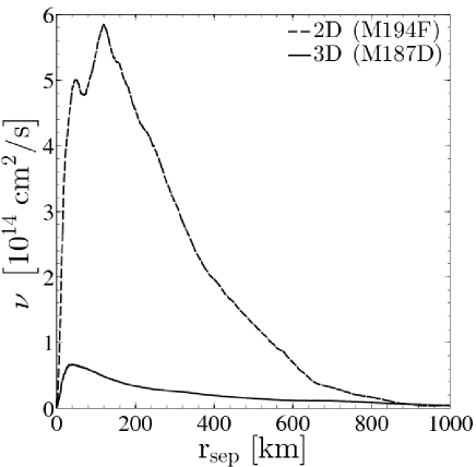
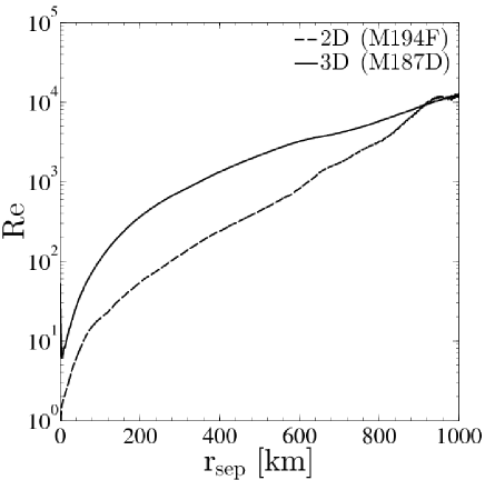
shows the numerical kinematic viscosity and numerical Reynolds number estimates for the 2D SC model M194J and the 3D SC model M187D at ms as a function of particle separation distance. We find numerical viscosities on the order of cm2s-1 for the 2D model and cm2s-1 for the 3D model. At this time in the model evolution, the average shock radius is about 500 km, providing an upper limit on structure size. On that scale, the numerical Reynolds number is in 2D and in 3D. However, as one can see, the numerical viscosity, and so the numerical Reynolds number, vary with scale. Therefore, our models cannot be represented by a single numerical Reynolds number. Consequently, and given relatively low values of the numerical Reynolds number present in our simulations, we tend to characterize the fluid flow inside the gain region of our models as perturbed laminar, rather than turbulent.
Finally, we would like to remark that given the anisotropy of the flow field obtained in our simulations (chiefly due to large-scale convection), the assumption that the average dissipation rate can be represented by the local dissipation rate may not hold true in all regions in our models. However, we believe that the obtained estimates still provide valuable insights into the nature of our simulations. In particular, given the low estimated numerical Reynolds numbers, conclusions regarding the role of turbulence in the core-collapse supernova explosions should be considered, at most, tentative. Since turbulence was not a particular focus of this study, we are not in a position to estimate the resolution required to capture these effects.