Generic framework for anisotropic flow analyses with multi-particle azimuthal correlations

Ante Bilandzic Niels Bohr Institute, Blegdamsvej 17, 2100 Copenhagen, Denmark    Christian Holm Christensen Niels Bohr Institute, Blegdamsvej 17, 2100 Copenhagen, Denmark    Kristjan Gulbrandsen Niels Bohr Institute, Blegdamsvej 17, 2100 Copenhagen, Denmark    Alexander Hansen Niels Bohr Institute, Blegdamsvej 17, 2100 Copenhagen, Denmark    You Zhou Nikhef, Science Park 105, 1098 XG Amsterdam, The Netherlands Utrecht University, P.O. Box 80000, 3508 TA Utrecht, The Netherlands
Abstract

We present a new generic framework which enables exact and fast evaluation of all multi-particle azimuthal correlations. The framework can be readily used along with a correction framework for systematic biases in anisotropic flow analyses due to various detector inefficiencies. A new recursive algorithm has been developed for higher order correlators for the cases where their direct implementation is not feasible. We propose and discuss new azimuthal observables for anisotropic flow analyses which can be measured for the first time with our new framework. The effect of finite detector granularity on multi-particle correlations is quantified and discussed in detail. We point out the existence of a systematic bias in traditional differential flow analyses which stems solely from the applied selection criteria on particles used in the analyses, and is also present in the ideal case when only flow correlations are present. Finally, we extend the applicability of our generic framework to the case of differential multi-particle correlations.

pacs:
25.75.Ld, 25.75.Gz, 05.70.Fh

I Introduction

In relativistic heavy-ion collisions the azimuthal anisotropy of the produced particles as a function of transverse momentum has emerged as the most renowned observable to study the collective properties of nuclear matter Ollitrault:1992bk . Due to the collision geometry in non-central heavy-ion collisions, the initial volume containing the interacting nuclear matter is anisotropic in coordinate space. Of particular interest is the scenario in which the produced nuclear matter managed to thermalize in this anisotropic volume, causing its initial anisotropy from the coordinate space to be transfered via mutual interactions into the resulting and observable anisotropy in momentum space. We refer to this phenomenon in this work as collective anisotropic flow, or just simply as flow. Clearly, collective anisotropic flow is a direct probe of the degree of thermalization of the produced matter, and correspondingly an indirect probe of its transport properties (e.g. viscosity).

Whatever its underlying cause is, the resulting anisotropic distribution in momentum space can always be expanded into Fourier series Voloshin:1994mz :

f(φ)=12π[1+2n=1vncos[n(φΨn)]].𝑓𝜑12𝜋delimited-[]12superscriptsubscript𝑛1subscript𝑣𝑛𝑛𝜑subscriptΨ𝑛f(\varphi)=\frac{1}{2\pi}\left[1+2\sum_{n=1}^{\infty}v_{n}\cos[n(\varphi-\Psi_{n})]\right]\,. (1)

The first few coefficients (harmonics) in the above series have by now been thoroughly studied by experimentalists as well as theorists: The first coefficient v1subscript𝑣1v_{1}, is usually referred to as directed flow, the second coefficient, v2subscript𝑣2v_{2}, is referred to as elliptic flow, the third coefficient, v3subscript𝑣3v_{3} is referred to as triangular flow, etc. ΨnsubscriptΨ𝑛\Psi_{n} denotes the symmetry plane of the harmonic vnsubscript𝑣𝑛v_{n} (in general different harmonics will have different symmetry planes). φ𝜑\varphi denotes the azimuthal angles of the produced particles. For the case of an idealized initial geometry in heavy-ion collisions, all symmetry planes coincide and are equal to the reaction plane of the collision (a plane spanned by the impact parameter and the beam axis). Given the above Fourier series expansion, one can show, using just the orthogonality properties of trigonometric functions, that

vn=cos[n(φΨn)],subscript𝑣𝑛delimited-⟨⟩𝑛𝜑subscriptΨ𝑛v_{n}=\left<\cos[n(\varphi\!-\!\Psi_{n})]\right>\,, (2)

where angular brackets denote an average over all particles in an event. Due to only mathematical steps involved in its derivation, we stress that Eq. (2) per se has no physical meaning. In particular, Eq. (2) can give rise to non-vanishing flow harmonics vnsubscript𝑣𝑛v_{n} irrespectively of whether the azimuthal anisotropy in the momentum distribution has its origin in collective anisotropic flow or in some other completely unrelated physical process which can also yield event-by-event anisotropies (e.g. mini-jets). We now attempt to attach a more rigorous treatment to the concept of “collectivity” by discussing which tools and observables we can utilize experimentally in order to disentangle it from processes which generally involve only a small subset of the produced particles, generally termed “nonflow”.

In order to make a statement on whether the harmonics vnsubscript𝑣𝑛v_{n} in Eq. (1) are dominated by contributions from collective anisotropic flow or by some other processes which are non-collective in nature, we can use correlation techniques involving two or more particles. In this paper our main focus will be on the latter, to which we refer to as multi-particle correlation techniques. When only collective anisotropic flow is present, all produced particles are independently emitted, and are correlated only to some common reference planes. This physical observation translates into the following mathematical statement:

f(φ1,,φn)=fφ1(φ1)fφn(φn).𝑓subscript𝜑1subscript𝜑𝑛subscript𝑓subscript𝜑1subscript𝜑1subscript𝑓subscript𝜑𝑛subscript𝜑𝑛f(\varphi_{1},\ldots,\varphi_{n})=f_{\varphi_{1}}(\varphi_{1})\cdots f_{\varphi_{n}}(\varphi_{n})\,. (3)

The left-hand side of Eq. (3) is a joint multi-variate probability density function (p.d.f.) of n𝑛n observables φ1,,φnsubscript𝜑1subscript𝜑𝑛\varphi_{1},\ldots,\varphi_{n}. The right-hand side of Eq. (3) is the product of the normalized marginalized p.d.f, fϕi(ϕi)subscript𝑓subscriptitalic-ϕ𝑖subscriptitalic-ϕ𝑖f_{\phi_{i}}(\phi_{i}), where 1in1𝑖𝑛1\leq i\leq n, which are the same Danielewicz:1983we and are given by Eq. (1). Therefore, when all particles are emitted independently, as is the case for collective anisotropic flow, the joint p.d.f. for any number of particles will factorize as in Eq. (3). Based on this reasoning, one can build up, in principle, infinitely many independent azimuthal observables sensitive to various combinations of flow harmonic moments and corresponding symmetry planes by adding more and more particles to the observables. When flow harmonics fluctuate event-by-event, different underlying p.d.f.’s of flow fluctuations will result in different values of flow harmonic moments and corresponding symmetry planes. This illustrates our main point: In order to determine the underlying p.d.f. of flow fluctuations, one is necessarily led towards multi-particle correlation techniques. We will elaborate on this point in detail and generalize it further in the main part of the paper. For completeness, we now present the historical overview of the utilization of multi-particle correlation techniques in anisotropic flow analyses, together with all of the technical limitations and issues inherit to them, which this paper overcomes.

Multi-particle correlation techniques in anisotropic flow analyses have been used for more than three decades. In the theoretical studies of global event shapes Danielewicz:1983we and in the subsequent study presented in Ollitrault:1992bk , the joint multi-variate p.d.f. of M𝑀M particles for an event with multiplicity M𝑀M was utilized in flow analyses for the first time. On the other hand, the very first experimental attempt to go beyond two-particle azimuthal correlations Wang:1991qh date back to Bevalac work published in Jiang:1992bw . In that paper, a quantitative description of collectivity was attempted by generalizing the observable for two-particle correlations, namely the smaller angle between the transverse momenta of two produced particles, into the geometric mean of n(n>2)𝑛𝑛2n\ (n>2) azimuthal separations within the n𝑛n-particle multiplet. However, it was realized immediately that the net contribution of low-order few-particle correlations is cumulative if one increases the number of particles in such multiplets, which triggered the demand for more sophisticated techniques that would instead suppress systematically such contributions for increasingly large multiplets Jiang:1992bw .

This was pursued further in a series of papers on multi-particle correlations and cumulants by Borghini et al (for a summary of the mathematical and statistical properties of cumulants we refer the reader to Kubo:1962 ). In the first paper of the series Borghini:2000sa , Borghini et al defined cumulants in the context of flow analyses in terms of the moments of the distribution of the Q𝑄Q-vector amplitude Ollitrault:1992bk ; Barrette:1994xr ; Voloshin:1994mz . As a landmark of their approach, the authors have introduced a formalism of generating functions accompanied with interpolation methods in the complex plane as the simplest and fastest way to calculate cumulants from experimental data. The formalism of generating functions is particularly robust against biases stemming from non-uniform detector acceptance, which is frequently the dominant systematic bias in anisotropic flow analyses. However, there were some serious drawbacks, which were recognized and discussed already by the authors in the original paper. Most notably, both two- and multi-particle cumulants were plagued by trivial and non-negligible contributions from autocorrelations, which caused an interference between the various harmonics. This led the authors to propose an improved version of the generating function in Borghini:2001vi , which by design generated cumulants free from autocorrelations. In essence, the way cumulants were defined conceptually has changed between the two papers: In Borghini:2001vi cumulants were defined directly in terms of multi-particle azimuthal correlations, which are free from autocorrelations by definition, while in Borghini:2000sa cumulants were defined in terms of the moments of the distribution of the Q𝑄Q-vector amplitude, which by definition have contributions from autocorrelations. Both methods to calculate cumulants were capable of estimating reference and differential flow. Further improvement, still relying on the formalism of generating functions, came with the Lee-Yang zero (LYZ) method Bhalerao:2003xf ; Bhalerao:2003yq , which isolates the genuine multi-particle estimate for flow harmonics, corresponding to the asymptotic behavior of the cumulant series. The formalism of generating functions, however, has its own built-in systematic biases. Most importantly, the proposed interpolating methods in the complex plane to calculate cumulants are not numerically stable for all values of flow harmonics and multiplicity (“parameter r0subscript𝑟0r_{0} has to be tuned”); in addition, one never exactly recovers the cumulants as they are defined (“the series expansion of the generating functions has to be terminated manually at a certain order, in order to close the coupled system of equations for the cumulants”); finally, the formalism as presented in these papers is limited to the cases where all harmonics in multi-particle correlators coincide. A notable alternative cumulant approach in terms of implementation was used in Adler:2002pu , which, at the expense of reducing statistics, removed autocorrelations by explicitly constructing multiple subevents from the original event.

These limitations were removed partially with Q𝑄Q-cumulants (QC) published recently in Bilandzic:2010jr , which do not rely on the formalism of generating functions, but instead utilize Voloshin’s original idea of expressing multi-particle azimuthal correlations analytically in terms of Q𝑄Q-vectors evaluated (in general) in different harmonics. Q𝑄Q-cumulants, however, are very tedious to calculate analytically, and such calculations were accomplished only for a rather limited subset of multi-particle azimuthal correlations which have been most frequently used in anisotropic flow analyses to date.

The present paper surpasses completely all technical limitations of these previous publications and provides a generic framework allowing all multi-particle azimuthal correlations to be evaluated analytically, with a fast single pass over the data, free from autocorrelations by definition, and corrected for systematic biases due to various detector inefficiencies (e.g. non-uniform azimuthal acceptance, pTsubscript𝑝Tp_{\rm T}-dependent reconstruction efficiency, finite detector granularity, etc.). With this framework, a plethora of new multi-particle azimuthal observables are now accessible experimentally. In this paper we propose and discuss some new concrete examples (so-called standard candles). We have paid special attention to the development of algorithms, which can be used to calculate recursively higher-order multi-particle azimuthal correlators in terms of lower-order ones, for the cases when their standalone generic formulae are too long and impractical for direct use and implementation. Finally, we point out the existence of a peculiar systematic bias in traditional differential flow analyses, when all particles are divided into the two groups of reference particles (RP) and particles of interest (POI). This systematic bias stems solely from the selection criteria for RPs and POIs, and is present also in the ideal case when all nonflow correlations are absent.

The paper is organized as follows. In Section II, we introduce two- and multi-particle azimuthal correlations, motivate and discuss their usage in anisotropic flow analyses, and point out the technical issues which plagued their evaluation in the past. In Section III, we outline our new generic framework which enables exact and fast evaluation of all multi-particle azimuthal correlations, and can also be used to correct for systematic biases due to various detector inefficiencies. In Section IV we use two toy Monte Carlo studies to demonstrate the framework’s ability to correct for biases due to non-uniform azimuthal acceptance and non-uniform reconstruction efficiency. We then use a realistic Monte Carlo to demonstrate its usage in the measurement of some new flow observables that we propose and discuss in detail. In Section V, we point out how biases due to finite granularity of the detector must be considered and corrected for in the measurement of multi-particle azimuthal correlations. Finally, in Section VI, we discuss the systematic bias which is present in traditional differential flow analyses even when all nonflow correlations are absent, but arise from the selection criteria of particles used for the differential flow analysis. In the Appendices we present all technical steps in detail.

II Two- and multi-particle azimuthal correlations

We consider two- and multi-particle azimuthal correlations measured event-by-event as our basic observables whose moments can be related to moments of the flow harmonics and the corresponding symmetry planes. This relation can be illustrated with the simple example of the two-particle azimuthal correlation of harmonics n𝑛n and n𝑛-n. For the dataset consisting of M𝑀M azimuthal angles φ1,φ2,,φMsubscript𝜑1subscript𝜑2subscript𝜑𝑀\varphi_{1},\varphi_{2},\ldots,\varphi_{M} we have:

2n,nsubscriptdelimited-⟨⟩2𝑛𝑛\displaystyle\left<2\right>_{n,-n} \displaystyle\equiv ein(φ1φ2)=cosn(φ1φ2)delimited-⟨⟩superscript𝑒𝑖𝑛subscript𝜑1subscript𝜑2delimited-⟨⟩𝑛subscript𝜑1subscript𝜑2\displaystyle\left<e^{in(\varphi_{1}-\varphi_{2})}\right>=\left<\cos n(\varphi_{1}-\varphi_{2})\right> (4)
=\displaystyle= 1M(M1)i,j=1ijMcosn(ϕiϕj).1𝑀𝑀1superscriptsubscript𝑖𝑗1𝑖𝑗𝑀𝑛subscriptitalic-ϕ𝑖subscriptitalic-ϕ𝑗\displaystyle\frac{1}{M(M\!-\!1)}\,\sum_{\begin{subarray}{c}i,j=1\\ i\neq j\end{subarray}}^{M}\cos n(\phi_{i}-\phi_{j})\,.

The constraint ij𝑖𝑗i\neq j removes contributions from autocorrelations in each sum by definition. Using the factorization property in Eq. (3) for the case of joint two-particle p.d.f. and using the orthogonality properties of trigonometric functions, one can show that the first and second moment of 2n,nsubscriptdelimited-⟨⟩2𝑛𝑛\left<2\right>_{n,-n} are given as:

μ2n,nsubscript𝜇subscriptdelimited-⟨⟩2𝑛𝑛\displaystyle\mu_{\left<2\right>_{n,-n}} =\displaystyle= vn2,superscriptsubscript𝑣𝑛2\displaystyle v_{n}^{2}\,, (5)
σ2n,n2superscriptsubscript𝜎subscriptdelimited-⟨⟩2𝑛𝑛2\displaystyle\sigma_{\left<2\right>_{n,-n}}^{2} =\displaystyle= 1+v2n2M(M1)+2M2M(M1)vn2(1+v2n)1superscriptsubscript𝑣2𝑛2𝑀𝑀12𝑀2𝑀𝑀1superscriptsubscript𝑣𝑛21subscript𝑣2𝑛\displaystyle\frac{1+v_{2n}^{2}}{M(M-1)}+2\frac{M-2}{M(M-1)}v_{n}^{2}(1+v_{2n}) (6)
+(M2)(M3)M(M1)vn4vn4.𝑀2𝑀3𝑀𝑀1superscriptsubscript𝑣𝑛4superscriptsubscript𝑣𝑛4\displaystyle{}+\frac{(M-2)(M-3)}{M(M-1)}v_{n}^{4}-v_{n}^{4}\,.

These are the analytic expressions for the mean and variance of the two-particle azimuthal correlations, which are valid for the general case when the Fourier-like p.d.f. (1) is parametrized with all harmonics vnsubscript𝑣𝑛v_{n}.

Motivated with the previous simple example, we now introduce our main observables, namely multi-particle azimuthal correlations, in a generic way. The average m𝑚m-particle correlation in harmonics n1,n2,,nmsubscript𝑛1subscript𝑛2subscript𝑛𝑚n_{1},n_{2},\ldots,n_{m} is given by the following generic definition:

mn1,n2,,nmsubscriptdelimited-⟨⟩𝑚subscript𝑛1subscript𝑛2subscript𝑛𝑚\displaystyle\left<m\right>_{n_{1},n_{2},\ldots,n_{m}} \displaystyle\equiv ei(n1φk1+n2φk2++nmφkm)delimited-⟨⟩superscript𝑒𝑖subscript𝑛1subscript𝜑subscript𝑘1subscript𝑛2subscript𝜑subscript𝑘2subscript𝑛𝑚subscript𝜑subscript𝑘𝑚\displaystyle\left<e^{i(n_{1}\varphi_{k_{1}}+n_{2}\varphi_{k_{2}}+\cdots+n_{m}\varphi_{k_{m}})}\right> (7)
\displaystyle\equiv k1,k2,,km=1k1k2kmMwk1wk2wkmei(n1φk1+n2φk2++nmφkm)k1,k2,,km=1k1k2kmMwk1wk2wkm.superscriptsubscriptsubscript𝑘1subscript𝑘2subscript𝑘𝑚1subscript𝑘1subscript𝑘2subscript𝑘𝑚𝑀subscript𝑤subscript𝑘1subscript𝑤subscript𝑘2subscript𝑤subscript𝑘𝑚superscript𝑒𝑖subscript𝑛1subscript𝜑subscript𝑘1subscript𝑛2subscript𝜑subscript𝑘2subscript𝑛𝑚subscript𝜑subscript𝑘𝑚superscriptsubscriptsubscript𝑘1subscript𝑘2subscript𝑘𝑚1subscript𝑘1subscript𝑘2subscript𝑘𝑚𝑀subscript𝑤subscript𝑘1subscript𝑤subscript𝑘2subscript𝑤subscript𝑘𝑚\displaystyle\frac{\displaystyle\sum_{\begin{subarray}{c}k_{1},k_{2},\ldots,k_{m}=1\\ k_{1}\neq k_{2}\neq\ldots\neq k_{m}\end{subarray}}^{M}w_{k_{1}}w_{k_{2}}\cdots w_{k_{m}}\,e^{i(n_{1}\varphi_{k_{1}}+n_{2}\varphi_{k_{2}}+\cdots+n_{m}\varphi_{k_{m}})}}{\displaystyle\sum_{\begin{subarray}{c}k_{1},k_{2},\ldots,k_{m}=1\\ k_{1}\neq k_{2}\neq\ldots\neq k_{m}\end{subarray}}^{M}w_{k_{1}}w_{k_{2}}\cdots w_{k_{m}}}\,.

In the above definition, M𝑀M is the multiplicity of an event, φ𝜑\varphi labels the azimuthal angles of the produced particles, while w𝑤w labels particle weights whose physical meaning and use cases will be elaborated on. We have in summation enforced the condition k1k2kmsubscript𝑘1subscript𝑘2subscript𝑘𝑚k_{1}\neq k_{2}\neq\ldots\neq k_{m} in order to remove the trivial and non-negligible contributions from all possible autocorrelations (self-correlations) by definition in all summands. We stress that we consider any correlation technique utilized in anisotropic flow analyses to be unsound and unusable if it has any kind of contribution stemming from autocorrelations.

Particle weights appearing in definition (7) can be used to remove systematic biases originating from detector inefficiencies of various types. Well known examples of particle weights are so-called φ𝜑\varphi-weights, wφsubscript𝑤𝜑w_{\varphi}, which deal with the systematic bias due to non-uniform acceptance in azimuth, and pTsubscript𝑝Tp_{\rm T}-weights, wpTsubscript𝑤subscript𝑝Tw_{p_{\rm T}}, which deal with the non-uniform transverse momentum reconstruction efficiency of produced particles. In general, we allow the particle weight w𝑤w to be the most general function of the azimuthal angle, transverse momentum, pseudorapidity, particle type, etc.:

w=w(φ,pT,η,PID,).𝑤𝑤𝜑subscript𝑝T𝜂PIDw=w(\varphi,p_{{\rm T}},\eta,{\rm PID},\ldots)\,. (8)

The new generic framework presented in this paper allows one to use the above general particle weights for any multi-particle azimuthal correlation. In subsequent sections in toy Monte Carlo studies we provide two concrete examples.

We can straightforwardly relate various moments of the observables defined in Eq. (7) to various moments of the harmonics vnsubscript𝑣𝑛v_{n} and the symmetry planes ΨnsubscriptΨ𝑛\Psi_{n}. In particular, relying solely on factorization as in Eq. (3) and orthogonality properties of trigonometric functions, the following analytic expression follows for the first moment:

μmn1,n2,,nmei(n1φ1++nmφm)=vn1vnmei(n1Ψn1++nmΨnm).subscript𝜇subscriptdelimited-⟨⟩𝑚subscript𝑛1subscript𝑛2subscript𝑛𝑚delimited-⟨⟩superscript𝑒𝑖subscript𝑛1subscript𝜑1subscript𝑛𝑚subscript𝜑𝑚subscript𝑣subscript𝑛1subscript𝑣subscript𝑛𝑚superscript𝑒𝑖subscript𝑛1subscriptΨsubscript𝑛1subscript𝑛𝑚subscriptΨsubscript𝑛𝑚\mu_{\left<m\right>_{n_{1},n_{2},\ldots,n_{m}}}\equiv\left<e^{i(n_{1}\varphi_{1}+\cdots+n_{m}\varphi_{m})}\right>=v_{n_{1}}\cdots v_{n_{m}}e^{i(n_{1}\Psi_{n_{1}}+\cdots+n_{m}\Psi_{n_{m}})}\,. (9)

This result was first presented in Bhalerao:2011yg . When the averaging is extended to all events, only the isotropic correlators, i.e. the ones for which n1+n2++nm=0subscript𝑛1subscript𝑛2subscript𝑛𝑚0n_{1}+n_{2}+\cdots+n_{m}=0, will have non-zero values Bhalerao:2011yg . It is obvious from the expression (9) that the trivial periodicity of each symmetry plane is automatically accounted for. As already remarked in the introduction, for the case of an idealized initial geometry all symmetry planes ΨnsubscriptΨ𝑛\Psi_{n} coincide and the imaginary part of Eq. (9) is identically zero for isotropic correlators. However, we point out that, in the more realistic case, the effects of flow fluctuations can be independently quantified by measuring the imaginary parts of isotropic correlators in mixed harmonics as well, which a priori are non-vanishing. The importance of our new generic framework is that it makes it possible for the first time to measure the above observables (9) for any number of particles m𝑚m in the correlators, for any values of the harmonics n1,n2,,nmsubscript𝑛1subscript𝑛2subscript𝑛𝑚n_{1},n_{2},\ldots,n_{m}, and for both the real and imaginary parts.

One of the consequences of event-by-event flow fluctuations is the fact that vnkvnkdelimited-⟨⟩superscriptsubscript𝑣𝑛𝑘superscriptdelimited-⟨⟩subscript𝑣𝑛𝑘\left<v_{n}^{k}\right>\neq\left<v_{n}\right>^{k}, where flow moments vnkdelimited-⟨⟩superscriptsubscript𝑣𝑛𝑘\left<v_{n}^{k}\right> are defined as

vnkvnkf(vn)𝑑vn.delimited-⟨⟩superscriptsubscript𝑣𝑛𝑘superscriptsubscript𝑣𝑛𝑘𝑓subscript𝑣𝑛differential-dsubscript𝑣𝑛\left<v_{n}^{k}\right>\equiv\int v_{n}^{k}\ f(v_{n})\ dv_{n}\,. (10)

Different underlying p.d.f.’s, f(vn)𝑓subscript𝑣𝑛f(v_{n}), of event-by-event flow fluctuations will yield different values for the moments vnkdelimited-⟨⟩superscriptsubscript𝑣𝑛𝑘\left<v_{n}^{k}\right>. Looking at this statement from a different angle, we can also conclude that two completely different p.d.f.’s, reflecting completely different physical mechanisms that drive flow fluctuations, can have, accidentally, the very same first moment vndelimited-⟨⟩subscript𝑣𝑛\left<v_{n}\right>. Thus, the traditional way of reporting results of anisotropic flow analyses by estimating only the first moment of the underlying p.d.f, namely vndelimited-⟨⟩subscript𝑣𝑛\left<v_{n}\right>, is, from our point of view, rather incomplete. Instead, one should measure as many moments vnkdelimited-⟨⟩superscriptsubscript𝑣𝑛𝑘\left<v_{n}^{k}\right> as possible of the underlying p.d.f, f(vn)𝑓subscript𝑣𝑛f(v_{n}), because each moment by construction carries independent information. To finalize this discussion, we stress that a priori it is not guaranteed that a p.d.f. is uniquely determined by its moments. Necessary and sufficient conditions for the p.d.f. to be uniquely determined in terms of its moments have been worked out only recently and are known as the Krein-Lin conditions Stoyanov:2006 :

K[f]0lnf(x2)1+x2𝑑xK[f]=,formulae-sequence𝐾delimited-[]𝑓superscriptsubscript0𝑓superscript𝑥21superscript𝑥2differential-d𝑥𝐾delimited-[]𝑓K[f]\equiv\int_{0}^{\infty}\frac{-\ln f(x^{2})}{1+x^{2}}\,dx\quad\Rightarrow\quad K[f]=\infty\,, (11)
L(x)xf(x)f(x)limxL(x)=.formulae-sequence𝐿𝑥𝑥superscript𝑓𝑥𝑓𝑥subscript𝑥𝐿𝑥L(x)\equiv-\frac{xf^{\prime}(x)}{f(x)}\quad\Rightarrow\quad\lim_{x\rightarrow\infty}L(x)=\infty\,. (12)

The generic framework presented in this paper enables one to measure the flow moments vnkdelimited-⟨⟩superscriptsubscript𝑣𝑛𝑘\left<v_{n}^{k}\right> for any k𝑘k. Such results, in combination with the Krein-Lin conditions outlined above, can be used to experimentally constrain the nature of the p.d.f. for flow fluctuations.

III Generic equations

In this section, we present and discuss our main results. For an event with multiplicity M𝑀M we construct the following two sets:

azimuthalanglesazimuthalangles\displaystyle\mathrm{azimuthal\ angles} ::\displaystyle: {φ1,φ2,,φM},subscript𝜑1subscript𝜑2subscript𝜑𝑀\displaystyle\{\varphi_{1},\varphi_{2},\ldots,\varphi_{M}\}\,,
weightsweights\displaystyle\mathrm{weights} ::\displaystyle: {w1,w2,,wM},subscript𝑤1subscript𝑤2subscript𝑤𝑀\displaystyle\{w_{1},w_{2},\ldots,w_{M}\}\,, (13)

where φ𝜑\varphi labels the azimuthal angles of particles, while w𝑤w labels particle weights introduced in Eq. (8). Given these two sets, we calculate in each event weighted Q𝑄Q-vectors Ollitrault:1992bk ; Barrette:1994xr ; Voloshin:1994mz as complex numbers defined by

Qn,pk=1Mwkpeinφk.subscript𝑄𝑛𝑝superscriptsubscript𝑘1𝑀superscriptsubscript𝑤𝑘𝑝superscript𝑒𝑖𝑛subscript𝜑𝑘Q_{n,p}\equiv\sum_{k=1}^{M}w_{k}^{p}\,e^{in\varphi_{k}}\,. (14)

From the above definition, it immediately follows that:

Qn,p=Qn,p,subscript𝑄𝑛𝑝superscriptsubscript𝑄𝑛𝑝Q_{-n,p}=Q_{n,p}^{*}\,, (15)

which shall be used in the implementation of our final results in order to reduce the amount of needed computations. We remark that we need a single pass over the particles to calculate the Q𝑄Q-vectors for multiple values of indices n𝑛n and p𝑝p.

We first observe that the expressions in the numerator and the denominator of Eq. (7) are trivially related. Namely, given the result for the numerator which depends on harmonics n1,n2,,nmsubscript𝑛1subscript𝑛2subscript𝑛𝑚n_{1},n_{2},\ldots,n_{m}, the result for the denominator can be obtained by using the result for numerator and setting all harmonics n1,n2,,nmsubscript𝑛1subscript𝑛2subscript𝑛𝑚n_{1},n_{2},\ldots,n_{m} to 0. Therefore in what follows we focus mostly on the results for the numerator, and introduce the following shortcuts:

Nmn1,n2,,nmNsubscriptdelimited-⟨⟩𝑚subscript𝑛1subscript𝑛2subscript𝑛𝑚\displaystyle\mathrm{N}\langle m\rangle_{n_{1},n_{2},\ldots,n_{m}} \displaystyle\equiv k1,k2,,km=1k1k2kmMwk1wk2wkmei(n1φk1+n2φk2++nmφkm),superscriptsubscriptsubscript𝑘1subscript𝑘2subscript𝑘𝑚1subscript𝑘1subscript𝑘2subscript𝑘𝑚𝑀subscript𝑤subscript𝑘1subscript𝑤subscript𝑘2subscript𝑤subscript𝑘𝑚superscript𝑒𝑖subscript𝑛1subscript𝜑subscript𝑘1subscript𝑛2subscript𝜑subscript𝑘2subscript𝑛𝑚subscript𝜑subscript𝑘𝑚\displaystyle\displaystyle\sum_{\begin{subarray}{c}k_{1},k_{2},\ldots,k_{m}=1\\ k_{1}\neq k_{2}\neq\ldots\neq k_{m}\end{subarray}}^{M}\!\!\!\!\!w_{k_{1}}w_{k_{2}}\cdots w_{k_{m}}\,e^{i(n_{1}\varphi_{k_{1}}+n_{2}\varphi_{k_{2}}+\cdots+n_{m}\varphi_{k_{m}})}\,, (16)
Dmn1,n2,,nmDsubscriptdelimited-⟨⟩𝑚subscript𝑛1subscript𝑛2subscript𝑛𝑚\displaystyle\mathrm{D}\langle m\rangle_{n_{1},n_{2},\ldots,n_{m}} \displaystyle\equiv k1,k2,,km=1k1k2kmMwk1wk2wkmsuperscriptsubscriptsubscript𝑘1subscript𝑘2subscript𝑘𝑚1subscript𝑘1subscript𝑘2subscript𝑘𝑚𝑀subscript𝑤subscript𝑘1subscript𝑤subscript𝑘2subscript𝑤subscript𝑘𝑚\displaystyle\displaystyle\sum_{\begin{subarray}{c}k_{1},k_{2},\ldots,k_{m}=1\\ k_{1}\neq k_{2}\neq\ldots\neq k_{m}\end{subarray}}^{M}\!\!\!\!\!w_{k_{1}}w_{k_{2}}\cdots w_{k_{m}} (17)
=\displaystyle= Nm0,0,,0.Nsubscriptdelimited-⟨⟩𝑚000\displaystyle\mathrm{N}\langle m\rangle_{0,0,\ldots,0}\,. (18)

The key experimental question in anisotropic flow analyses relying on correlation techniques was how to enforce the condition k1k2kmsubscript𝑘1subscript𝑘2subscript𝑘𝑚k_{1}\neq k_{2}\neq\ldots\neq k_{m} in the summations (16) and (17) without using the brute force approach of m𝑚m nested loops. Such an approach is not feasible even for four-particle correlators and events with a multiplicity of the order of 100 particles. It is therefore unusable for events with multiplicities of the order of 1000 particles, characteristic of present day relativistic heavy-ion collisions. How this problem was resolved approximately and for some specific correlators has been summarized in Section I. Here we provide an exact and general answer.

We outline explicitly the results for the case of 2-, 3-, and 4-p correlators expressed analytically in terms of Q𝑄Q-vectors defined in Eq. (14). For 2-p correlators it follows:

N2n1,n2Nsubscriptdelimited-⟨⟩2subscript𝑛1subscript𝑛2\displaystyle\mathrm{N}\langle 2\rangle_{n_{1},n_{2}} =\displaystyle= Qn1,1Qn2,1Qn1+n2,2,subscript𝑄subscript𝑛11subscript𝑄subscript𝑛21subscript𝑄subscript𝑛1subscript𝑛22\displaystyle Q_{n_{1},1}Q_{n_{2},1}-Q_{n_{1}+n_{2},2}\,,
D2n1,n2Dsubscriptdelimited-⟨⟩2subscript𝑛1subscript𝑛2\displaystyle\mathrm{D}\langle 2\rangle_{n_{1},n_{2}} =\displaystyle= N20,0Nsubscriptdelimited-⟨⟩200\displaystyle\mathrm{N}\langle 2\rangle_{0,0} (19)
=\displaystyle= Q0,12Q0,2.superscriptsubscript𝑄012subscript𝑄02\displaystyle Q_{0,1}^{2}-Q_{0,2}\,.

Additionally, for 3-p correlators it follows:

N3n1,n2,n3Nsubscriptdelimited-⟨⟩3subscript𝑛1subscript𝑛2subscript𝑛3\displaystyle\mathrm{N}\langle 3\rangle_{n_{1},n_{2},n_{3}} =\displaystyle= Qn1,1Qn2,1Qn3,1Qn1+n2,2Qn3,1Qn2,1Qn1+n3,2subscript𝑄subscript𝑛11subscript𝑄subscript𝑛21subscript𝑄subscript𝑛31subscript𝑄subscript𝑛1subscript𝑛22subscript𝑄subscript𝑛31subscript𝑄subscript𝑛21subscript𝑄subscript𝑛1subscript𝑛32\displaystyle Q_{n_{1},1}Q_{n_{2},1}Q_{n_{3},1}-Q_{n_{1}+n_{2},2}Q_{n_{3},1}-Q_{n_{2},1}Q_{n_{1}+n_{3},2}
Qn1,1Qn2+n3,2+2Qn1+n2+n3,3,subscript𝑄subscript𝑛11subscript𝑄subscript𝑛2subscript𝑛322subscript𝑄subscript𝑛1subscript𝑛2subscript𝑛33\displaystyle{}-Q_{n_{1},1}Q_{n_{2}+n_{3},2}+2Q_{n_{1}+n_{2}+n_{3},3}\,,
D3n1,n2,n3Dsubscriptdelimited-⟨⟩3subscript𝑛1subscript𝑛2subscript𝑛3\displaystyle\mathrm{D}\langle 3\rangle_{n_{1},n_{2},n_{3}} =\displaystyle= N30,0,0Nsubscriptdelimited-⟨⟩3000\displaystyle\mathrm{N}\langle 3\rangle_{0,0,0} (20)
=\displaystyle= Q0,133Q0,2Q0,1+2Q0,3.superscriptsubscript𝑄0133subscript𝑄02subscript𝑄012subscript𝑄03\displaystyle Q_{0,1}^{3}-3Q_{0,2}Q_{0,1}+2Q_{0,3}\,.

Finally, for 4-p correlators we have obtained:

N4n1,n2,n3,n4Nsubscriptdelimited-⟨⟩4subscript𝑛1subscript𝑛2subscript𝑛3subscript𝑛4\displaystyle\mathrm{N}\langle 4\rangle_{n_{1},n_{2},n_{3},n_{4}} =\displaystyle= Qn1,1Qn2,1Qn3,1Qn4,1Qn1+n2,2Qn3,1Qn4,1Qn2,1Qn1+n3,2Qn4,1subscript𝑄subscript𝑛11subscript𝑄subscript𝑛21subscript𝑄subscript𝑛31subscript𝑄subscript𝑛41subscript𝑄subscript𝑛1subscript𝑛22subscript𝑄subscript𝑛31subscript𝑄subscript𝑛41subscript𝑄subscript𝑛21subscript𝑄subscript𝑛1subscript𝑛32subscript𝑄subscript𝑛41\displaystyle Q_{n_{1},1}Q_{n_{2},1}Q_{n_{3},1}Q_{n_{4},1}-Q_{n_{1}+n_{2},2}Q_{n_{3},1}Q_{n_{4},1}-Q_{n_{2},1}Q_{n_{1}+n_{3},2}Q_{n_{4},1} (21)
Qn1,1Qn2+n3,2Qn4,1+2Qn1+n2+n3,3Qn4,1Qn2,1Qn3,1Qn1+n4,2subscript𝑄subscript𝑛11subscript𝑄subscript𝑛2subscript𝑛32subscript𝑄subscript𝑛412subscript𝑄subscript𝑛1subscript𝑛2subscript𝑛33subscript𝑄subscript𝑛41subscript𝑄subscript𝑛21subscript𝑄subscript𝑛31subscript𝑄subscript𝑛1subscript𝑛42\displaystyle{}-Q_{n_{1},1}Q_{n_{2}+n_{3},2}Q_{n_{4},1}+2Q_{n_{1}+n_{2}+n_{3},3}Q_{n_{4},1}-Q_{n_{2},1}Q_{n_{3},1}Q_{n_{1}+n_{4},2}
+Qn2+n3,2Qn1+n4,2Qn1,1Qn3,1Qn2+n4,2+Qn1+n3,2Qn2+n4,2subscript𝑄subscript𝑛2subscript𝑛32subscript𝑄subscript𝑛1subscript𝑛42subscript𝑄subscript𝑛11subscript𝑄subscript𝑛31subscript𝑄subscript𝑛2subscript𝑛42subscript𝑄subscript𝑛1subscript𝑛32subscript𝑄subscript𝑛2subscript𝑛42\displaystyle{}+Q_{n_{2}+n_{3},2}Q_{n_{1}+n_{4},2}-Q_{n_{1},1}Q_{n_{3},1}Q_{n_{2}+n_{4},2}+Q_{n_{1}+n_{3},2}Q_{n_{2}+n_{4},2}
+2Qn3,1Qn1+n2+n4,3Qn1,1Qn2,1Qn3+n4,2+Qn1+n2,2Qn3+n4,22subscript𝑄subscript𝑛31subscript𝑄subscript𝑛1subscript𝑛2subscript𝑛43subscript𝑄subscript𝑛11subscript𝑄subscript𝑛21subscript𝑄subscript𝑛3subscript𝑛42subscript𝑄subscript𝑛1subscript𝑛22subscript𝑄subscript𝑛3subscript𝑛42\displaystyle{}+2Q_{n_{3},1}Q_{n_{1}+n_{2}+n_{4},3}-Q_{n_{1},1}Q_{n_{2},1}Q_{n_{3}+n_{4},2}+Q_{n_{1}+n_{2},2}Q_{n_{3}+n_{4},2}
+2Qn2,1Qn1+n3+n4,3+2Qn1,1Qn2+n3+n4,36Qn1+n2+n3+n4,4,2subscript𝑄subscript𝑛21subscript𝑄subscript𝑛1subscript𝑛3subscript𝑛432subscript𝑄subscript𝑛11subscript𝑄subscript𝑛2subscript𝑛3subscript𝑛436subscript𝑄subscript𝑛1subscript𝑛2subscript𝑛3subscript𝑛44\displaystyle{}+2Q_{n_{2},1}Q_{n_{1}+n_{3}+n_{4},3}+2Q_{n_{1},1}Q_{n_{2}+n_{3}+n_{4},3}-6Q_{n_{1}+n_{2}+n_{3}+n_{4},4}\,,
D4n1,n2,n3,n4Dsubscriptdelimited-⟨⟩4subscript𝑛1subscript𝑛2subscript𝑛3subscript𝑛4\displaystyle\mathrm{D}\langle 4\rangle_{n_{1},n_{2},n_{3},n_{4}} =\displaystyle= N40,0,0,0Nsubscriptdelimited-⟨⟩40000\displaystyle\mathrm{N}\langle 4\rangle_{0,0,0,0} (22)
=\displaystyle= Q0,146Q0,12Q0,2+3Q0,22+8Q0,1Q0,36Q0,4.superscriptsubscript𝑄0146superscriptsubscript𝑄012subscript𝑄023superscriptsubscript𝑄0228subscript𝑄01subscript𝑄036subscript𝑄04\displaystyle Q_{0,1}^{4}-6Q_{0,1}^{2}Q_{0,2}+3Q_{0,2}^{2}+8Q_{0,1}Q_{0,3}-6Q_{0,4}\,.

The analogous results for higher order correlators can be spelled out in a similar manner, but they are too long to fit in this paper. Instead, we provide them calculated and implemented (in .cpp and .nb file formats) up to and including 8-particle correlators at the following link CHC . As an alternative, we have developed recursive algorithms which, at the expense of runtime performance, calculate analytically higher order correlators in terms of lower order ones. The recursive algorithms will be presented in detail in Section III.1.

As the number of particles in correlators increases, the above analytical standalone expressions for multi-particle correlators quickly become impractical for direct use and implementation. For instance, the analogous analytic result for the 8-p correlator contains 4140 distinct terms, each of which is a product of up to eight distinct complex Q𝑄Q-vectors. A closer look at the structure of these analytic solutions revealed that the number of distinct terms per correlator form a well known Bell sequence:

1,2,5,15,52,203,877,4140,21147,,12515522038774140211471,2,5,15,52,203,877,4140,21147,\ldots, (23)

which gives the number of different ways to partition a set with m𝑚m elements. In our context, m𝑚m is the number of particles in the correlator, and “different way to partition” corresponds to different possible contributions from autocorrelations.

The above results can be straightforwardly extended to the case of differential multi-particle correlators, for which one particle in the multiplet is restricted to belong only to the narrow differential bin of interest; the self-contained treatment of differential multi-particle correlators is presented in Appendix D.

III.1 Algorithm

As already remarked, direct evaluation of expression (16) for higher order correlators quickly becomes impractical due to the number of terms. For that reason, we have developed algorithms which recursively express all higher order correlators in terms of the lower order ones. Observing that

N1n1Nsubscriptdelimited-⟨⟩1subscript𝑛1\displaystyle\mathrm{N}\langle 1\rangle_{n_{1}} =Qn1,1,absentsubscript𝑄subscript𝑛11\displaystyle=Q_{n_{1},1}\,,
N2n1,n2Nsubscriptdelimited-⟨⟩2subscript𝑛1subscript𝑛2\displaystyle\mathrm{N}\langle 2\rangle_{n_{1},n_{2}} =N1n1Qn2,1Qn1+n2,2,absentNsubscriptdelimited-⟨⟩1subscript𝑛1subscript𝑄subscript𝑛21subscript𝑄subscript𝑛1subscript𝑛22\displaystyle=\mathrm{N}\langle 1\rangle_{n_{1}}Q_{n_{2},1}-Q_{n_{1}+n_{2},2}\,,
N3n1,n2,n3Nsubscriptdelimited-⟨⟩3subscript𝑛1subscript𝑛2subscript𝑛3\displaystyle\mathrm{N}\langle 3\rangle_{n_{1},n_{2},n_{3}} =N2n1,n2Qn3,1N1n1Qn2+n3,2N1n2Qn1+n3,2+2Qn1+n2+n3,3,absentNsubscriptdelimited-⟨⟩2subscript𝑛1subscript𝑛2subscript𝑄subscript𝑛31Nsubscriptdelimited-⟨⟩1subscript𝑛1subscript𝑄subscript𝑛2subscript𝑛32Nsubscriptdelimited-⟨⟩1subscript𝑛2subscript𝑄subscript𝑛1subscript𝑛322subscript𝑄subscript𝑛1subscript𝑛2subscript𝑛33\displaystyle=\mathrm{N}\langle 2\rangle_{n_{1},n_{2}}Q_{n_{3},1}-\mathrm{N}\langle 1\rangle_{n_{1}}Q_{n_{2}+n_{3},2}-\mathrm{N}\langle 1\rangle_{n_{2}}Q_{n_{1}+n_{3},2}+2Q_{n_{1}+n_{2}+n_{3},3}\,,
N4n1,n2,n3,n4Nsubscriptdelimited-⟨⟩4subscript𝑛1subscript𝑛2subscript𝑛3subscript𝑛4\displaystyle\mathrm{N}\langle 4\rangle_{n_{1},n_{2},n_{3},n_{4}} =N3n1,n2,n3Qn4,1N2n1,n2Qn3+n4,2N2n1,n3Qn2+n4,2N2n2,n3Qn1+n4,2absentNsubscriptdelimited-⟨⟩3subscript𝑛1subscript𝑛2subscript𝑛3subscript𝑄subscript𝑛41Nsubscriptdelimited-⟨⟩2subscript𝑛1subscript𝑛2subscript𝑄subscript𝑛3subscript𝑛42Nsubscriptdelimited-⟨⟩2subscript𝑛1subscript𝑛3subscript𝑄subscript𝑛2subscript𝑛42Nsubscriptdelimited-⟨⟩2subscript𝑛2subscript𝑛3subscript𝑄subscript𝑛1subscript𝑛42\displaystyle=\mathrm{N}\langle 3\rangle_{n_{1},n_{2},n_{3}}Q_{n_{4},1}-\mathrm{N}\langle 2\rangle_{n_{1},n_{2}}Q_{n_{3}+n_{4},2}-\mathrm{N}\langle 2\rangle_{n_{1},n_{3}}Q_{n_{2}+n_{4},2}-\mathrm{N}\langle 2\rangle_{n_{2},n_{3}}Q_{n_{1}+n_{4},2}
+2N1n1Qn2+n3+n4,3+2N1n2Qn1+n3+n4,3+2N1n3Qn1+n2+n4,36Qn1+n2+n3+n4,4,2Nsubscriptdelimited-⟨⟩1subscript𝑛1subscript𝑄subscript𝑛2subscript𝑛3subscript𝑛432Nsubscriptdelimited-⟨⟩1subscript𝑛2subscript𝑄subscript𝑛1subscript𝑛3subscript𝑛432Nsubscriptdelimited-⟨⟩1subscript𝑛3subscript𝑄subscript𝑛1subscript𝑛2subscript𝑛436subscript𝑄subscript𝑛1subscript𝑛2subscript𝑛3subscript𝑛44\displaystyle\quad{}+2\mathrm{N}\langle 1\rangle_{n_{1}}Q_{n_{2}+n_{3}+n_{4},3}+2\mathrm{N}\langle 1\rangle_{n_{2}}Q_{n_{1}+n_{3}+n_{4},3}+2\mathrm{N}\langle 1\rangle_{n_{3}}Q_{n_{1}+n_{2}+n_{4},3}-6Q_{n_{1}+n_{2}+n_{3}+n_{4},4}\,,

it is clear that the Nmn1,,nmNsubscriptdelimited-⟨⟩𝑚subscript𝑛1subscript𝑛𝑚\mathrm{N}\langle m\rangle_{n_{1},\ldots,n_{m}} is determined through ordered partitions of the numbers {n1,,nm}subscript𝑛1subscript𝑛𝑚\{n_{1},\ldots,n_{m}\}. We can use this property to calculate Nmn1,,nmNsubscriptdelimited-⟨⟩𝑚subscript𝑛1subscript𝑛𝑚\mathrm{N}\langle m\rangle_{n_{1},\ldots,n_{m}} for any m𝑚m as outlined in pseudo–code in (III.1)

N1n1Nsuperscriptsubscriptdelimited-⟨⟩1subscript𝑛1\mathrm{N}\langle 1\rangle_{n_{1}}^{\prime}: return Qn1,1subscript𝑄subscript𝑛11Q_{n_{1},1}
Nmn1,,nmNsuperscriptsubscriptdelimited-⟨⟩𝑚subscript𝑛1subscript𝑛𝑚\mathrm{N}\langle m\rangle_{n_{1},\ldots,n_{m}}^{\prime}:
C0𝐶0C\leftarrow 0
for k(m1),1𝑘𝑚11k\leftarrow(m-1),1 do
for each combination c={c1,,ck}𝑐subscript𝑐1subscript𝑐𝑘c=\{c_{1},\ldots,c_{k}\} of {n1,,nm1}subscript𝑛1subscript𝑛𝑚1\{n_{1},\ldots,n_{m-1}\} do
qjnot incnj𝑞subscript𝑗not in𝑐subscript𝑛𝑗q\leftarrow\sum_{j\,\text{not in}\,c}n_{j}
CC+(1)mk(mk1)!×Nkc1,,ck×Qq,mk𝐶𝐶superscript1𝑚𝑘𝑚𝑘1Nsuperscriptsubscriptdelimited-⟨⟩𝑘subscript𝑐1subscript𝑐𝑘subscript𝑄𝑞𝑚𝑘C\leftarrow C+(-1)^{m-k}\,(m-k-1)!\times\mathrm{N}\langle k\rangle_{c_{1},\ldots,c_{k}}^{\prime}\times Q_{q,m-k}
end for each c𝑐c
end for k𝑘k
return C.𝐶C\quad. (24)

A different recursive relation can be developed by examining Eq. (16) itself. It can be seen that the innermost sum can be rewritten without the constraint of not being equal to any other index in the following way:

Nmn1,n2,,nmNsubscriptdelimited-⟨⟩𝑚subscript𝑛1subscript𝑛2subscript𝑛𝑚\displaystyle\mathrm{N}\langle m\rangle_{n_{1},n_{2},\ldots,n_{m}} =\displaystyle= k1,k2,,km1=1k1k2km1Mwk1wk2wkm1ei(n1φk1+n2φk2++nm1φkm1)superscriptsubscriptsubscript𝑘1subscript𝑘2subscript𝑘𝑚11subscript𝑘1subscript𝑘2subscript𝑘𝑚1𝑀subscript𝑤subscript𝑘1subscript𝑤subscript𝑘2subscript𝑤subscript𝑘𝑚1superscript𝑒𝑖subscript𝑛1subscript𝜑subscript𝑘1subscript𝑛2subscript𝜑subscript𝑘2subscript𝑛𝑚1subscript𝜑subscript𝑘𝑚1\displaystyle\sum_{\begin{subarray}{c}k_{1},k_{2},\ldots,k_{m-1}=1\\ k_{1}\neq k_{2}\neq\ldots\neq k_{m-1}\end{subarray}}^{M}w_{k_{1}}w_{k_{2}}\cdots w_{k_{m-1}}\,e^{i(n_{1}\varphi_{k_{1}}+n_{2}\varphi_{k_{2}}+\cdots+n_{m-1}\varphi_{k_{m-1}})} (25)
×(km=1Mwkmeinmφkmj=1m1wkjeinmφkj).absentsuperscriptsubscriptsubscript𝑘𝑚1𝑀subscript𝑤subscript𝑘𝑚superscript𝑒𝑖subscript𝑛𝑚subscript𝜑subscript𝑘𝑚superscriptsubscript𝑗1𝑚1subscript𝑤subscript𝑘𝑗superscript𝑒𝑖subscript𝑛𝑚subscript𝜑subscript𝑘𝑗\displaystyle\ \ \ \ \ \ \ \ \ \ \ \ \ \times\bigg{(}\sum_{k_{m}=1}^{M}w_{k_{m}}e^{in_{m}\varphi_{k_{m}}}-\sum_{j=1}^{m-1}w_{k_{j}}e^{in_{m}\varphi_{k_{j}}}\bigg{)}\,.

This can be expanded into the following recursive formula, where, however, one must be careful to set the power of the weights equal to the number of summands (i.e. ni+njsubscript𝑛𝑖subscript𝑛𝑗n_{i}+n_{j} would have a corresponding w2superscript𝑤2w^{2} term, ni+nj+nksubscript𝑛𝑖subscript𝑛𝑗subscript𝑛𝑘n_{i}+n_{j}+n_{k} would have a corresponding w3superscript𝑤3w^{3} term, etc.):

Nmn1,n2,,nmNsubscriptdelimited-⟨⟩𝑚subscript𝑛1subscript𝑛2subscript𝑛𝑚\displaystyle\mathrm{N}\langle m\rangle_{n_{1},n_{2},\ldots,n_{m}} =\displaystyle= Qnm,1Nm1n1,n2,,nm1Nm1n1+nm,n2,,nm1subscript𝑄subscript𝑛𝑚1Nsubscriptdelimited-⟨⟩𝑚1subscript𝑛1subscript𝑛2subscript𝑛𝑚1Nsubscriptdelimited-⟨⟩𝑚1subscript𝑛1subscript𝑛𝑚subscript𝑛2subscript𝑛𝑚1\displaystyle Q_{n_{m},1}\mathrm{N}\langle m-1\rangle_{n_{1},n_{2},\ldots,n_{m-1}}-\mathrm{N}\langle m-1\rangle_{n_{1}+n_{m},n_{2},\ldots,n_{m-1}} (26)
Nm1n1,n2+nm,,nm1Nm1n1,n2,,nm1+nm.Nsubscriptdelimited-⟨⟩𝑚1subscript𝑛1subscript𝑛2subscript𝑛𝑚subscript𝑛𝑚1Nsubscriptdelimited-⟨⟩𝑚1subscript𝑛1subscript𝑛2subscript𝑛𝑚1subscript𝑛𝑚\displaystyle{}-\mathrm{N}\langle m-1\rangle_{n_{1},n_{2}+n_{m},\ldots,n_{m-1}}-\ldots-\mathrm{N}\langle m-1\rangle_{n_{1},n_{2},\ldots,n_{m-1}+n_{m}}\,.

An optimized version of this recursive formula, which ensures that unique terms are evaluated only once, is shown in pseudo–code in (III.1), where initially all ci=1subscript𝑐𝑖1c_{i}=1

N1n1′′({c1})Nsuperscriptsubscriptdelimited-⟨⟩1subscript𝑛1′′subscript𝑐1\mathrm{N}\langle 1\rangle_{n_{1}}^{\prime\prime}(\{c_{1}\}): return Qn1,c1subscript𝑄subscript𝑛1subscript𝑐1Q_{n_{1},c_{1}}
Nmn1,,nm′′({c1,,cm})Nsuperscriptsubscriptdelimited-⟨⟩𝑚subscript𝑛1subscript𝑛𝑚′′subscript𝑐1subscript𝑐𝑚\mathrm{N}\langle m\rangle_{n_{1},\ldots,n_{m}}^{\prime\prime}(\{c_{1},\ldots,c_{m}\}):
CQnm,cm×Nm1n1,,nm1′′({c1,,cm1})𝐶subscript𝑄subscript𝑛𝑚subscript𝑐𝑚Nsuperscriptsubscriptdelimited-⟨⟩𝑚1subscript𝑛1subscript𝑛𝑚1′′subscript𝑐1subscript𝑐𝑚1C\leftarrow Q_{n_{m},c_{m}}\times\mathrm{N}\langle m-1\rangle_{n_{1},\ldots,n_{m-1}}^{\prime\prime}(\{c_{1},\ldots,c_{m-1}\})
if cm1subscript𝑐𝑚1c_{m}\leq 1 then
for i1,m1𝑖1𝑚1i\leftarrow 1,m-1 do
CCci×Nm1n1,,ni+nm,,nm1′′({c1,,ci+1,,cm1})𝐶𝐶subscript𝑐𝑖Nsuperscriptsubscriptdelimited-⟨⟩𝑚1subscript𝑛1subscript𝑛𝑖subscript𝑛𝑚subscript𝑛𝑚1′′subscript𝑐1subscript𝑐𝑖1subscript𝑐𝑚1C\leftarrow C-c_{i}\times\mathrm{N}\langle m-1\rangle_{n_{1},\ldots,n_{i}+n_{m},\ldots,n_{m-1}}^{\prime\prime}(\{c_{1},\ldots,c_{i}+1,\ldots,c_{m-1}\})
end for i𝑖i
end if
return C.𝐶C\quad. (27)

The available implementation CHC provides both Nmn1,,nmNsuperscriptsubscriptdelimited-⟨⟩𝑚subscript𝑛1subscript𝑛𝑚\mathrm{N}\langle m\rangle_{n_{1},\ldots,n_{m}}^{\prime} and Nmn1,,nm′′Nsuperscriptsubscriptdelimited-⟨⟩𝑚subscript𝑛1subscript𝑛𝑚′′\mathrm{N}\langle m\rangle_{n_{1},\ldots,n_{m}}^{\prime\prime}, as well as direct implementations of expansions of (16), like the ones presented in Eqs. (19)-(22), for all higher order correlators up to and including m=8𝑚8m=8. More details about the implementation are available in Appendix A.

IV Monte Carlo studies

In this section we illustrate with Monte Carlo studies how the generic framework outlined in previous sections can be used. Our exposition will branch into two main directions. Firstly, in a toy Monte Carlo study we illustrate how our framework can serve to correct for detector effects by working out two concrete examples which are regularly encountered as systematic biases in the anisotropic flow analyses. The first one is the systematic bias stemming from the non-uniform azimuthal detector acceptance. The second one is the systematic bias stemming from the non-uniform reconstruction efficiency as a function of transverse momentum. In order to correct for such effects, we will construct and use φ𝜑\varphi-weights and pTsubscript𝑝Tp_{\rm T}-weights, respectively. Secondly, in a realistic Monte Carlo study, we demonstrate how our framework can be used in the measurement of some new observables that we propose, and which were, with the techniques available so far experimentally inaccessible. We will conclude this section with estimates for these new observables in heavy-ion collisions at both RHIC and LHC energies.

We start by introducing the probability density function (p.d.f.), f(φ)𝑓𝜑f(\varphi), which will be used to sample the azimuthal angles of all particles. We consider f(φ)𝑓𝜑f(\varphi) to be a normalized Fourier-like p.d.f. parametrized with six harmonics v1,v2,,v6subscript𝑣1subscript𝑣2subscript𝑣6v_{1},v_{2},\ldots,v_{6}, and the reaction plane ΨRPsubscriptΨRP\Psi_{\rm RP}. Written explicitly:

f(φ)𝑓𝜑\displaystyle f(\varphi) =\displaystyle= 12π[1+2v1cos(φΨRP)+2v2cos(2(φΨRP))+2v3cos(3(φΨRP))\displaystyle\frac{1}{2\pi}\big{[}1+2v_{1}\cos(\varphi\!-\!\Psi_{\rm RP})+2v_{2}\cos(2(\varphi\!-\!\Psi_{\rm RP}))+2v_{3}\cos(3(\varphi\!-\!\Psi_{\rm RP})) (28)
+2v4cos(4(φΨRP))+2v5cos(5(φΨRP))+2v6cos(6(φΨRP))].\displaystyle{}+2v_{4}\cos(4(\varphi\!-\!\Psi_{\rm RP}))+2v_{5}\cos(5(\varphi\!-\!\Psi_{\rm RP}))+2v_{6}\cos(6(\varphi\!-\!\Psi_{\rm RP}))\big{]}\,.

For each event we randomly determine the reaction plane ΨRPsubscriptΨRP\Psi_{\rm RP} by uniformly sampling its value from an interval [0,2π02𝜋\left[0,2\pi\right>. Due to this randomization, which was directly motivated by random fluctuations in the direction of the impact parameter vector in real heavy-ion collisions, only the isotropic multi-particle correlators will have non-vanishing values once the data sample has been extended from a single event to multiple events Bhalerao:2011yg . In the above p.d.f. we assign to the flow harmonics the following input values:

vn=0.04+n0.01,n=1,2,,6,formulae-sequencesubscript𝑣𝑛0.04𝑛0.01𝑛126\displaystyle v_{n}=0.04+n\cdot 0.01,\qquad n=1,2,\ldots,6, (29)

which are constant for all events. At first we set all six harmonics to be independent of transverse momentum and pseudorapidity, but we will relax this setting in the second part of this section when we allow the harmonic v2subscript𝑣2v_{2} to have a non-trivial dependence on transverse momentum. Eq. (28) then governs the distribution of the azimuthal angles of all particles, while the distribution of the other two kinematic variables, namely transverse momentum and pseudorapidity, are governed by the Boltzmann and uniform p.d.f.’s, respectively. For the Boltzmann p.d.f. we have used the following parametrization:

f(pT)=MpTexp(m2+pT2T),𝑓subscript𝑝T𝑀subscript𝑝Tsuperscript𝑚2superscriptsubscript𝑝T2𝑇f(p_{\rm T})=Mp_{\rm T}\exp\left(-\frac{\sqrt{m^{2}+p_{\rm T}^{2}}}{T}\right)\,, (30)

where m𝑚m is the mass of the particle, T𝑇T is the “temperature”, and M𝑀M is the multiplicity of the event. We have set m𝑚m to be the mass of the charged pions, i.e. m=0.13957𝑚0.13957m=0.13957 GeV/c2superscript𝑐2c^{2}. By increasing the parameter T𝑇T, one shifts the mean of the Boltzmann distribution towards higher pTsubscript𝑝Tp_{\rm T} values, and we have used T=0.44𝑇0.44T=0.44 GeV/c𝑐c. In each event we have sampled precisely 500 particles, so as to avoid potential systematic biases due to trivial multiplicity fluctuations. Finally, we remark that in all separate toy MC studies we have set the random seed to be the same in order to isolate genuine systematic effects from trivial effects due to statistical fluctuations.

We start with an example in which we illustrate how our formalism can be used to correct for systematic biases due to non-uniform acceptance in the azimuthal angles, after which we switch to an example that corrects for systematic biases due to non-uniform efficiency in particle reconstruction as a function of transverse momentum.

IV.1 φ𝜑\varphi-weights

We select randomly one example for isotropic 2-, 3-, \ldots, and 8-p correlations, and, for simplicity, we use in this section a shorthand notation without subscripts for them. In particular, we have selected:

2delimited-⟨⟩2\displaystyle\left<2\right> \displaystyle\equiv 22,2=v22=3.6×10³,subscriptdelimited-⟨⟩222superscriptsubscript𝑣223.6superscript103\displaystyle\left<2\right>_{-2,2}=v_{2}^{2}=3.6\times 10^{-3}\,,
3delimited-⟨⟩3\displaystyle\left<3\right> \displaystyle\equiv 35,1,6=v1v5v6=4.5×10⁴,subscriptdelimited-⟨⟩3516subscript𝑣1subscript𝑣5subscript𝑣64.5superscript104\displaystyle\left<3\right>_{-5,-1,6}=v_{1}v_{5}v_{6}=4.5\times 10^{-4}\,,
4delimited-⟨⟩4\displaystyle\left<4\right> \displaystyle\equiv 43,2,2,3=v22v32=1.764×10⁵,subscriptdelimited-⟨⟩43223superscriptsubscript𝑣22superscriptsubscript𝑣321.764superscript105\displaystyle\left<4\right>_{-3,-2,2,3}=v_{2}^{2}v_{3}^{2}=1.764\times 10^{-5}\,,
5delimited-⟨⟩5\displaystyle\left<5\right> \displaystyle\equiv 55,4,3,3,3=v33v4v5=2.4696×10⁶,subscriptdelimited-⟨⟩554333superscriptsubscript𝑣33subscript𝑣4subscript𝑣52.4696superscript106\displaystyle\left<5\right>_{-5,-4,3,3,3}=v_{3}^{3}v_{4}v_{5}=2.4696\times 10^{-6}\,,
6delimited-⟨⟩6\displaystyle\left<6\right> \displaystyle\equiv 62,2,1,1,3,3=v12v22v32=4.41×10⁸,subscriptdelimited-⟨⟩6221133superscriptsubscript𝑣12superscriptsubscript𝑣22superscriptsubscript𝑣324.41superscript108\displaystyle\left<6\right>_{-2,-2,-1,-1,3,3}=v_{1}^{2}v_{2}^{2}v_{3}^{2}=4.41\times 10^{-8}\,,
7delimited-⟨⟩7\displaystyle\left<7\right> \displaystyle\equiv 76,5,1,1,2,3,6=v12v2v3v5v62=9.45×10⁹,subscriptdelimited-⟨⟩76511236superscriptsubscript𝑣12subscript𝑣2subscript𝑣3subscript𝑣5superscriptsubscript𝑣629.45superscript109\displaystyle\left<7\right>_{-6,-5,-1,1,2,3,6}=v_{1}^{2}v_{2}v_{3}v_{5}v_{6}^{2}=9.45\times 10^{-9}\,,
8delimited-⟨⟩8\displaystyle\left<8\right> \displaystyle\equiv 86,6,5,2,3,3,4,5=v2v32v4v52v62=1.90512×10⁹.subscriptdelimited-⟨⟩866523345subscript𝑣2superscriptsubscript𝑣32subscript𝑣4superscriptsubscript𝑣52superscriptsubscript𝑣621.90512superscript109\displaystyle\left<8\right>_{-6,-6,-5,2,3,3,4,5}=v_{2}v_{3}^{2}v_{4}v_{5}^{2}v_{6}^{2}=1.90512\times 10^{-9}\,. (31)

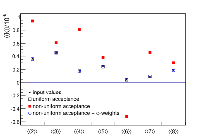
Numerical values on the right-hand side in the above equations were obtained by calculating the theoretical values for each correlator from the Eq. (9), and inserting input values for flow harmonics from (29). We have rescaled observable kdelimited-⟨⟩𝑘\left<k\right> by 10ksuperscript10𝑘10^{-k} in all figures, in order to plot all values on the same scale.
Refer to caption
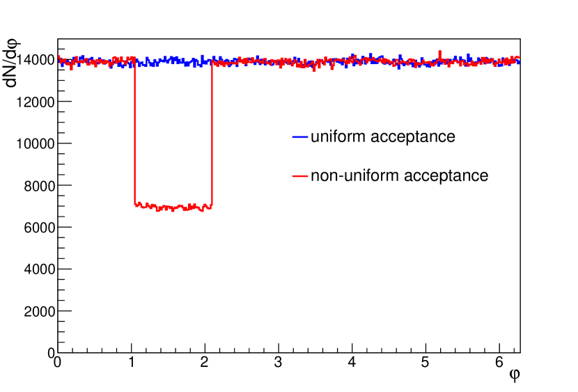
Figure 1: Azimuthal acceptance: uniform (blue)
and non-uniform (red), for a detector.
Refer to caption
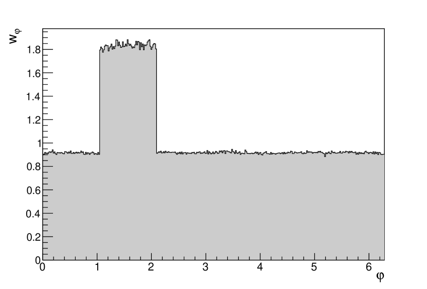
Figure 2: Resulting φ𝜑\varphi-weights for the case of non-uniform azimuthal acceptance shown in Fig. 2.
Refer to caption
Figure 3: Multi-particle observables corrected for non-uniform acceptance using φ𝜑\varphi-weights compared to input values and values for uniform acceptance (see the text for the precise explanation of the ordinate.)

Our toy MC procedure consists of three separate runs. Firstly, we run our simulation for the case of uniform azimuthal acceptance, to demonstrate that the generic equations which we have derived reproduce correctly the input values for all multi-particle observables. This can be seen by comparing filled and open black markers in Fig. 3. Secondly, we have rerun the simulation using the same seed for random generation, but now have selected for analysis each particle with a probability which depends on its azimuthal angle. In particular, the particles which were sampled in the azimuthal range 60oφ<120osuperscript60o𝜑superscript120o60^{\rm o}\leq\varphi<120^{\rm o} have been reduced by 50%percent5050\% for this analysis. In this way we have simulated a non-uniform azimuthal detector acceptance (see Fig. 2), and the corresponding non-negligible systematic bias in anisotropic flow analyses, which is depicted with red filled markers in Fig. 3. In order to correct for this systematic bias, we have constructed φ𝜑\varphi-weights, wφsubscript𝑤𝜑w_{\varphi}, by inverting the histogram for non-uniform acceptance in Fig. 2. The resulting φ𝜑\varphi-weights are shown in Fig. 2. We remark that in our framework the weights do not have to be normalized explicitly, because the analytic equations we provide for multi-particle correlations are normalized by definition (see Eq. (7)). Finally, we rerun the simulation for the third time with the same configuration as in the second run, now utilizing the constructed φ𝜑\varphi-weights from Fig. 2 when we are filling Q𝑄Q-vectors (14) in each event. As can be seen from the blue open circles in Fig. 3, φ𝜑\varphi-weights completely suppress the systematic bias from non-uniform acceptance for all multi-particle observables we have selected in this example.

Based on the previous example, we conclude that as far as φ𝜑\varphi-weights can be constructed for the measured azimuthal distribution, our generic framework can be used to correct for the systematic bias for the cases when that distribution is non-uniform, and it is applicable for any multi-particle observable even when multiple harmonics are present in the system. These two points improve and generalize the prescription outlined in Appendix B of Bilandzic:2010jr . In the next example, we will demonstrate the usage of pTsubscript𝑝Tp_{\rm T}-weights.

IV.2 pTsubscript𝑝Tp_{\rm T}-weights

In this part of the study we use the same MC setup established in the previous example for the φ𝜑\varphi-weights with one exception. In this example we introduce the following pTsubscript𝑝Tp_{\rm T} dependence of v2subscript𝑣2v_{2}:

v2(pT)={v2,max(pT/pcutoff)pT<pcutoffv2,maxpTpcutoff,subscript𝑣2subscript𝑝Tcasessubscript𝑣2maxsubscript𝑝Tsubscript𝑝cutoffsubscript𝑝Tsubscript𝑝cutoffsubscript𝑣2maxsubscript𝑝Tsubscript𝑝cutoffv_{2}(p_{\rm T})=\left\{\begin{array}[]{ll}v_{2,\rm max}(p_{\rm T}/p_{\rm cutoff})&p_{\rm T}<p_{\rm cutoff}\\ v_{2,\rm max}&p_{\rm T}\geq p_{\rm cutoff}\,,\\ \end{array}\right. (32)

and we have set the above parameters to pcutoff=2.0subscript𝑝cutoff2.0p_{\rm cutoff}=2.0 GeV/c𝑐c and v2,max=0.3subscript𝑣2max0.3v_{2,\rm max}=0.3.

Again, we have randomly selected one example for isotropic 2-, 3-, \ldots, and 8-p correlations (suppressing their subscripts for simplicity in the rest of this section):

2delimited-⟨⟩2\displaystyle\left<2\right> \displaystyle\equiv 22,2=v22,subscriptdelimited-⟨⟩222superscriptsubscript𝑣22\displaystyle\left<2\right>_{-2,2}=v_{2}^{2}\,,
3delimited-⟨⟩3\displaystyle\left<3\right> \displaystyle\equiv 35,1,6=v1v5v6,subscriptdelimited-⟨⟩3516subscript𝑣1subscript𝑣5subscript𝑣6\displaystyle\left<3\right>_{-5,-1,6}=v_{1}v_{5}v_{6}\,,
4delimited-⟨⟩4\displaystyle\left<4\right> \displaystyle\equiv 45,2,2,5=v22v52,subscriptdelimited-⟨⟩45225superscriptsubscript𝑣22superscriptsubscript𝑣52\displaystyle\left<4\right>_{-5,-2,2,5}=v_{2}^{2}v_{5}^{2}\,,
5delimited-⟨⟩5\displaystyle\left<5\right> \displaystyle\equiv 55,4,1,4,6=v1v42v5v6,subscriptdelimited-⟨⟩554146subscript𝑣1superscriptsubscript𝑣42subscript𝑣5subscript𝑣6\displaystyle\left<5\right>_{-5,-4,-1,4,6}=v_{1}v_{4}^{2}v_{5}v_{6}\,,
6delimited-⟨⟩6\displaystyle\left<6\right> \displaystyle\equiv 62,2,2,2,3,5=v24v3v5,subscriptdelimited-⟨⟩6222235superscriptsubscript𝑣24subscript𝑣3subscript𝑣5\displaystyle\left<6\right>_{-2,-2,-2,-2,3,5}=v_{2}^{4}v_{3}v_{5}\,,
7delimited-⟨⟩7\displaystyle\left<7\right> \displaystyle\equiv 72,2,2,1,2,2,3=v1v25v3,subscriptdelimited-⟨⟩72221223subscript𝑣1superscriptsubscript𝑣25subscript𝑣3\displaystyle\left<7\right>_{-2,-2,-2,-1,2,2,3}=v_{1}v_{2}^{5}v_{3}\,,
8delimited-⟨⟩8\displaystyle\left<8\right> \displaystyle\equiv 85,4,2,2,2,2,4,5=v24v42v52.subscriptdelimited-⟨⟩854222245superscriptsubscript𝑣24superscriptsubscript𝑣42superscriptsubscript𝑣52\displaystyle\left<8\right>_{-5,-4,-2,-2,2,2,4,5}=v_{2}^{4}v_{4}^{2}v_{5}^{2}\,. (33)

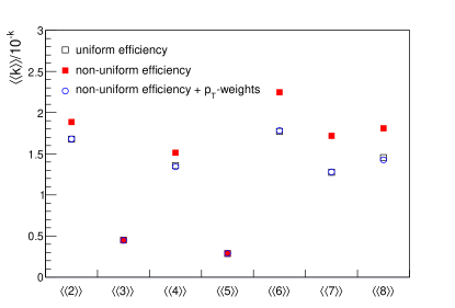
Some of the selected observables (3delimited-⟨⟩delimited-⟨⟩3\left<\left<3\right>\right> and 5delimited-⟨⟩delimited-⟨⟩5\left<\left<5\right>\right>) do not have an explicit dependence on v2subscript𝑣2v_{2}, so we do not expect them to exhibit any systematic bias in this example.

Analogously as in the previous example, our toy MC procedure consists of three separate runs. Firstly, we run our simulation for the case of uniform reconstruction efficiency, in order to obtain the true pTsubscript𝑝Tp_{\rm T} yield; this result is illustrated with the blue line in Fig. 5. Secondly, we have rerun the same simulation, but now have selected for the analysis each particle with a probability which depends on its transverse momentum. The particles in the transverse momentum interval 0.4pT<1.20.4subscript𝑝T1.20.4\leq p_{\rm T}<1.2 have been reduced by 60%percent6060\%. The resulting pTsubscript𝑝Tp_{\rm T} yield is depicted by the red line in Fig. 5. The resulting systematic bias on the selected multi-particle observables (33) can be seen by inspecting the red filled markers in Fig. 6. As already remarked, such a bias is absent in observables 3delimited-⟨⟩delimited-⟨⟩3\left<\left<3\right>\right> and 5delimited-⟨⟩delimited-⟨⟩5\left<\left<5\right>\right>, because they do not have the explicit dependence on the harmonic v2subscript𝑣2v_{2} (see (33)), which is the only harmonic in this study which has a non-trivial pTsubscript𝑝Tp_{\rm T} dependence. To correct for reconstruction efficiency, we have constructed pTsubscript𝑝Tp_{\rm T}-weights, wpTsubscript𝑤subscript𝑝Tw_{p_{\rm T}}, by taking the ratio of the two histograms in Fig. 5. The result is shown in Fig. 5. Finally, in the third run we use the same MC setup as in the second run, only now we make use of the constructed pTsubscript𝑝Tp_{\rm T}-weights from Fig. 5 when filling the Q𝑄Q-vectors (14). The agreement between the results shown with black open squares (uniform efficiency) and the ones shown with blue open circles (non-uniform efficiency using the pTsubscript𝑝Tp_{\rm T}-weights) in Fig. 6, demonstrates clearly that the generic framework is capable of suppressing the systematic bias from non-uniform efficiency for all of the multi-particle observables in question.
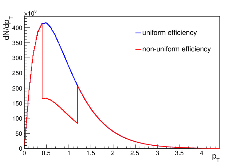
Refer to caption
Figure 4: Transverse momentum yield, with uniform (blue)
and non-uniform (red) reconstruction efficiency.
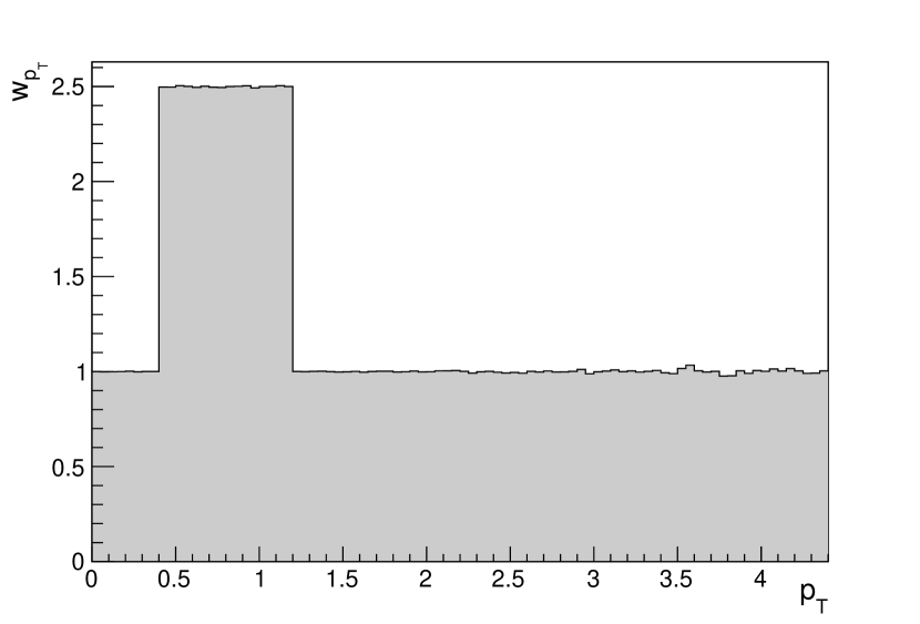
Refer to caption
Figure 5: Resulting pTsubscript𝑝Tp_{\rm T}-weights corresponding to the non-uniform efficiency shown in Fig. 5.
Refer to caption
Figure 6: Results from a toy MC simulation for multi-particle observables corrected for non-uniform efficiency using pTsubscript𝑝Tp_{\rm T}-weights.

With the previous two examples we have demonstrated that, in a simple toy MC study, our generic framework can be utilized to correct for various detector inefficiencies. Next, we will illustrate, in a study based on a realistic MC model, its use in the measurement of some new physical observables which we now propose.

IV.3 Example new observables: “Standard candles”

We now introduce a new type of observable for anisotropic flow analyses, the so-called standard candles (SC), which can be measured with the generic framework we have presented in the previous sections. This observable is particularly useful for systems in which flow harmonics fluctuate in magnitude event-by-event (the case we have in reality). We start with the following generic four-particle correlation:

cos(mφ1+nφ2mφ3nφ4),delimited-⟨⟩delimited-⟨⟩𝑚subscript𝜑1𝑛subscript𝜑2𝑚subscript𝜑3𝑛subscript𝜑4\left<\left<\cos(m\varphi_{1}\!+\!n\varphi_{2}\!-\!m\varphi_{3}-\!n\varphi_{4})\right>\right>\,, (34)

and we impose the constraint mn𝑚𝑛m\neq n. The isotropic part of corresponding four-particle cumulant is given by:

cos(mφ1+nφ2mφ3nφ4)csubscriptdelimited-⟨⟩delimited-⟨⟩𝑚subscript𝜑1𝑛subscript𝜑2𝑚subscript𝜑3𝑛subscript𝜑4𝑐\displaystyle\left<\left<\cos(m\varphi_{1}\!+\!n\varphi_{2}\!-\!m\varphi_{3}-\!n\varphi_{4})\right>\right>_{c} =\displaystyle= cos(mφ1+nφ2mφ3nφ4)delimited-⟨⟩delimited-⟨⟩𝑚subscript𝜑1𝑛subscript𝜑2𝑚subscript𝜑3𝑛subscript𝜑4\displaystyle\left<\left<\cos(m\varphi_{1}\!+\!n\varphi_{2}\!-\!m\varphi_{3}-\!n\varphi_{4})\right>\right> (35)
cos[m(φ1φ2)]cos[n(φ1φ2)]delimited-⟨⟩delimited-⟨⟩𝑚subscript𝜑1subscript𝜑2delimited-⟨⟩delimited-⟨⟩𝑛subscript𝜑1subscript𝜑2\displaystyle{}-\left<\left<\cos[m(\varphi_{1}\!-\!\varphi_{2})]\right>\right>\left<\left<\cos[n(\varphi_{1}\!-\!\varphi_{2})]\right>\right>
=\displaystyle= vm2vn2vm2vn2delimited-⟨⟩superscriptsubscript𝑣𝑚2superscriptsubscript𝑣𝑛2delimited-⟨⟩superscriptsubscript𝑣𝑚2delimited-⟨⟩superscriptsubscript𝑣𝑛2\displaystyle\left<v_{m}^{2}v_{n}^{2}\right>-\left<v_{m}^{2}\right>\left<v_{n}^{2}\right>
=\displaystyle= 0,0\displaystyle 0\,,

where double angular brackets indicate that the averaging from definition (7) has been extended to all events. Due to the condition that mn𝑚𝑛m\neq n, a lot of terms which appear in the general cumulant expansion, for instance cos(mφ1nφ2)delimited-⟨⟩delimited-⟨⟩𝑚subscript𝜑1𝑛subscript𝜑2\left<\left<\cos(m\varphi_{1}\!-\!n\varphi_{2})\right>\right>, are non-isotropic and, therefore, average to zero for a detector with uniform acceptance when the averaging is extended to all events. For fixed values of vmsubscript𝑣𝑚v_{m} and vnsubscript𝑣𝑛v_{n} over all events, the four-particle cumulant as defined in Eq. (35), is zero by definition. Any dependence on the symmetry planes ΨmsubscriptΨ𝑚\Psi_{m} and ΨnsubscriptΨ𝑛\Psi_{n} is also canceled by definition. We can get the result in the last line of Eq. (35) not only when vmsubscript𝑣𝑚v_{m} and vnsubscript𝑣𝑛v_{n} are fixed for all events, but also when event-by-event fluctuations of vmsubscript𝑣𝑚v_{m} and vnsubscript𝑣𝑛v_{n} are uncorrelated, since the expression vm2vn2delimited-⟨⟩superscriptsubscript𝑣𝑚2superscriptsubscript𝑣𝑛2\left<v_{m}^{2}v_{n}^{2}\right> can then be factorized. Taking all these statements into account, the four-particle cumulant (35) is non-zero only if the event-by-event fluctuations of vmsubscript𝑣𝑚v_{m} and vnsubscript𝑣𝑛v_{n} are correlated. Therefore, by measuring the observable (35) we can conclude whether finding vmsubscript𝑣𝑚v_{m} larger than vmdelimited-⟨⟩subscript𝑣𝑚\left<v_{m}\right> in an event will enhance or reduce the probability of finding vnsubscript𝑣𝑛v_{n} larger than vndelimited-⟨⟩subscript𝑣𝑛\left<v_{n}\right> in that event, which is not constrained by any measurement performed yet. Since by definition everything cancels out from the observable (35) except the last contribution, namely the correlation of event-by-event fluctuations of vmsubscript𝑣𝑚v_{m} and vnsubscript𝑣𝑛v_{n}, we name it a “standard candle”. Recently, by using different observables and methodology, these correlations between fluctuations of various harmonics have been studied in Niemi:2012aj ; Huo:2013qma .

In this study, the Monte Carlo event generator, A MultiPhase Transport (AMPT) model, has been used. AMPT is a hybrid model consisting of four main parts: the initial conditions, partonic interactions, hadronization, and hadronic rescatterings. The initial conditions, which include the spatial and momentum distributions of minijet partons and soft string excitations, are obtained from the Heavy Ion Jet Interaction Generator (HIJING) Wang:2000bf . The following stage which describes the interactions between partons is modeled by Zhang’s Parton Cascade (ZPC) Zhang:1997ej , which presently includes only two–body scatterings with cross sections obtained from pQCD with screening masses. In AMPT with string melting Lin:2003iq , the transition from partonic to hadronic matter is done through a simple coalescence model, which combines two quarks into mesons and three quarks into baryons Chen:2005mr . To describe the dynamics of the subsequent hadronic stage, a hadronic cascade, which is based on A Relativistic Transport (ART) model Li:1995pra , is used.

Several configurations of the AMPT model have been investigated to better understand the results based on AMPT simulations Zhou:2010us . The partonic interactions can be tweaked by changing the partonic cross section: for RHIC the default value is 10 mb, while using 3 mb generates weaker partonic interactions in ZPC. We can also change the hadronic interactions by controlling the termination time in ART. Setting NTMAX = 3 will turn off the hadronic interactions effectively Zhou:2010us . Good agreement has been observed recently between anisotropic flow measurements and the AMPT Xu:2011fi . Therefore, we calculate multi-particle azimuthal correlations using AMPT simulations with the input parameters suggested in Xu:2011fi at the LHC energy. For RHIC energies we followed the parameters in Chen:2005mr while different configurations have also been used in this study.

In Fig. 7 we see a clear non-zero value for both SC4,2,4,2𝑆subscript𝐶4242SC_{4,2,-4,-2} (red markers) and SC3,2,3,2𝑆subscript𝐶3232SC_{3,2,-3,-2} (black markers) at the LHC energy. The positive results of SC4,2,4,2𝑆subscript𝐶4242SC_{4,2,-4,-2} suggest a positive correlation between the event-by-event fluctuations of v2subscript𝑣2v_{2} and v4subscript𝑣4v_{4}, which indicates that finding v2subscript𝑣2v_{2} larger than v2delimited-⟨⟩subscript𝑣2\langle v_{2}\rangle in an event enhances the probability of finding v4subscript𝑣4v_{4} larger than v4delimited-⟨⟩subscript𝑣4\langle v_{4}\rangle in that event. On the other hand, the negative results of SC3,2,3,2𝑆subscript𝐶3232SC_{3,2,-3,-2} predict that finding v2subscript𝑣2v_{2} larger than v2delimited-⟨⟩subscript𝑣2\langle v_{2}\rangle enhances the probability of finding v3subscript𝑣3v_{3} smaller than v3delimited-⟨⟩subscript𝑣3\langle v_{3}\rangle.

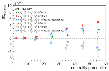
A similar centrality dependence of SC4,2,4,2𝑆subscript𝐶4242SC_{4,2,-4,-2} and SC3,2,3,2𝑆subscript𝐶3232SC_{3,2,-3,-2} is also found at the RHIC energy, see Fig. 8. In addition, we compare the SC4,2,4,2𝑆subscript𝐶4242SC_{4,2,-4,-2} and SC3,2,3,2𝑆subscript𝐶3232SC_{3,2,-3,-2} calculations for three different scenarios: (a) 3 mb; (b) 10 mb; (c) 10 mb, no rescattering. It was shown Zhou:2013 that the relative flow fluctuations of v2subscript𝑣2v_{2} do not depend on the partonic interactions and only relate to the initial eccentricity fluctuations. Therefore, the expectation is that SC4,2,4,2𝑆subscript𝐶4242SC_{4,2,-4,-2} and SC3,2,3,2𝑆subscript𝐶3232SC_{3,2,-3,-2} do not depend on the magnitudes of v2subscript𝑣2v_{2} or v4subscript𝑣4v_{4} (which depend on both partonic interactions and hadronic interactions), but depend only on the initial correlations of event-by-event fluctuations of ε2subscript𝜀2\varepsilon_{2} and ε4subscript𝜀4\varepsilon_{4}. Thus, both SC4,2,4,2𝑆subscript𝐶4242SC_{4,2,-4,-2} and SC3,2,3,2𝑆subscript𝐶3232SC_{3,2,-3,-2} remain the same for different configurations, since the initial state was kept the same each time. However, we find that when the partonic cross section is decreasing from 10 mb (lower shear viscosity, see Xu:2011fi ) to 3 mb (higher shear viscosity), the strength of SC4,2,4,2𝑆subscript𝐶4242SC_{4,2,-4,-2} decreases. Additionally, the ‘10mb, no rescattering’ setup seems to give slightly smaller magnitudes of SC4,2,4,2𝑆subscript𝐶4242SC_{4,2,-4,-2} and SC3,2,3,2𝑆subscript𝐶3232SC_{3,2,-3,-2}.

Considering the AMPT model can quantitatively describe flow measurements at the LHC Xu:2011fi , our AMPT calculations for these new observables provide predictions for the correlations of event-by-event fluctuations of v2subscript𝑣2v_{2} and v4subscript𝑣4v_{4}, and of v2subscript𝑣2v_{2} and v3subscript𝑣3v_{3} for the measurements at the LHC. Such measurements have the potential to shed new light on the underlying physical mechanisms behind flow fluctuations.
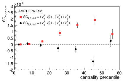
Refer to caption
Figure 7: The centrality dependence of standard candles SC4,2,4,2𝑆subscript𝐶4242SC_{4,2,-4,-2} (red markers) and SC3,2,3,2𝑆subscript𝐶3232SC_{3,2,-3,-2} (black markers) at sNNsubscript𝑠NN\sqrt{s_{\rm NN}} = 2.76 TeV Pb–Pb collisions with AMPT-StringMelting.
Refer to caption
Figure 8: The centrality dependence of standard candles SC4,2,4,2𝑆subscript𝐶4242SC_{4,2,-4,-2} (solid markers) and SC3,2,3,2𝑆subscript𝐶3232SC_{3,2,-3,-2} (open markers) at sNN=subscript𝑠NNabsent\sqrt{s_{\rm NN}}= 200 GeV Au–Au collisions with AMPT-StringMelting. Different scenarios: (a) 3 mb (green circle); (b) 10 mb (red square) and (c) 10 mb, no rescattering (azure star) are presented.

V Detectors with finite granularity

The previous results and examples are applicable only directly to detectors that have infinite resolution. Finite resolution will both bias measurements and cause interference between harmonics. To study this, we define a detector with N𝑁N equal size adjacent azimuthal sectors where the edge of the first sector is shifted from 0 by φΔsubscript𝜑Δ\varphi_{\Delta}. Then the low and high edges of the ithsuperscript𝑖thi^{\mathrm{th}} sector are defined as follows:

φLi=i2πN+φΔ,φHi=(i+1)2πN+φΔ,0iN1.formulae-sequencesubscript𝜑subscript𝐿𝑖𝑖2𝜋𝑁subscript𝜑Δformulae-sequencesubscript𝜑subscript𝐻𝑖𝑖12𝜋𝑁subscript𝜑Δ0𝑖𝑁1\varphi_{L_{i}}=i\frac{2\pi}{N}+\varphi_{\Delta},\qquad\varphi_{H_{i}}=(i+1)\frac{2\pi}{N}+\varphi_{\Delta},\qquad 0\leq i\leq N-1\,. (36)

By integrating Eq. (1) between φLisubscript𝜑subscript𝐿𝑖\varphi_{L_{i}} and φHisubscript𝜑subscript𝐻𝑖\varphi_{H_{i}} (derivation is shown in Appendix B), the probability, Pisubscript𝑃𝑖P_{i}, for a particle to be detected in the ithsuperscript𝑖thi^{\mathrm{th}} sector is found to be:

Pi=1N[1+n=12vnsinnπNnπNcos(n((i+12)2πN+φΔΨn))].subscript𝑃𝑖1𝑁delimited-[]1superscriptsubscript𝑛12subscript𝑣𝑛𝑛𝜋𝑁𝑛𝜋𝑁𝑛𝑖122𝜋𝑁subscript𝜑ΔsubscriptΨ𝑛P_{i}=\frac{1}{N}\left[1+\sum_{n=1}^{\infty}2v_{n}\frac{\sin\frac{n\pi}{N}}{\frac{n\pi}{N}}\cos\left(n\bigg{(}(i+\frac{1}{2})\frac{2\pi}{N}+\varphi_{\Delta}-\Psi_{n}\bigg{)}\right)\right]\,. (37)

The expectation value for an observable for a single particle, θ𝜃\theta, can then be evaluated from Pisubscript𝑃𝑖P_{i} using the following formula:

E[θ]=i=0N1θiPi,𝐸delimited-[]𝜃superscriptsubscript𝑖0𝑁1subscript𝜃𝑖subscript𝑃𝑖E\left[\theta\right]=\sum_{i=0}^{N-1}\theta_{i}P_{i}\,, (38)

where θisubscript𝜃𝑖\theta_{i} is the value of observable evaluated at the center of the sector. It follows that the expectation value of einφsuperscript𝑒𝑖𝑛𝜑e^{in\varphi} (see derivation in Appendix B) is given by:

E[einφ]={(1)nNeinφΔfor nNj=v|jNn|sin(jnN)π(jnN)π(1)jei{(jNn)Ψ|jNn|jNφΔ}for nNE\left[e^{in\varphi}\right]=\left\{\begin{tabular}[]{ll}$(-1)^{\frac{n}{N}}e^{in\varphi_{\Delta}}$&for $\frac{n}{N}\in\mathbb{Z}$\\ $\sum\limits_{j=-\infty}^{\infty}v_{\left|jN-n\right|}\frac{\sin(j-\frac{n}{N})\pi}{(j-\frac{n}{N})\pi}(-1)^{j}e^{-i\left\{(jN-n)\Psi_{\left|jN-n\right|}-jN\varphi_{\Delta}\right\}}$&for $\frac{n}{N}\notin\mathbb{Z}$\end{tabular}\right. (39)

where \mathbb{Z} is the set of all integers. It is evident from this formula that it is not possible to measure any harmonic which is a multiple of the number of sectors. If 0<n<N/20𝑛𝑁20<n<N/2 and the harmonics above N/2𝑁2N/2 can be neglected, Eq. (39) becomes:

E[einφ]vneinΨnsinnNπnNπ.𝐸delimited-[]superscript𝑒𝑖𝑛𝜑subscript𝑣𝑛superscript𝑒𝑖𝑛subscriptΨ𝑛𝑛𝑁𝜋𝑛𝑁𝜋E\left[e^{in\varphi}\right]\approx v_{n}e^{in\Psi_{n}}\frac{\sin\frac{n}{N}\pi}{\frac{n}{N}\pi}\,. (40)

In this case, the multi-particle azimuthal correlations defined in Eq. (7) become (under the assumption (3) of a factorizable p.d.f.):

E[mn1,,nm]k=1mvnkeinkΨnksinnkNπnkNπ.𝐸delimited-[]subscriptdelimited-⟨⟩𝑚subscript𝑛1subscript𝑛𝑚superscriptsubscriptproduct𝑘1𝑚subscript𝑣subscript𝑛𝑘superscript𝑒𝑖subscript𝑛𝑘subscriptΨsubscript𝑛𝑘subscript𝑛𝑘𝑁𝜋subscript𝑛𝑘𝑁𝜋E\left[\left<m\right>_{n_{1},\ldots,n_{m}}\right]\approx\prod_{k=1}^{m}v_{n_{k}}e^{in_{k}\Psi_{n_{k}}}\frac{\sin\frac{n_{k}}{N}\pi}{\frac{n_{k}}{N}\pi}\,. (41)

In this way, the term (nNπ)/sin(nNπ)𝑛𝑁𝜋𝑛𝑁𝜋\left(\frac{n}{N}\pi\right)/\sin\left(\frac{n}{N}\pi\right) is a correction factor for a bias from finite granularity that must be applied for each harmonic that the multi-particle correlator is composed of due to an overall reduction in the measured value.

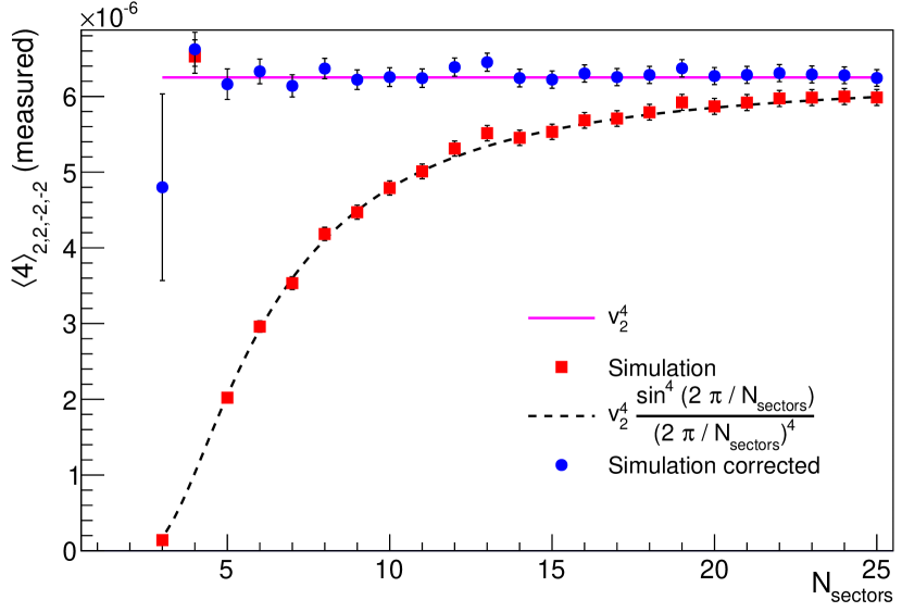
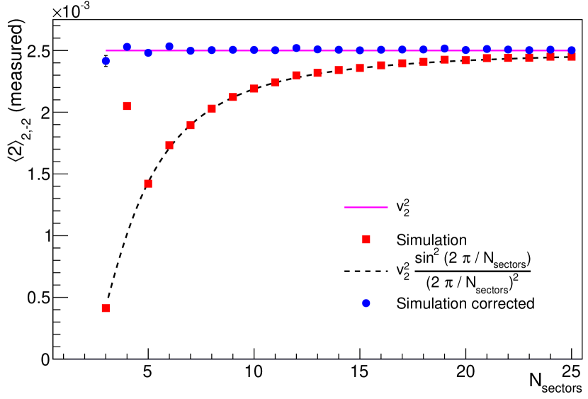
Figure 9 shows the result obtained by calculating 22,2subscriptdelimited-⟨⟩222\langle 2\rangle_{2,-2} and 42,2,2,2subscriptdelimited-⟨⟩42222\langle 4\rangle_{2,2,-2,-2} for detectors with various segmentations, and when the toy Fourier-like p.d.f. was parametrized only with the single harmonic v2subscript𝑣2v_{2}. The simulated values lie on the dashed line suppressed by 2 or 4 factors of sin(2Nπ)/(2Nπ)2𝑁𝜋2𝑁𝜋\sin\left(\frac{2}{N}\pi\right)/\left(\frac{2}{N}\pi\right) (see Eq. (41)). In this case (if N>2𝑁2N>2), the values can be corrected to reproduce the input values of v22superscriptsubscript𝑣22v_{2}^{2} or v24superscriptsubscript𝑣24v_{2}^{4}. The ‘blip’ at N=4𝑁4N=4 is a special case where multiple factors proportional to v2subscript𝑣2v_{2} in Eq. (39) contribute making the measured value 2 times bigger for 22,2subscriptdelimited-⟨⟩222\langle 2\rangle_{2,-2} and 6 times bigger for 42,2,2,2subscriptdelimited-⟨⟩42222\langle 4\rangle_{2,2,-2,-2} than the expected suppressed value (the black dashed line) when averaging over all events.
Refer to caption
Refer to caption
Figure 9: 22,2subscriptdelimited-⟨⟩222\langle 2\rangle_{2,-2} and 42,2,2,2subscriptdelimited-⟨⟩42222\langle 4\rangle_{2,2,-2,-2} (left and right, respectively) evaluated for a range of sectors when only v2subscript𝑣2v_{2} exists (red squares). The magenta line shows the input value of v22superscriptsubscript𝑣22v_{2}^{2} or v24superscriptsubscript𝑣24v_{2}^{4}. The black dashed line shows the expected measured value of the correlator. The blue circles are the simulated values corrected for the reduction to the measured value due to finite granularity.

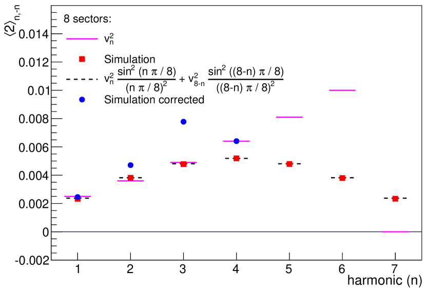
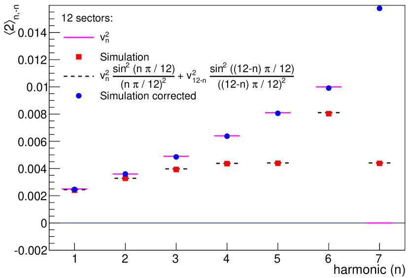
If harmonics above N/2𝑁2N/2 are significant, Eq. (39) shows that finite segmentation will introduce an interference from other harmonics (in fact, from an infinite number of harmonics). If one, for example, considers the case where the first N𝑁N harmonics are non-zero, there will be a contribution from 2 terms in Eq. (39). As an example, we will once again consider the case of the p.d.f in Eq. (28) where the values of the first 6 harmonics are as in Eq. (29). In general if one considers the case where the first N𝑁N harmonics are non-zero, then Eq. (39) produces the following relationship for 2n,nsubscriptdelimited-⟨⟩2𝑛𝑛\langle 2\rangle_{n,-n} when a factorizable p.d.f. (3) exists and one averages over many events:

E[2n,n]=vn2sin2(nπN)(nπN)2+vNn2sin2((nN)πN)((nN)πN)2=E[2Nn,nN].𝐸delimited-[]subscriptdelimited-⟨⟩2𝑛𝑛superscriptsubscript𝑣𝑛2superscript2𝑛𝜋𝑁superscript𝑛𝜋𝑁2superscriptsubscript𝑣𝑁𝑛2superscript2𝑛𝑁𝜋𝑁superscript𝑛𝑁𝜋𝑁2𝐸delimited-[]subscriptdelimited-⟨⟩2𝑁𝑛𝑛𝑁E\left[\left<2\right>_{n,-n}\right]=v_{n}^{2}\frac{\sin^{2}\left(\frac{n\pi}{N}\right)}{\left(\frac{n\pi}{N}\right)^{2}}+v_{N-n}^{2}\frac{\sin^{2}\left(\frac{\left(n-N\right)\pi}{N}\right)}{\left(\frac{\left(n-N\right)\pi}{N}\right)^{2}}=E\left[\left<2\right>_{N-n,n-N}\right]\,. (42)

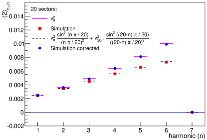
The harmonic vNnsubscript𝑣𝑁𝑛v_{N-n}, therefore, contaminates the measurement of vnsubscript𝑣𝑛v_{n}, although the harmonic below N/2𝑁2N/2 is dominant (i.e. is suppressed less). For low segmentation, this can cause significant interference from other harmonics. If one tries to compute v2subscript𝑣2v_{2} with 8 sectors, for instance, then vNnsubscript𝑣𝑁𝑛v_{N-n} corresponds to v6subscript𝑣6v_{6} which contaminates the v2subscript𝑣2v_{2} calculation. Eq. (42) also explains the origin of the ‘blip’ at n=N/2𝑛𝑁2n=N/2 in Fig. 9, where both terms are proportional to the same harmonic. Figure 10 shows this interference for a detector with 8, 12, and 20 azimuthal sectors. For 8 sectors, only 24,4subscriptdelimited-⟨⟩244\langle 2\rangle_{4,-4} can be corrected for. All other harmonics are contaminated and it is easily seen that 21,1=27,7subscriptdelimited-⟨⟩211subscriptdelimited-⟨⟩277\langle 2\rangle_{1,-1}=\langle 2\rangle_{7,-7}, 22,2=26,6subscriptdelimited-⟨⟩222subscriptdelimited-⟨⟩266\langle 2\rangle_{2,-2}=\langle 2\rangle_{6,-6}, and 23,3=25,5subscriptdelimited-⟨⟩233subscriptdelimited-⟨⟩255\langle 2\rangle_{3,-3}=\langle 2\rangle_{5,-5} for the measured values. These cases cannot be corrected for. However, unless the high harmonics are larger than the lower ones, the measured value will be closest to the lowest harmonic (in the example v1subscript𝑣1v_{1} could be corrected exactly only because v7subscript𝑣7v_{7} was 0 in our toy MC study (29)). For 12 sectors, all of the existing harmonics can be calculated (and corrected for finite granularity). However, v72superscriptsubscript𝑣72v_{7}^{2} is still calculated incorrectly because it is actually measuring v12superscriptsubscript𝑣12v_{1}^{2}. For the case of 20 sectors, all contaminations have disappeared and one can accurately determine the harmonics. In general, one can only measure up to vN/2subscript𝑣𝑁2v_{N/2} and one should have a reasonable estimate of the size of the other harmonics to determine if the contamination from harmonics with n>N/2𝑛𝑁2n>N/2 will be significant.

Refer to caption
Refer to caption
Refer to caption
Figure 10: The measured values of 2n,nsubscriptdelimited-⟨⟩2𝑛𝑛\langle 2\rangle_{n,-n} when the first 6 harmonics exist for detectors with 8, 12, and 20 sectors are shown (red squares). The values of the input harmonics squared are represented by the magenta lines. The black dashed lines show the expected measured value with that number of sectors. The blue circles show the result obtained when correcting for the reduction to the measured value for the harmonic being measured.

VI Systematic bias due to particle selection criteria

In this section we discuss our final topic which concerns the results based on multi-particle correlation techniques. In particular, we point out the existence of a systematic bias in traditional differential flow analyses with two- and multi-particle cumulants, which stems solely from the selection criteria applied on reference particles (RP) and on particles of interest (POI), and which is present also in the ideal case when all nonflow correlations are absent. We need two separate groups of particles, RPs and POIs, in the traditional differential flow analyses to get a statistically stable result in the cases where there exists a small number of POIs in a narrow differential bin of interest. The direct evaluation of the multi-particle correlators in Eq. (7) using only POIs would result in statistically unstable results. To circumvent this, Borghini et al proposed in Borghini:2000sa ; Borghini:2001vi to use RPs for all particles except the first in two- and multi-particle correlators, where RPs are selected from some large statistical sample of particles in an event (e.g. from all charged particles). Any dependence of the differential flow of POIs on RPs would then be eliminated by separately evaluating multi-particle correlators by using only RPs and then by explicitly dividing out their corresponding contribution to differential multi-particle correlators, in which only the first particle was restricted to be a POI. For a detailed description of traditional differential flow analyses we refer the reader to Borghini:2000sa ; Borghini:2001vi ; now we quantify the systematic bias which stems solely from the applied selection criteria on RPs and POIs.

Usually it is said that collective anisotropic flow measured with QC{2}𝑄𝐶2QC\{2\} is enhanced by flow fluctuations and QC{4}𝑄𝐶4QC\{4\} is suppressed by flow fluctuations. When only using reference flow it is also easily shown that (for a detailed derivation, see Appendix A in Bilandzic:2012wva ):

v{2}=v+12σv2v,𝑣2delimited-⟨⟩𝑣12superscriptsubscript𝜎𝑣2delimited-⟨⟩𝑣\displaystyle v\{2\}=\langle v\rangle+\frac{1}{2}\frac{\sigma_{v}^{2}}{\langle v\rangle}\,, (43)
v{4}=v12σv2v,𝑣4delimited-⟨⟩𝑣12superscriptsubscript𝜎𝑣2delimited-⟨⟩𝑣\displaystyle v\{4\}=\langle v\rangle-\frac{1}{2}\frac{\sigma_{v}^{2}}{\langle v\rangle}\,, (44)

where vdelimited-⟨⟩𝑣\langle v\rangle is the mean value of the flow moment of interest, and σv2superscriptsubscript𝜎𝑣2\sigma_{v}^{2} the variance of that flow moment. However, in the more generally applied case, where the reference flow is used to obtain a differential flow, the situation becomes more complicated.

VI.1 v{2}superscript𝑣2v^{\prime}\{2\}

The differential 2-particle cumulant estimate, v{2}superscript𝑣2v^{\prime}\{2\}, is obtained as Borghini:2001vi :

v{2}=vvv2.superscript𝑣2delimited-⟨⟩superscript𝑣𝑣delimited-⟨⟩superscript𝑣2v^{\prime}\{2\}=\frac{\langle v^{\prime}v\rangle}{\sqrt{\langle v^{2}\rangle}}\,. (45)

Using vv=vv+ρσvσvdelimited-⟨⟩superscript𝑣𝑣delimited-⟨⟩superscript𝑣delimited-⟨⟩𝑣𝜌subscript𝜎superscript𝑣subscript𝜎𝑣\langle v^{\prime}v\rangle=\langle v^{\prime}\rangle\langle v\rangle+\rho\,\sigma_{v^{\prime}}\sigma_{v}, where ρ𝜌\rho is the correlation coefficient between the reference flow and the differential flow and is defined in the range [1,1]11[-1,1], where specifically ρ=1𝜌1\rho=1 when v𝑣v and vsuperscript𝑣v^{\prime} are perfectly correlated, ρ=0𝜌0\rho=0 when they are uncorrelated, and ρ=1𝜌1\rho=-1 when they are anticorrelated, one can find the following relation assuming σv2/v21much-less-thansuperscriptsubscript𝜎𝑣2superscriptdelimited-⟨⟩𝑣21\sigma_{v}^{2}/\langle v\rangle^{2}\ll 1:

v{2}v(1+ρσvσvvv12σv2v2),superscript𝑣2delimited-⟨⟩superscript𝑣1𝜌subscript𝜎superscript𝑣subscript𝜎𝑣delimited-⟨⟩superscript𝑣delimited-⟨⟩𝑣12superscriptsubscript𝜎𝑣2superscriptdelimited-⟨⟩𝑣2v^{\prime}\{2\}\approx\langle v^{\prime}\rangle\left(1+\rho\frac{\sigma_{v^{\prime}}\sigma_{v}}{\langle v^{\prime}\rangle\langle v\rangle}-\frac{1}{2}\frac{\sigma_{v}^{2}}{\langle v\rangle^{2}}\right)\,, (46)

from which it is seen that v{2}superscript𝑣2v^{\prime}\{2\} can be suppressed by flow fluctuations.

VI.2 v{4}superscript𝑣4v^{\prime}\{4\}

The differential 4-particle cumulant estimate, v{4}superscript𝑣4v^{\prime}\{4\}, is obtained as Borghini:2001vi :

v{4}=vv3+2vvv2(v{4})3.superscript𝑣4delimited-⟨⟩superscript𝑣superscript𝑣32delimited-⟨⟩superscript𝑣𝑣delimited-⟨⟩superscript𝑣2superscript𝑣43v^{\prime}\{4\}=\frac{-\langle v^{\prime}v^{3}\rangle+2\langle v^{\prime}v\rangle\langle v^{2}\rangle}{\left(v\{4\}\right)^{3}}\,. (47)

Using Eq. (44) and Var[f(x)](f(E[x]))2Var[x]𝑉𝑎𝑟delimited-[]𝑓𝑥superscriptsuperscript𝑓𝐸delimited-[]𝑥2𝑉𝑎𝑟delimited-[]𝑥Var\left[f(x)\right]\approx\left(f^{\prime}\left(E[x]\right)\right)^{2}Var[x] one can obtain:

v{4}v(1ρσvσvvv+12σv2v2).superscript𝑣4delimited-⟨⟩superscript𝑣1𝜌subscript𝜎superscript𝑣subscript𝜎𝑣delimited-⟨⟩superscript𝑣delimited-⟨⟩𝑣12superscriptsubscript𝜎𝑣2superscriptdelimited-⟨⟩𝑣2v^{\prime}\{4\}\approx\langle v^{\prime}\rangle\left(1-\rho\frac{\sigma_{v^{\prime}}\sigma_{v}}{\langle v^{\prime}\rangle\langle v\rangle}+\frac{1}{2}\frac{\sigma_{v}^{2}}{\langle v\rangle^{2}}\right)\,. (48)

This is very similar to Eq. (46). Once again it is clear that the bias to the differential flow may not be the same as for the reference flow, an enhancement or a suppression is possible. Three cases are explored in more detail below, while details of the calculations are provided in Appendix C.

VI.3 Specific cases

vsuperscript𝑣v^{\prime} and v𝑣v are perfectly correlated (ρ=1𝜌1\rho=1) and σv/v=σv/vsubscript𝜎superscript𝑣superscript𝑣subscript𝜎𝑣𝑣\sigma_{v^{\prime}}/v^{\prime}=\sigma_{v}/v. For this case, RPs and POIs can have a full overlap, but it is not required. Eq. (46) can be written as:

v{2}v(1+σv2v212σv2v2)=v(1+12σv2v2).superscript𝑣2delimited-⟨⟩superscript𝑣1superscriptsubscript𝜎superscript𝑣2superscriptdelimited-⟨⟩superscript𝑣212superscriptsubscript𝜎superscript𝑣2superscriptdelimited-⟨⟩superscript𝑣2delimited-⟨⟩superscript𝑣112superscriptsubscript𝜎superscript𝑣2superscriptdelimited-⟨⟩superscript𝑣2v^{\prime}\{2\}\approx\langle v^{\prime}\rangle\left(1+\frac{\sigma_{v^{\prime}}^{2}}{\langle v^{\prime}\rangle^{2}}-\frac{1}{2}\frac{\sigma_{v^{\prime}}^{2}}{\langle v^{\prime}\rangle^{2}}\right)=\langle v^{\prime}\rangle\left(1+\frac{1}{2}\frac{\sigma_{v^{\prime}}^{2}}{\langle v^{\prime}\rangle^{2}}\right)\,. (49)

This case reduces to the regular case where QC{2}𝑄𝐶2QC\{2\} is systematically enhanced by flow fluctuations, just as for the reference flow. Since v{4}superscript𝑣4v^{\prime}\{4\} simply has opposite signs on the fluctuation terms, it follows that in this case it is suppressed, once again the same as the reference flow.

vsuperscript𝑣v^{\prime} and v𝑣v are uncorrelated (ρ=0𝜌0\rho=0). In reality this covers a case where the RPs or POIs are chosen from a two groups of particles that do not overlap and do not contain the same underlying correlations. For this case ρ=0𝜌0\rho=0, so Eq. (46) trivially turns into:

v{2}v(112σv2v2).superscript𝑣2delimited-⟨⟩superscript𝑣112superscriptsubscript𝜎𝑣2superscriptdelimited-⟨⟩𝑣2v^{\prime}\{2\}\approx\langle v^{\prime}\rangle\left(1-\frac{1}{2}\frac{\sigma_{v}^{2}}{\langle v\rangle^{2}}\right)\,. (50)

This means the differential 2-particle cumulant is systematically suppressed by the flow fluctuations in the reference flow, and that the 4-particle differential cumulant is systematically enhanced. Fluctuations from the POIs do not play any role.

vsuperscript𝑣v^{\prime} and v𝑣v are correlated, but the relative fluctuations are different. Once again the RPs and POIs may have a full overlap, but it is not required. In this case it is assumed that ρ1𝜌1\rho\approx 1, leading to:

v{2}v(1+σvσvvv12σv2v2),superscript𝑣2delimited-⟨⟩superscript𝑣1subscript𝜎superscript𝑣subscript𝜎𝑣delimited-⟨⟩superscript𝑣delimited-⟨⟩𝑣12superscriptsubscript𝜎𝑣2superscriptdelimited-⟨⟩𝑣2v^{\prime}\{2\}\approx\langle v^{\prime}\rangle\left(1+\frac{\sigma_{v^{\prime}}\sigma_{v}}{\langle v^{\prime}\rangle\langle v\rangle}-\frac{1}{2}\frac{\sigma_{v}^{2}}{\langle v\rangle^{2}}\right)\,, (51)

and the observed bias for the 2-particle (4-particle) differential cumulant is an enhancement (suppression) as long as 2(σvv)>(σvv)2subscript𝜎superscript𝑣delimited-⟨⟩superscript𝑣subscript𝜎𝑣delimited-⟨⟩𝑣2\left(\frac{\sigma_{v^{\prime}}}{\langle v^{\prime}\rangle}\right)>\left(\frac{\sigma_{v}}{\langle v\rangle}\right). In general the bias observed in the differential flow is influenced by the fluctuations in the reference flow.
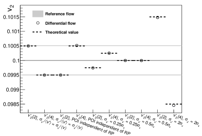
Refer to caption
Figure 11: 106superscript10610^{6} events with 10000 RPs and 1000 POIs. Input flow is v2=0.1subscript𝑣20.1v_{2}=0.1, reference flow fluctuations have σv2=0.01subscript𝜎subscript𝑣20.01\sigma_{v_{2}}=0.01. Depending on the choice of particles for differential flow and the differential flow fluctuations, it is possible to get very different biases to the 2- and 4-particle cumulants.

To illustrate the different cases a simulation of 106superscript10610^{6} events with 10000 RPs and 1000 POIs has been made. The results are shown in Fig. 11 with input values, v2=0.1subscript𝑣20.1v_{2}=0.1 and σv2=0.01subscript𝜎subscript𝑣20.01\sigma_{v_{2}}=0.01. In the figure Gaussian fluctuations are assumed, but other fluctuations, e.g., uniform fluctuations, would yield similar results. The shaded bands indicate the reference flow of v{2}𝑣2v\{2\} and v{4}𝑣4v\{4\}, calculated with Eqs. (43) and (44) respectively, showing the usual enhancement or suppression. The first two points are from a simulation illustrating the first case above, where the POIs and RPs are perfectly correlated and share the same relative fluctuations and have a full overlap. The dotted lines are calculated using Eq. (49) for QC{2}𝑄𝐶2QC\{2\} and the corresponding equation for QC{4}𝑄𝐶4QC\{4\}. For the next two points the POIs and RPs are chosen with independent fluctuations and no overlap. In this case v{2}superscript𝑣2v^{\prime}\{2\} and v{4}superscript𝑣4v^{\prime}\{4\} are swapped, as expected from Eq. (50). The last points show cases where the relative fluctuations in the POIs differ from those in the RPs, this can cause the usual enhancement and suppression to be larger, swapped or even be removed completely, depending on how the relative fluctuations are chosen. In the example simulations shown here, RPs and POIs do not overlap. For the case where σv=0.25σvsubscript𝜎superscript𝑣0.25subscript𝜎𝑣\sigma_{v^{\prime}}=0.25\sigma_{v} Eq. (51) yields:

v{24}=v(114σv2v2).superscript𝑣24delimited-⟨⟩superscript𝑣minus-or-plus114superscriptsubscript𝜎𝑣2superscriptdelimited-⟨⟩𝑣2v^{\prime}\{\begin{subarray}{c}2\\ 4\end{subarray}\}=\langle v^{\prime}\rangle\left(1\mp\frac{1}{4}\frac{\sigma_{v}^{2}}{\langle v\rangle^{2}}\right)\,. (52)

For σv=0.5σvsubscript𝜎superscript𝑣0.5subscript𝜎𝑣\sigma_{v^{\prime}}=0.5\sigma_{v} Eq. (51) yields:

v{24}=v,superscript𝑣24delimited-⟨⟩superscript𝑣v^{\prime}\{\begin{subarray}{c}2\\ 4\end{subarray}\}=\langle v^{\prime}\rangle\,, (53)

and finally for σv=2σvsubscript𝜎superscript𝑣2subscript𝜎𝑣\sigma_{v^{\prime}}=2\sigma_{v}:

v{24}=v(1±32σv2v2).superscript𝑣24delimited-⟨⟩superscript𝑣plus-or-minus132superscriptsubscript𝜎𝑣2superscriptdelimited-⟨⟩𝑣2v^{\prime}\{\begin{subarray}{c}2\\ 4\end{subarray}\}=\langle v^{\prime}\rangle\left(1\pm\frac{3}{2}\frac{\sigma_{v}^{2}}{\langle v\rangle^{2}}\right)\,. (54)

It is tempting to use Eqs. (43) and (44) to estimate the magnitude of the flow fluctuations. However, when doing differential flow analysis with cumulants it is clear from Eqs. (46) and (48) that it may not be feasible. In fact, any analysis using differential flow should be very careful to describe the choice of RPs and POIs in great detail, such that comparison between different experiments and theories is not biased by mixing two or more of the cases shown in Fig. 11 and described above.

VII Summary

We have presented the new generic framework within which all multi-particle azimuthal correlations can be evaluated analytically, with a fast single pass over the particles, free from autocorrelations by definition, and corrected for systematic biases due the various detector inefficiencies. For higher order correlators the direct implementation of analytic solutions is not feasible due to their size; this issue was resolved with the development of new recursive algorithms. We have proposed new multi-particle observables to be used in anisotropic flow analyses (standard candles) which can be measured for the first time within our generic framework. The systematic biases due to finite granularity of detector on multi-particle correlators have been quantified. We have pointed out the existence of a systematic bias characteristic for traditional differential flow analyses when all particles are divided into two groups of reference particles (RP) and particles of interest (POI), which originates solely from the selection criteria for RPs and POIs, and which is present also in the ideal case when all nonflow correlations are absent. Finally, we have straightforwardly generalized our generic framework to the case of differential multi-particle correlators.

Acknowledgements.
We thank Jens Jørgen Gaardhøje for carefully reading the paper and providing valuable feedback for its improvement. We thank Jean-Yves Ollitrault and Sergei Voloshin for important suggestions in the historical account on multi-particle correlation techniques presented in the Introduction. We appreciate help and cheerful discussions from Marek Chojnacki in the derivation of recursive algorithms. We thank Jiangyong Jia for valuable feedback on the studies of correlations of event-by-event fluctuations of various harmonics. We thank the Danish Council for Independent Research, Natural Sciences and the Danish National Research Foundation (Danmarks Grundforskningsfond) for support. This work is also supported by FOM and NWO of the Netherlands.

Appendix A Recursive algorithm

As mentioned in Section III.1, we provide implementations CHC for calculating generic multi-particle correlators defined in Eq. (7) for:

Fully expanded

expressions for Nmn1,,nmNsubscriptdelimited-⟨⟩𝑚subscript𝑛1subscript𝑛𝑚\mathrm{N}\langle m\rangle_{n_{1},\ldots,n_{m}} (see (16) and (19-22)) for m=2,,8𝑚28m=2,\ldots,8;

Recurrence

expression Nmn1,,nmNsuperscriptsubscriptdelimited-⟨⟩𝑚subscript𝑛1subscript𝑛𝑚\mathrm{N}\langle m\rangle_{n_{1},\ldots,n_{m}}^{\prime} (see (III.1)) for any m𝑚m;

Recursive

expression Nmn1,,nm′′Nsuperscriptsubscriptdelimited-⟨⟩𝑚subscript𝑛1subscript𝑛𝑚′′\mathrm{N}\langle m\rangle_{n_{1},\ldots,n_{m}}^{\prime\prime} (see (III.1)) for any m𝑚m.

The largest feasible m𝑚m for the two latter methods above is of course limited by computing time, resources and machine precision. However, there is no inherent limitations on m𝑚m in the implementations.

The implementation is done in plain callable C++ with no external dependencies. It can be integrated into any existing framework, including ROOT ROOT based ones, by simple inclusion of the appropriate headers. Examples of standalone and ROOT applications are provided in the code. The code itself is further heavily documented at CHC .

The choice of method, using either expanded, recurrence, or recursive expression, is left to the user. However, it should be noted, that using the truly general recurrence, or recursive expressions does incur a performance penalty, as can be seen from Fig. 12.
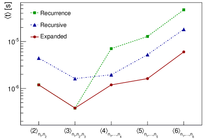
Refer to caption
Figure 12: Average computation time (in seconds) of multi-particle correlators for the three methods as a function of correlator order m𝑚m: Fully expanded are red circles, recurrence are green squares, and recursive are blue triangles.

Appendix B Finite granularity

In this appendix, the equations used in Section V to evaluate the effects of finite granularity are derived. We start by defining a detector with N𝑁N equal size adjacent azimuthal sectors with sectors being labeled by an integer i𝑖i where 0iN10𝑖𝑁10\leq i\leq N-1. Furthermore the low edge of the first sector is shifted from 0 by φΔsubscript𝜑Δ\varphi_{\Delta}. The edges of sector i𝑖i are then defined by:

φLi=i2πN+φΔ,φHi=(i+1)2πN+φΔ.formulae-sequencesubscript𝜑subscript𝐿𝑖𝑖2𝜋𝑁subscript𝜑Δsubscript𝜑subscript𝐻𝑖𝑖12𝜋𝑁subscript𝜑Δ\varphi_{L_{i}}=i\frac{2\pi}{N}+\varphi_{\Delta},\qquad\varphi_{H_{i}}=(i+1)\frac{2\pi}{N}+\varphi_{\Delta}\,. (55)

The p.d.f. for any particle is taken to be:

dPdφ=12π[1+n=12vncos(n(φΨn))].𝑑𝑃𝑑𝜑12𝜋delimited-[]1superscriptsubscript𝑛12subscript𝑣𝑛𝑛𝜑subscriptΨ𝑛\frac{dP}{d\varphi}=\frac{1}{2\pi}\left[1+\sum_{n=1}^{\infty}2v_{n}\cos\left(n\left(\varphi-\Psi_{n}\right)\right)\right]\,. (56)

The probability of a particle going into sector i𝑖i is then found by integrating over the limits of the sector:

Pisubscript𝑃𝑖\displaystyle P_{i} =φLiφHidPdφ𝑑φabsentsuperscriptsubscriptsubscript𝜑subscript𝐿𝑖subscript𝜑subscript𝐻𝑖𝑑𝑃𝑑𝜑differential-d𝜑\displaystyle=\int_{\varphi_{L_{i}}}^{\varphi_{H_{i}}}\frac{dP}{d\varphi}d\varphi =12π[φLiφHi𝑑φ+n=12vnφLiφHicos(n(φΨn))𝑑φ]absent12𝜋delimited-[]superscriptsubscriptsubscript𝜑subscript𝐿𝑖subscript𝜑subscript𝐻𝑖differential-d𝜑superscriptsubscript𝑛12subscript𝑣𝑛superscriptsubscriptsubscript𝜑subscript𝐿𝑖subscript𝜑subscript𝐻𝑖𝑛𝜑subscriptΨ𝑛differential-d𝜑\displaystyle=\frac{1}{2\pi}\left[\int_{\varphi_{L_{i}}}^{\varphi_{H_{i}}}d\varphi+\sum_{n=1}^{\infty}2v_{n}\int_{\varphi_{L_{i}}}^{\varphi_{H_{i}}}\cos\left(n\left(\varphi-\Psi_{n}\right)\right)d\varphi\right] (57)
=12π[2πN+n=12vnsin(n(φLiΨn))sin(n(φHiΨn))n]absent12𝜋delimited-[]2𝜋𝑁superscriptsubscript𝑛12subscript𝑣𝑛𝑛subscript𝜑subscript𝐿𝑖subscriptΨ𝑛𝑛subscript𝜑subscript𝐻𝑖subscriptΨ𝑛𝑛\displaystyle=\frac{1}{2\pi}\left[\frac{2\pi}{N}+\sum_{n=1}^{\infty}2v_{n}\frac{\sin\left(n\left(\varphi_{L_{i}}-\Psi_{n}\right)\right)-\sin\left(n\left(\varphi_{H_{i}}-\Psi_{n}\right)\right)}{n}\right]
=12π[2πN+n=12vn2sin(n(φHiφLi)2)cos(n(φHi+φLi2Ψn))n]absent12𝜋delimited-[]2𝜋𝑁superscriptsubscript𝑛12subscript𝑣𝑛2𝑛subscript𝜑subscript𝐻𝑖subscript𝜑subscript𝐿𝑖2𝑛subscript𝜑subscript𝐻𝑖subscript𝜑subscript𝐿𝑖2subscriptΨ𝑛𝑛\displaystyle=\frac{1}{2\pi}\left[\frac{2\pi}{N}+\sum_{n=1}^{\infty}2v_{n}\frac{2\sin\left(n\frac{\left(\varphi_{H_{i}}-\varphi_{L_{i}}\right)}{2}\right)\cos\left(n\left(\frac{\varphi_{H_{i}}+\varphi_{L_{i}}}{2}-\Psi_{n}\right)\right)}{n}\right]
=1N[1+n=12vnsin(n(φHiφLi)2)nπNcos(n(φHi+φLi2Ψn))]absent1𝑁delimited-[]1superscriptsubscript𝑛12subscript𝑣𝑛𝑛subscript𝜑subscript𝐻𝑖subscript𝜑subscript𝐿𝑖2𝑛𝜋𝑁𝑛subscript𝜑subscript𝐻𝑖subscript𝜑subscript𝐿𝑖2subscriptΨ𝑛\displaystyle=\frac{1}{N}\left[1+\sum_{n=1}^{\infty}2v_{n}\frac{\sin\left(n\frac{\left(\varphi_{H_{i}}-\varphi_{L_{i}}\right)}{2}\right)}{\frac{n\pi}{N}}\cos\left(n\left(\frac{\varphi_{H_{i}}+\varphi_{L_{i}}}{2}-\Psi_{n}\right)\right)\right]
=1N[1+n=12vnsinnπNnπNcos(n((i+12)2πN+φΔΨn))].absent1𝑁delimited-[]1superscriptsubscript𝑛12subscript𝑣𝑛𝑛𝜋𝑁𝑛𝜋𝑁𝑛𝑖122𝜋𝑁subscript𝜑ΔsubscriptΨ𝑛\displaystyle=\frac{1}{N}\left[1+\sum_{n=1}^{\infty}2v_{n}\frac{\sin\frac{n\pi}{N}}{\frac{n\pi}{N}}\cos\left(n\left(\left(i+\frac{1}{2}\right)\frac{2\pi}{N}+\varphi_{\Delta}-\Psi_{n}\right)\right)\right]\,.

The expected value of eimφsuperscript𝑒𝑖𝑚𝜑e^{im\varphi} must then be evaluated as follows:

E[eimφ]𝐸delimited-[]superscript𝑒𝑖𝑚𝜑\displaystyle E\left[e^{im\varphi}\right] =\displaystyle= j=0N1eim[(j+12)2πN+φΔ]Pjsuperscriptsubscript𝑗0𝑁1superscript𝑒𝑖𝑚delimited-[]𝑗122𝜋𝑁subscript𝜑Δsubscript𝑃𝑗\displaystyle\sum\limits_{j=0}^{N-1}e^{im\left[\left(j+\frac{1}{2}\right)\frac{2\pi}{N}+\varphi_{\Delta}\right]}P_{j} (58)
=\displaystyle= 1Nj=0N1eim[(j+12)2πN+φΔ]1𝑁superscriptsubscript𝑗0𝑁1superscript𝑒𝑖𝑚delimited-[]𝑗122𝜋𝑁subscript𝜑Δ\displaystyle\frac{1}{N}\sum_{j=0}^{N-1}e^{im\left[(j+\frac{1}{2})\frac{2\pi}{N}+\varphi_{\Delta}\right]}
+1Nn=1vnsinnπNnπN[einΨnj=0N1ei(m+n)[(j+12)2πN+φΔ]+einΨnj=0N1ei(mn)[(j+12)2πN+φΔ]].1𝑁superscriptsubscript𝑛1subscript𝑣𝑛𝑛𝜋𝑁𝑛𝜋𝑁delimited-[]superscript𝑒𝑖𝑛subscriptΨ𝑛superscriptsubscript𝑗0𝑁1superscript𝑒𝑖𝑚𝑛delimited-[]𝑗122𝜋𝑁subscript𝜑Δsuperscript𝑒𝑖𝑛subscriptΨ𝑛superscriptsubscript𝑗0𝑁1superscript𝑒𝑖𝑚𝑛delimited-[]𝑗122𝜋𝑁subscript𝜑Δ\displaystyle{}+\frac{1}{N}\sum_{n=1}^{\infty}v_{n}\frac{\sin\frac{n\pi}{N}}{\frac{n\pi}{N}}\left[e^{-in\Psi_{n}}\sum_{j=0}^{N-1}e^{i(m+n)\left[(j+\frac{1}{2})\frac{2\pi}{N}+\varphi_{\Delta}\right]}+e^{in\Psi_{n}}\sum_{j=0}^{N-1}e^{i(m-n)\left[(j+\frac{1}{2})\frac{2\pi}{N}+\varphi_{\Delta}\right]}\right]\,.

Eq. (58) has terms of the form j=0N1eik[(j+12)2πN+φΔ]superscriptsubscript𝑗0𝑁1superscript𝑒𝑖𝑘delimited-[]𝑗122𝜋𝑁subscript𝜑Δ\sum_{j=0}^{N-1}e^{ik\left[(j+\frac{1}{2})\frac{2\pi}{N}+\varphi_{\Delta}\right]}, where k𝑘k is an integer, that must be evaluated. We can first evaluate the following:

j=0N1ei(j+12)2πkNsuperscriptsubscript𝑗0𝑁1superscript𝑒𝑖𝑗122𝜋𝑘𝑁\displaystyle\sum_{j=0}^{N-1}e^{i(j+\frac{1}{2})\frac{2\pi k}{N}} =\displaystyle= eiπkN+e3iπkN++e(2N3)iπkN+e(2N1)iπkNsuperscript𝑒𝑖𝜋𝑘𝑁superscript𝑒3𝑖𝜋𝑘𝑁superscript𝑒2𝑁3𝑖𝜋𝑘𝑁superscript𝑒2𝑁1𝑖𝜋𝑘𝑁\displaystyle e^{i\frac{\pi k}{N}}+e^{3i\frac{\pi k}{N}}+\ldots+e^{(2N-3)i\frac{\pi k}{N}}+e^{(2N-1)i\frac{\pi k}{N}} (59)
=\displaystyle= eiπkN{1+e2iπkN++e2(N2)iπkN+e2(N1)iπkN}.superscript𝑒𝑖𝜋𝑘𝑁1superscript𝑒2𝑖𝜋𝑘𝑁superscript𝑒2𝑁2𝑖𝜋𝑘𝑁superscript𝑒2𝑁1𝑖𝜋𝑘𝑁\displaystyle e^{i\frac{\pi k}{N}}\left\{1+e^{2i\frac{\pi k}{N}}+\ldots+e^{2(N-2)i\frac{\pi k}{N}}+e^{2(N-1)i\frac{\pi k}{N}}\right\}\,.

If k/N𝑘𝑁k/N\in\mathbb{Z}, where \mathbb{Z} is the set of all integers, then:

j=0N1ei(j+12)2πkNsuperscriptsubscript𝑗0𝑁1superscript𝑒𝑖𝑗122𝜋𝑘𝑁\displaystyle\sum_{j=0}^{N-1}e^{i(j+\frac{1}{2})\frac{2\pi k}{N}} =kNsuperscript𝑘𝑁\displaystyle\stackrel{{\scriptstyle\frac{k}{N}\in\mathbb{Z}}}{{=}} (1)kN{1+1++1+1}superscript1𝑘𝑁1111\displaystyle(-1)^{\frac{k}{N}}\left\{1+1+\ldots+1+1\right\} (60)
=kNsuperscript𝑘𝑁\displaystyle\stackrel{{\scriptstyle\frac{k}{N}\in\mathbb{Z}}}{{=}} N(1)kN.𝑁superscript1𝑘𝑁\displaystyle N(-1)^{\frac{k}{N}}\,.

If k/N𝑘𝑁k/N\notin\mathbb{Z} then the sum can be evaluated as follows:

(1e2πikN)not 0 if kN×j=0N1ei(j+12)2πkN=kNeiπkN(1e2πik)0 since k,superscript𝑘𝑁subscript1superscript𝑒2𝜋𝑖𝑘𝑁not 0 if kNsuperscriptsubscript𝑗0𝑁1superscript𝑒𝑖𝑗122𝜋𝑘𝑁superscript𝑒𝑖𝜋𝑘𝑁subscript1superscript𝑒2𝜋𝑖𝑘0 since k\underbrace{\left(1-e^{2\pi i\frac{k}{N}}\right)}_{\text{not 0 if $\frac{k}{N}\notin\mathbb{Z}$}}\times\sum_{j=0}^{N-1}e^{i(j+\frac{1}{2})\frac{2\pi k}{N}}\stackrel{{\scriptstyle\frac{k}{N}\notin\mathbb{Z}}}{{=}}e^{i\frac{\pi k}{N}}\underbrace{\left(1-e^{2\pi ik}\right)}_{\text{0 since $k\in\mathbb{Z}$}}\,,

which yields:

j=0N1ei(j+12)2πkN=kN0.superscript𝑘𝑁superscriptsubscript𝑗0𝑁1superscript𝑒𝑖𝑗122𝜋𝑘𝑁0\sum_{j=0}^{N-1}e^{i(j+\frac{1}{2})\frac{2\pi k}{N}}\stackrel{{\scriptstyle\frac{k}{N}\notin\mathbb{Z}}}{{=}}0\,. (61)

Therefore the following is true:

j=0N1eik(j+12)2πN={N(1)kNfor kN0for kN\sum_{j=0}^{N-1}e^{ik(j+\frac{1}{2})\frac{2\pi}{N}}=\left\{\begin{tabular}[]{cl}$N(-1)^{\frac{k}{N}}$&for $\frac{k}{N}\in\mathbb{Z}$\\ 0&for $\frac{k}{N}\notin\mathbb{Z}$\end{tabular}\right. (62)

from which it follows:

j=0N1eik[(j+12)2πN+φΔ]={N(1)kNeikφΔfor kN0for kN\sum_{j=0}^{N-1}e^{ik\left[(j+\frac{1}{2})\frac{2\pi}{N}+\varphi_{\Delta}\right]}=\left\{\begin{tabular}[]{cl}$N(-1)^{\frac{k}{N}}e^{ik\varphi_{\Delta}}$&for $\frac{k}{N}\in\mathbb{Z}$\\ 0&for $\frac{k}{N}\notin\mathbb{Z}$\end{tabular}\right. (63)

If we then define the following function:

α(a,b){(1)abfor ab0for ab\alpha(a,b)\equiv\left\{\begin{tabular}[]{cl}$(-1)^{\frac{a}{b}}$&for $\frac{a}{b}\in\mathbb{Z}$\\ 0&for $\frac{a}{b}\notin\mathbb{Z}$\end{tabular}\right. (64)

then Eq. (58) becomes:

E[eimφ]=eimφΔα(m,N)+n=1vnsinnπNnπN[einΨnei(m+n)φΔα(m+n,N)+einΨnei(mn)φΔα(mn,N)].𝐸delimited-[]superscript𝑒𝑖𝑚𝜑superscript𝑒𝑖𝑚subscript𝜑Δ𝛼𝑚𝑁superscriptsubscript𝑛1subscript𝑣𝑛𝑛𝜋𝑁𝑛𝜋𝑁delimited-[]superscript𝑒𝑖𝑛subscriptΨ𝑛superscript𝑒𝑖𝑚𝑛subscript𝜑Δ𝛼𝑚𝑛𝑁superscript𝑒𝑖𝑛subscriptΨ𝑛superscript𝑒𝑖𝑚𝑛subscript𝜑Δ𝛼𝑚𝑛𝑁E\left[e^{im\varphi}\right]=e^{im\varphi_{\Delta}}\alpha(m,N)+\sum_{n=1}^{\infty}v_{n}\frac{\sin\frac{n\pi}{N}}{\frac{n\pi}{N}}\left[e^{-in\Psi_{n}}e^{i\left(m+n\right)\varphi_{\Delta}}\alpha(m+n,N)+e^{in\Psi_{n}}e^{i\left(m-n\right)\varphi_{\Delta}}\alpha(m-n,N)\right]\,. (65)

The terms with α(m+n,N)𝛼𝑚𝑛𝑁\alpha(m+n,N) will have m+n=jN𝑚𝑛𝑗𝑁m+n=jN where j𝑗j is an integer. Values of n𝑛n which produce non-zero contributions must have n=jNm𝑛𝑗𝑁𝑚n=jN-m. Since n>0𝑛0n>0, this means that jNm>0𝑗𝑁𝑚0jN-m>0 and, therefore, j>m/N𝑗𝑚𝑁j>m/N. The following relation is then true:

n=1vnsinnπNnπNeinΨnei(m+n)φΔα(m+n,N)superscriptsubscript𝑛1subscript𝑣𝑛𝑛𝜋𝑁𝑛𝜋𝑁superscript𝑒𝑖𝑛subscriptΨ𝑛superscript𝑒𝑖𝑚𝑛subscript𝜑Δ𝛼𝑚𝑛𝑁\displaystyle\sum_{n=1}^{\infty}v_{n}\frac{\sin\frac{n\pi}{N}}{\frac{n\pi}{N}}e^{-in\Psi_{n}}e^{i\left(m+n\right)\varphi_{\Delta}}\alpha(m+n,N)
=j=j>mNvjNmsin(jNm)πN(jNm)πNei(jNm)ΨjNmeijNφΔ(1)j.absentsuperscriptsubscript𝑗𝑗𝑚𝑁subscript𝑣𝑗𝑁𝑚𝑗𝑁𝑚𝜋𝑁𝑗𝑁𝑚𝜋𝑁superscript𝑒𝑖𝑗𝑁𝑚subscriptΨ𝑗𝑁𝑚superscript𝑒𝑖𝑗𝑁subscript𝜑Δsuperscript1𝑗\displaystyle\hphantom{\sum_{n=1}^{\infty}}=\sum_{\begin{subarray}{c}j=-\infty\\ j>\frac{m}{N}\end{subarray}}^{\infty}v_{jN-m}\frac{\sin\frac{\left(jN-m\right)\pi}{N}}{\frac{\left(jN-m\right)\pi}{N}}e^{-i\left(jN-m\right)\Psi_{jN-m}}e^{ijN\varphi_{\Delta}}(-1)^{j}\,. (66)

The same argument can be made for the α(mn,N)𝛼𝑚𝑛𝑁\alpha(m-n,N) terms where n=mjN𝑛𝑚𝑗𝑁n=m-jN and j<m/N𝑗𝑚𝑁j<m/N giving the following relation:

n=1vnsinnπNnπNeinΨnei(mn)φΔα(mn,N)superscriptsubscript𝑛1subscript𝑣𝑛𝑛𝜋𝑁𝑛𝜋𝑁superscript𝑒𝑖𝑛subscriptΨ𝑛superscript𝑒𝑖𝑚𝑛subscript𝜑Δ𝛼𝑚𝑛𝑁\displaystyle\sum_{n=1}^{\infty}v_{n}\frac{\sin\frac{n\pi}{N}}{\frac{n\pi}{N}}e^{in\Psi_{n}}e^{i\left(m-n\right)\varphi_{\Delta}}\alpha(m-n,N)
=j=j<mNvmjNsin(mjN)πN(mjN)πNei(mjN)ΨmjNeijNφΔ(1)j.absentsuperscriptsubscript𝑗𝑗𝑚𝑁subscript𝑣𝑚𝑗𝑁𝑚𝑗𝑁𝜋𝑁𝑚𝑗𝑁𝜋𝑁superscript𝑒𝑖𝑚𝑗𝑁subscriptΨ𝑚𝑗𝑁superscript𝑒𝑖𝑗𝑁subscript𝜑Δsuperscript1𝑗\displaystyle\hphantom{\sum_{n=1}^{\infty}}=\sum_{\begin{subarray}{c}j=-\infty\\ j<\frac{m}{N}\end{subarray}}^{\infty}v_{m-jN}\frac{\sin\frac{\left(m-jN\right)\pi}{N}}{\frac{\left(m-jN\right)\pi}{N}}e^{i\left(m-jN\right)\Psi_{m-jN}}e^{ijN\varphi_{\Delta}}(-1)^{j}\,. (67)

The two sets of terms can be combined as follows:

n=1vnsinnπNnπN[einΨnei(m+n)φΔα(m+n,N)+einΨnei(mn)φΔα(mn,N)]superscriptsubscript𝑛1subscript𝑣𝑛𝑛𝜋𝑁𝑛𝜋𝑁delimited-[]superscript𝑒𝑖𝑛subscriptΨ𝑛superscript𝑒𝑖𝑚𝑛subscript𝜑Δ𝛼𝑚𝑛𝑁superscript𝑒𝑖𝑛subscriptΨ𝑛superscript𝑒𝑖𝑚𝑛subscript𝜑Δ𝛼𝑚𝑛𝑁\displaystyle\sum_{n=1}^{\infty}v_{n}\frac{\sin\frac{n\pi}{N}}{\frac{n\pi}{N}}\left[e^{-in\Psi_{n}}e^{i\left(m+n\right)\varphi_{\Delta}}\alpha(m+n,N)+e^{in\Psi_{n}}e^{i\left(m-n\right)\varphi_{\Delta}}\alpha(m-n,N)\right]
=j=jmNv|jNm|sin(jmN)π(jmN)π(1)jei(jNm)Ψ|jNm|eijNφΔ.absentsuperscriptsubscript𝑗𝑗𝑚𝑁subscript𝑣𝑗𝑁𝑚𝑗𝑚𝑁𝜋𝑗𝑚𝑁𝜋superscript1𝑗superscript𝑒𝑖𝑗𝑁𝑚subscriptΨ𝑗𝑁𝑚superscript𝑒𝑖𝑗𝑁subscript𝜑Δ\displaystyle\hphantom{\sum_{n=1}^{\infty}}=\sum_{\begin{subarray}{c}j=-\infty\\ j\neq\frac{m}{N}\end{subarray}}^{\infty}v_{\left|jN-m\right|}\frac{\sin\left(j-\frac{m}{N}\right)\pi}{\left(j-\frac{m}{N}\right)\pi}(-1)^{j}e^{-i\left(jN-m\right)\Psi_{\left|jN-m\right|}}e^{ijN\varphi_{\Delta}}\,. (68)

With this relation, Eq. (65) becomes:

E[eimφ]=eimφΔα(m,N)+j=jmNv|jNm|sin(jmN)π(jmN)π(1)jei(jNm)Ψ|jNm|eijNφΔ.𝐸delimited-[]superscript𝑒𝑖𝑚𝜑superscript𝑒𝑖𝑚subscript𝜑Δ𝛼𝑚𝑁superscriptsubscript𝑗𝑗𝑚𝑁subscript𝑣𝑗𝑁𝑚𝑗𝑚𝑁𝜋𝑗𝑚𝑁𝜋superscript1𝑗superscript𝑒𝑖𝑗𝑁𝑚subscriptΨ𝑗𝑁𝑚superscript𝑒𝑖𝑗𝑁subscript𝜑ΔE\left[e^{im\varphi}\right]=e^{im\varphi_{\Delta}}\alpha(m,N)+\sum_{\begin{subarray}{c}j=-\infty\\ j\neq\frac{m}{N}\end{subarray}}^{\infty}v_{\left|jN-m\right|}\frac{\sin\left(j-\frac{m}{N}\right)\pi}{\left(j-\frac{m}{N}\right)\pi}(-1)^{j}e^{-i\left(jN-m\right)\Psi_{\left|jN-m\right|}}e^{ijN\varphi_{\Delta}}\,. (69)

If m𝑚m is a multiple of N𝑁N, every term in the second part of Eq. (69) is 0 either because the term is excluded (jm/N𝑗𝑚𝑁j\neq m/N) or because sin(jm/N)π=0𝑗𝑚𝑁𝜋0\sin(j-m/N)\pi=0. The first term, however, is 0 if m𝑚m is not a multiple of N𝑁N. The two sets of terms, therefore, contribute to mutually exclusive sets of values of m𝑚m. Eq. (69) can then be rewritten as:

E[eimφ]={(1)mNeimφΔfor mNj=v|jNm|sin(jmN)π(jmN)π(1)jei{(jNm)Ψ|jNm|jNφΔ}for mN .E\left[e^{im\varphi}\right]=\left\{\begin{tabular}[]{ll}$(-1)^{\frac{m}{N}}e^{im\varphi_{\Delta}}$&for $\frac{m}{N}\in\mathbb{Z}$\\ $\sum\limits_{j=-\infty}^{\infty}v_{\left|jN-m\right|}\frac{\sin(j-\frac{m}{N})\pi}{(j-\frac{m}{N})\pi}(-1)^{j}e^{-i\left\{(jN-m)\Psi_{\left|jN-m\right|}-jN\varphi_{\Delta}\right\}}$&for $\frac{m}{N}\notin\mathbb{Z}$\,.\end{tabular}\right. (70)

The asymptotic behavior of E[eimφ]𝐸delimited-[]superscript𝑒𝑖𝑚𝜑E\left[e^{im\varphi}\right] agrees with what is expected. If m=0𝑚0m=0, m𝑚m is always a multiple of N𝑁N and one should use the equation for mN𝑚𝑁\frac{m}{N}\in\mathbb{Z} with m=0𝑚0m=0 which gives 1. If m0𝑚0m\neq 0, any fixed value of m𝑚m will not be a multiple of N𝑁N as N𝑁N\rightarrow\infty and one should use the equation for mN𝑚𝑁\frac{m}{N}\notin\mathbb{Z}. As N𝑁N\rightarrow\infty, all other terms, except for the j=0𝑗0j=0 term, become 0 because sin(jm/N)π0𝑗𝑚𝑁𝜋0\sin(j-m/N)\pi\rightarrow 0. The j=0𝑗0j=0 term has sin(mNπ)/(mNπ)1𝑚𝑁𝜋𝑚𝑁𝜋1\sin\left(-\frac{m}{N}\pi\right)/\left(-\frac{m}{N}\pi\right)\rightarrow 1 as N𝑁N\rightarrow\infty leaving a value of vmeimΨmsubscript𝑣𝑚superscript𝑒𝑖𝑚subscriptΨ𝑚v_{m}e^{im\Psi_{m}}.

Appendix C Systematic bias due to particle selection criteria

As mentioned in Section VI for reference flow:

v{2}=v+12σv2v,𝑣2delimited-⟨⟩𝑣12superscriptsubscript𝜎𝑣2delimited-⟨⟩𝑣\displaystyle v\{2\}=\langle v\rangle+\frac{1}{2}\frac{\sigma_{v}^{2}}{\langle v\rangle}\,, (71)
v{4}=v12σv2v,𝑣4delimited-⟨⟩𝑣12superscriptsubscript𝜎𝑣2delimited-⟨⟩𝑣\displaystyle v\{4\}=\langle v\rangle-\frac{1}{2}\frac{\sigma_{v}^{2}}{\langle v\rangle}\,, (72)

where vdelimited-⟨⟩𝑣\langle v\rangle is the mean value of the flow moment of interest and σv2superscriptsubscript𝜎𝑣2\sigma_{v}^{2} is the variance of that flow moment. This can be obtained by assuming σv2/v21much-less-thansuperscriptsubscript𝜎𝑣2superscriptdelimited-⟨⟩𝑣21\sigma_{v}^{2}/\langle v\rangle^{2}\ll 1 and using Bilandzic:2012wva :

f(x)E[f(x)]f(μx)+σx22f′′(μx),delimited-⟨⟩𝑓𝑥𝐸delimited-[]𝑓𝑥𝑓subscript𝜇𝑥superscriptsubscript𝜎𝑥22superscript𝑓′′subscript𝜇𝑥\langle f(x)\rangle\equiv E[f(x)]\approx f(\mu_{x})+\frac{\sigma_{x}^{2}}{2}f^{\prime\prime}(\mu_{x})\,, (73)

where E[x]𝐸delimited-[]𝑥E[x] is the expectation value of a random variable x𝑥x, f(x)𝑓𝑥f(x) is any function, μxsubscript𝜇𝑥\mu_{x} is the mean of x𝑥x, and σxsubscript𝜎𝑥\sigma_{x} is the standard deviation of x𝑥x. Below the same calculations are done for the 2- and 4-particle differential cumulants.

C.1 v{2}superscript𝑣2v^{\prime}\{2\}

The differential 2-particle cumulant estimate, v{2}superscript𝑣2v^{\prime}\{2\}, is obtained by Borghini:2001vi :

v{2}=vvv2,superscript𝑣2delimited-⟨⟩superscript𝑣𝑣delimited-⟨⟩superscript𝑣2v^{\prime}\{2\}=\frac{\langle v^{\prime}v\rangle}{\sqrt{\langle v^{2}\rangle}}\,, (74)

where v𝑣v is the flow moment of the reference particles (RPs) and vsuperscript𝑣v^{\prime} is the differential flow moment of the particles of interest (POIs). Inserting Eq. (71) for v2delimited-⟨⟩superscript𝑣2\sqrt{\left<v^{2}\right>} and again assuming σv2/v21much-less-thansuperscriptsubscript𝜎𝑣2superscriptdelimited-⟨⟩𝑣21\sigma_{v}^{2}/\langle v\rangle^{2}\ll 1 yields:

v{2}vvv(112σv2v2).superscript𝑣2delimited-⟨⟩superscript𝑣𝑣delimited-⟨⟩𝑣112superscriptsubscript𝜎𝑣2superscriptdelimited-⟨⟩𝑣2v^{\prime}\{2\}\approx\frac{\langle v^{\prime}v\rangle}{\langle v\rangle}\left(1-\frac{1}{2}\frac{\sigma_{v}^{2}}{\langle v\rangle^{2}}\right)\,. (75)

The main issue is then to determine vvdelimited-⟨⟩superscript𝑣𝑣\langle v^{\prime}v\rangle. In general:

vv=vv+ρσvσv,delimited-⟨⟩superscript𝑣𝑣delimited-⟨⟩superscript𝑣delimited-⟨⟩𝑣𝜌subscript𝜎superscript𝑣subscript𝜎𝑣\langle v^{\prime}v\rangle=\langle v^{\prime}\rangle\langle v\rangle+\rho\,\sigma_{v^{\prime}}\sigma_{v}\,, (76)

where ρ𝜌\rho is the correlation coefficient between the reference flow and the differential flow and is defined in the range [1,1]11[-1,1], where specifically ρ=1𝜌1\rho=1 in the case where v𝑣v and vsuperscript𝑣v^{\prime} are perfectly correlated, ρ=0𝜌0\rho=0 when they are uncorrelated and ρ=1𝜌1\rho=-1 when they are anticorrelated. σvsubscript𝜎superscript𝑣\sigma_{v^{\prime}} is the standard deviation of the flow moment for POIs. This means:

v{2}v(1+ρσvσvvv12σv2v2),superscript𝑣2delimited-⟨⟩superscript𝑣1𝜌subscript𝜎superscript𝑣subscript𝜎𝑣delimited-⟨⟩superscript𝑣delimited-⟨⟩𝑣12superscriptsubscript𝜎𝑣2superscriptdelimited-⟨⟩𝑣2v^{\prime}\{2\}\approx\langle v^{\prime}\rangle\left(1+\rho\frac{\sigma_{v^{\prime}}\sigma_{v}}{\langle v^{\prime}\rangle\langle v\rangle}-\frac{1}{2}\frac{\sigma_{v}^{2}}{\langle v\rangle^{2}}\right)\,, (77)

from which it is clearly seen that v{2}superscript𝑣2v^{\prime}\{2\} can be either suppressed or enhanced by flow fluctuations depending on the value of ρ𝜌\rho.

C.2 v{4}superscript𝑣4v^{\prime}\{4\}

The differential 4-particle cumulant estimate, v{4}superscript𝑣4v^{\prime}\{4\}, is obtained by Borghini:2001vi :

v{4}=vv3+2vvv2(v{4})3.superscript𝑣4delimited-⟨⟩superscript𝑣superscript𝑣32delimited-⟨⟩superscript𝑣𝑣delimited-⟨⟩superscript𝑣2superscript𝑣43v^{\prime}\{4\}=\frac{-\langle v^{\prime}v^{3}\rangle+2\langle v^{\prime}v\rangle\langle v^{2}\rangle}{\left(v\{4\}\right)^{3}}\,. (78)

Using Eq. (72) this becomes:

v{4}=vv3+2vvv2v3(1+32σv2v2).superscript𝑣4delimited-⟨⟩superscript𝑣superscript𝑣32delimited-⟨⟩superscript𝑣𝑣delimited-⟨⟩superscript𝑣2superscriptdelimited-⟨⟩𝑣3132superscriptsubscript𝜎𝑣2superscriptdelimited-⟨⟩𝑣2v^{\prime}\{4\}=\frac{-\langle v^{\prime}v^{3}\rangle+2\langle v^{\prime}v\rangle\langle v^{2}\rangle}{\langle v\rangle^{3}}\left(1+\frac{3}{2}\frac{\sigma_{v}^{2}}{\langle v\rangle^{2}}\right)\,. (79)

vv3+2vvv2delimited-⟨⟩superscript𝑣superscript𝑣32delimited-⟨⟩superscript𝑣𝑣delimited-⟨⟩superscript𝑣2-\langle v^{\prime}v^{3}\rangle+2\langle v^{\prime}v\rangle\langle v^{2}\rangle must now be estimated. By using:

Var[f(x)]𝑉𝑎𝑟delimited-[]𝑓𝑥\displaystyle Var\left[f(x)\right] \displaystyle\equiv E[f(x)2]E[f(x)]2𝐸delimited-[]𝑓superscript𝑥2𝐸superscriptdelimited-[]𝑓𝑥2\displaystyle E[f(x)^{2}]-E[f(x)]^{2} (80)
\displaystyle\approx (f(μx))2Var[x],superscriptsuperscript𝑓subscript𝜇𝑥2𝑉𝑎𝑟delimited-[]𝑥\displaystyle\left(f^{\prime}\left(\mu_{x}\right)\right)^{2}Var[x]\,,

then

vv3delimited-⟨⟩superscript𝑣superscript𝑣3\displaystyle\langle v^{\prime}v^{3}\rangle =\displaystyle= vv3+ρσvσv3delimited-⟨⟩superscript𝑣delimited-⟨⟩superscript𝑣3superscript𝜌subscript𝜎superscript𝑣subscript𝜎superscript𝑣3\displaystyle\langle v^{\prime}\rangle\langle v^{3}\rangle+\rho^{\prime}\sigma_{v^{\prime}}\sigma_{v^{3}} (81)
\displaystyle\approx v(v3+3σv2v)+ρσv3v2σvdelimited-⟨⟩superscript𝑣superscriptdelimited-⟨⟩𝑣33superscriptsubscript𝜎𝑣2delimited-⟨⟩𝑣𝜌subscript𝜎superscript𝑣3superscriptdelimited-⟨⟩𝑣2subscript𝜎𝑣\displaystyle\langle v^{\prime}\rangle\left(\langle v\rangle^{3}+3\sigma_{v}^{2}\langle v\rangle\right)+\rho\sigma_{v^{\prime}}3\langle v\rangle^{2}\sigma_{v} (82)
=\displaystyle= vv3+3vvσv2+3ρv2σvσv,delimited-⟨⟩superscript𝑣superscriptdelimited-⟨⟩𝑣33delimited-⟨⟩superscript𝑣delimited-⟨⟩𝑣superscriptsubscript𝜎𝑣23𝜌superscriptdelimited-⟨⟩𝑣2subscript𝜎superscript𝑣subscript𝜎𝑣\displaystyle\langle v^{\prime}\rangle\langle v\rangle^{3}+3\langle v^{\prime}\rangle\langle v\rangle\sigma_{v}^{2}+3\rho\langle v\rangle^{2}\sigma_{v^{\prime}}\sigma_{v}\,, (83)

where Eq. (73) was also used for v3delimited-⟨⟩superscript𝑣3\langle v^{3}\rangle. ρsuperscript𝜌\rho^{\prime} is the correlation between σvsubscript𝜎superscript𝑣\sigma_{v^{\prime}} and σv3subscript𝜎superscript𝑣3\sigma_{v^{3}}, applying the approximation in Eq. (80) to get to σvsubscript𝜎𝑣\sigma_{v} yields the correlation between σvsubscript𝜎superscript𝑣\sigma_{v^{\prime}} and σvsubscript𝜎𝑣\sigma_{v}, which is ρ𝜌\rho to first order. The next term to be estimated:

2vvv22delimited-⟨⟩superscript𝑣𝑣delimited-⟨⟩superscript𝑣2\displaystyle 2\langle v^{\prime}v\rangle\langle v^{2}\rangle =\displaystyle= 2(vv+ρσvσv)(σv2+v2)2delimited-⟨⟩superscript𝑣delimited-⟨⟩𝑣𝜌subscript𝜎superscript𝑣subscript𝜎𝑣superscriptsubscript𝜎𝑣2superscriptdelimited-⟨⟩𝑣2\displaystyle 2\left(\langle v^{\prime}\rangle\langle v\rangle+\rho\sigma_{v^{\prime}}\sigma_{v}\right)\left(\sigma_{v}^{2}+\langle v\rangle^{2}\right) (84)
=\displaystyle= 2vvσv2+2vv3+2ρv2σvσv+2ρσvσv32delimited-⟨⟩superscript𝑣delimited-⟨⟩𝑣superscriptsubscript𝜎𝑣22delimited-⟨⟩superscript𝑣superscriptdelimited-⟨⟩𝑣32𝜌superscriptdelimited-⟨⟩𝑣2subscript𝜎𝑣subscript𝜎superscript𝑣2𝜌subscript𝜎superscript𝑣superscriptsubscript𝜎𝑣3\displaystyle 2\langle v^{\prime}\rangle\langle v\rangle\sigma_{v}^{2}+2\langle v^{\prime}\rangle\langle v\rangle^{3}+2\rho\langle v\rangle^{2}\sigma_{v}\sigma_{v^{\prime}}+2\rho\sigma_{v^{\prime}}\sigma_{v}^{3} (85)

The last term in Eq. (85) can be neglected. Inserting these results into Eq. (79) it is seen that flow fluctuations bias v{4}superscript𝑣4v^{\prime}\{4\} in the following way:

v{4}superscript𝑣4\displaystyle v^{\prime}\{4\} \displaystyle\approx vv3vvσv2ρv2σvσvv3(1+32σv2v2)delimited-⟨⟩superscript𝑣superscriptdelimited-⟨⟩𝑣3delimited-⟨⟩superscript𝑣delimited-⟨⟩𝑣superscriptsubscript𝜎𝑣2𝜌superscriptdelimited-⟨⟩𝑣2subscript𝜎superscript𝑣subscript𝜎𝑣superscriptdelimited-⟨⟩𝑣3132superscriptsubscript𝜎𝑣2superscriptdelimited-⟨⟩𝑣2\displaystyle\frac{\langle v^{\prime}\rangle\langle v\rangle^{3}-\langle v^{\prime}\rangle\langle v\rangle\sigma_{v}^{2}-\rho\langle v\rangle^{2}\sigma_{v^{\prime}}\sigma_{v}}{\langle v\rangle^{3}}\left(1+\frac{3}{2}\frac{\sigma_{v}^{2}}{\langle v\rangle^{2}}\right) (86)
=\displaystyle= v(1σv2v2ρσvσvvv)(1+32σv2v2)delimited-⟨⟩superscript𝑣1superscriptsubscript𝜎𝑣2superscriptdelimited-⟨⟩𝑣2𝜌subscript𝜎superscript𝑣subscript𝜎𝑣delimited-⟨⟩superscript𝑣delimited-⟨⟩𝑣132superscriptsubscript𝜎𝑣2superscriptdelimited-⟨⟩𝑣2\displaystyle\langle v^{\prime}\rangle\left(1-\frac{\sigma_{v}^{2}}{\langle v\rangle^{2}}-\rho\frac{\sigma_{v^{\prime}}\sigma_{v}}{\langle v^{\prime}\rangle\langle v\rangle}\right)\left(1+\frac{3}{2}\frac{\sigma_{v}^{2}}{\langle v\rangle^{2}}\right) (87)
\displaystyle\approx v(1ρσvσvvv+12σv2v2),delimited-⟨⟩superscript𝑣1𝜌subscript𝜎superscript𝑣subscript𝜎𝑣delimited-⟨⟩superscript𝑣delimited-⟨⟩𝑣12superscriptsubscript𝜎𝑣2superscriptdelimited-⟨⟩𝑣2\displaystyle\langle v^{\prime}\rangle\left(1-\rho\frac{\sigma_{v^{\prime}}\sigma_{v}}{\langle v^{\prime}\rangle\langle v\rangle}+\frac{1}{2}\frac{\sigma_{v}^{2}}{\langle v\rangle^{2}}\right)\,, (88)

which once again can lead to either suppression or enhancement of flow fluctuations. In general one can write:

v{24}v(1±ρσvσvvv12σv2v2),superscript𝑣24delimited-⟨⟩superscript𝑣minus-or-plusplus-or-minus1𝜌subscript𝜎superscript𝑣subscript𝜎𝑣delimited-⟨⟩superscript𝑣delimited-⟨⟩𝑣12superscriptsubscript𝜎𝑣2superscriptdelimited-⟨⟩𝑣2v^{\prime}\{\begin{subarray}{c}2\\ 4\end{subarray}\}\approx\langle v^{\prime}\rangle\left(1\pm\rho\frac{\sigma_{v^{\prime}}\sigma_{v}}{\langle v^{\prime}\rangle\langle v\rangle}\mp\frac{1}{2}\frac{\sigma_{v}^{2}}{\langle v\rangle^{2}}\right)\,, (89)

showing that the bias to the 2- and 4-particle cumulants are similar but opposite.

Appendix D Differential multi-particle correlators

In this appendix we present generic equations for the differential (or reduced) correlators up to and including order four. All particles which are taken for the analysis are divided in each event into two groups: Reference Particles (RP) and Particles of Interest (POI), which in general can overlap. In each differential multi-particle correlator we specify the first particle to be POI, and all remaining particles to be RP. By adopting the original notation introduced by Borghini et al Borghini:2001vi , we label azimuthal angles of POIs with ψ𝜓\psi, and azimuthal angles of RPs with φ𝜑\varphi. In practice, POIs will correspond to particles in a differential bin of interest in an event (e.g. particles in a narrow pTsubscript𝑝Tp_{\rm T} bin, particles in a narrow η𝜂\eta bin, etc.), while RPs correspond to some large statistical sample of particles in an event (e.g. all charged particles).

The average differential m𝑚m-particle correlation in harmonics n1,n2,,nmsubscript𝑛1subscript𝑛2subscript𝑛𝑚n_{1},n_{2},\ldots,n_{m} is given by the following generic definition:

mn1¯,n2,,nmsubscriptdelimited-⟨⟩superscript𝑚¯subscript𝑛1subscript𝑛2subscript𝑛𝑚\displaystyle\left<m^{\prime}\right>_{\underline{n_{1}},n_{2},\ldots,n_{m}} \displaystyle\equiv ei(n1ψk1+n2φk2++nmφkm)delimited-⟨⟩superscript𝑒𝑖subscript𝑛1subscript𝜓subscript𝑘1subscript𝑛2subscript𝜑subscript𝑘2subscript𝑛𝑚subscript𝜑subscript𝑘𝑚\displaystyle\left<e^{i(n_{1}\psi_{k_{1}}+n_{2}\varphi_{k_{2}}+\cdots+n_{m}\varphi_{k_{m}})}\right> (90)
\displaystyle\equiv k1mpk2,,km=1k1k2kmMwk1wk2wkmei(n1ψk1+n2φk2++nmφkm)k1mpk2,,km=1k1k2kmMwk1wk2wkm.superscriptsubscriptsubscript𝑘1subscript𝑚𝑝superscriptsubscriptsubscript𝑘2subscript𝑘𝑚1subscript𝑘1subscript𝑘2subscript𝑘𝑚𝑀subscript𝑤subscript𝑘1subscript𝑤subscript𝑘2subscript𝑤subscript𝑘𝑚superscript𝑒𝑖subscript𝑛1subscript𝜓subscript𝑘1subscript𝑛2subscript𝜑subscript𝑘2subscript𝑛𝑚subscript𝜑subscript𝑘𝑚superscriptsubscriptsubscript𝑘1subscript𝑚𝑝superscriptsubscriptsubscript𝑘2subscript𝑘𝑚1subscript𝑘1subscript𝑘2subscript𝑘𝑚𝑀subscript𝑤subscript𝑘1subscript𝑤subscript𝑘2subscript𝑤subscript𝑘𝑚\displaystyle\frac{\displaystyle\sum_{k_{1}}^{m_{p}}\displaystyle\sum_{\begin{subarray}{c}k_{2},\ldots,k_{m}=1\\ k_{1}\neq k_{2}\neq\ldots\neq k_{m}\end{subarray}}^{M}w_{k_{1}}w_{k_{2}}\cdots w_{k_{m}}\,e^{i(n_{1}\psi_{k_{1}}+n_{2}\varphi_{k_{2}}+\cdots+n_{m}\varphi_{k_{m}})}}{\displaystyle\sum_{k_{1}}^{m_{p}}\displaystyle\sum_{\begin{subarray}{c}k_{2},\ldots,k_{m}=1\\ k_{1}\neq k_{2}\neq\ldots\neq k_{m}\end{subarray}}^{M}w_{k_{1}}w_{k_{2}}\cdots w_{k_{m}}}\,.

In the above definition M𝑀M is the number of RPs in an event, mpsubscript𝑚𝑝m_{p} is number of POIs in a narrow differential bin in an event, φ𝜑\varphi labels the azimuthal angles of RPs, ψ𝜓\psi labels the azimuthal angles of POIs, while w𝑤w labels particle weights. In general, we allow independent particle weights for RPs and POIs. All trivial effects from autocorrelations are removed by the constraint k1k2kmsubscript𝑘1subscript𝑘2subscript𝑘𝑚k_{1}\neq k_{2}\neq\ldots\neq k_{m}, which enforces all indices in all summands to be unique in definition (90). The only harmonic which corresponds to POIs is underlined, in order to distinguish it from the all other harmonics which correspond to RPs.

As in the case of reference multi-particle correlators studied in the main part of this paper, we first observe that the expressions in the numerator and the denominator of Eq. (90) are trivially related. Therefore we introduce the following shortcuts:

Nmn1¯,n2,,nmNsubscriptdelimited-⟨⟩superscript𝑚¯subscript𝑛1subscript𝑛2subscript𝑛𝑚\displaystyle\mathrm{N}\left<m^{\prime}\right>_{\underline{n_{1}},n_{2},\ldots,n_{m}} \displaystyle\equiv k1mpk2,,km=1k1k2kmMwk1wk2wkmei(n1ψk1+n2φk2++nmφkm),superscriptsubscriptsubscript𝑘1subscript𝑚𝑝superscriptsubscriptsubscript𝑘2subscript𝑘𝑚1subscript𝑘1subscript𝑘2subscript𝑘𝑚𝑀subscript𝑤subscript𝑘1subscript𝑤subscript𝑘2subscript𝑤subscript𝑘𝑚superscript𝑒𝑖subscript𝑛1subscript𝜓subscript𝑘1subscript𝑛2subscript𝜑subscript𝑘2subscript𝑛𝑚subscript𝜑subscript𝑘𝑚\displaystyle\displaystyle\sum_{k_{1}}^{m_{p}}\displaystyle\sum_{\begin{subarray}{c}k_{2},\ldots,k_{m}=1\\ k_{1}\neq k_{2}\neq\ldots\neq k_{m}\end{subarray}}^{M}w_{k_{1}}w_{k_{2}}\cdots w_{k_{m}}\,e^{i(n_{1}\psi_{k_{1}}+n_{2}\varphi_{k_{2}}+\cdots+n_{m}\varphi_{k_{m}})}\,, (91)
Dmn1¯,n2,,nmDsubscriptdelimited-⟨⟩superscript𝑚¯subscript𝑛1subscript𝑛2subscript𝑛𝑚\displaystyle\mathrm{D}\left<m^{\prime}\right>_{\underline{n_{1}},n_{2},\ldots,n_{m}} \displaystyle\equiv k1mpk2,,km=1k1k2kmMwk1wk2wkmsuperscriptsubscriptsubscript𝑘1subscript𝑚𝑝superscriptsubscriptsubscript𝑘2subscript𝑘𝑚1subscript𝑘1subscript𝑘2subscript𝑘𝑚𝑀subscript𝑤subscript𝑘1subscript𝑤subscript𝑘2subscript𝑤subscript𝑘𝑚\displaystyle\displaystyle\sum_{k_{1}}^{m_{p}}\displaystyle\sum_{\begin{subarray}{c}k_{2},\ldots,k_{m}=1\\ k_{1}\neq k_{2}\neq\ldots\neq k_{m}\end{subarray}}^{M}\!w_{k_{1}}w_{k_{2}}\cdots w_{k_{m}} (92)
=\displaystyle= Nm0¯,0,,0.Nsubscriptdelimited-⟨⟩superscript𝑚¯000\displaystyle\mathrm{N}\left<m^{\prime}\right>_{\underline{0},0,\ldots,0}\,. (93)

We will present our results for expressions (91) and (92) in terms of weighted Q𝑄Q-, p𝑝p- and q𝑞q-vectors, that we now define. The weighted Q𝑄Q-vector is a complex number defined by

Qn,lk=1Mwkleinφk,subscript𝑄𝑛𝑙superscriptsubscript𝑘1𝑀superscriptsubscript𝑤𝑘𝑙superscript𝑒𝑖𝑛subscript𝜑𝑘Q_{n,l}\equiv\sum_{k=1}^{M}w_{k}^{l}\,e^{in\varphi_{k}}\,, (94)

and filled with all particles labeled as RPs in an event (M𝑀M in total). The weighted p𝑝p-vector is constructed out of all POIs (mpsubscript𝑚𝑝m_{p} in total) in a narrow differential bin of interest in an event:

pn,lsubscript𝑝𝑛𝑙\displaystyle p_{n,l} \displaystyle\equiv k=1mpwkleinψk.superscriptsubscript𝑘1subscript𝑚𝑝superscriptsubscript𝑤𝑘𝑙superscript𝑒𝑖𝑛subscript𝜓𝑘\displaystyle\sum_{k=1}^{m_{p}}w_{k}^{l}\,e^{in\psi_{k}}\,. (95)

Lastly, the weighted q𝑞q-vector is constructed only from particles in a narrow differential bin of interest in an event which are labeled both as POIs and RPs (mqsubscript𝑚𝑞m_{q} in total):

qn,lsubscript𝑞𝑛𝑙\displaystyle q_{n,l} \displaystyle\equiv k=1mqwkleinψk.superscriptsubscript𝑘1subscript𝑚𝑞superscriptsubscript𝑤𝑘𝑙superscript𝑒𝑖𝑛subscript𝜓𝑘\displaystyle\sum_{k=1}^{m_{q}}w_{k}^{l}\,e^{in\psi_{k}}\,. (96)

The q𝑞q-vector was introduced in order to analytically remove all effects of autocorrelations in our final results. The indices n𝑛n and l𝑙l in definitions (94)-(96) are determined from the original indices n1,n2,,nmsubscript𝑛1subscript𝑛2subscript𝑛𝑚n_{1},n_{2},\ldots,n_{m} in (90), as will become clear shortly. In general, we will need Q𝑄Q-, p𝑝p- and q𝑞q-vectors evaluated for multiple values of indices n𝑛n and l𝑙l, which will be determined by the precise nature of the differential multi-particle correlator in question. The key point, however, is that to obtain Q𝑄Q-, p𝑝p- and q𝑞q-vectors for, in principle, any number of different values of indices n𝑛n and l𝑙l, a single pass over all particles still suffices.

Given the above definitions, and by following the same strategy and notation as in the main part of the paper, we have obtained the following analytic results for differential 2-, 3- and 4-particle correlations:

N2n1¯,n2Nsubscriptdelimited-⟨⟩superscript2¯subscript𝑛1subscript𝑛2\displaystyle\mathrm{N}\left<2^{\prime}\right>_{\underline{n_{1}},n_{2}} =\displaystyle= pn1,1Qn2,1qn1+n2,2,subscript𝑝subscript𝑛11subscript𝑄subscript𝑛21subscript𝑞subscript𝑛1subscript𝑛22\displaystyle p_{n_{1},1}Q_{n_{2},1}-q_{n_{1}+n_{2},2}\,, (97)
D2n1¯,n2Dsubscriptdelimited-⟨⟩superscript2¯subscript𝑛1subscript𝑛2\displaystyle\mathrm{D}\left<2^{\prime}\right>_{\underline{n_{1}},n_{2}} =\displaystyle= N20¯,0Nsubscriptdelimited-⟨⟩superscript2¯00\displaystyle\mathrm{N}\left<2^{\prime}\right>_{\underline{0},0} (98)
=\displaystyle= p0,1Q0,1q0,2.subscript𝑝01subscript𝑄01subscript𝑞02\displaystyle p_{0,1}Q_{0,1}-q_{0,2}\,.
N3n1¯,n2,n3Nsubscriptdelimited-⟨⟩superscript3¯subscript𝑛1subscript𝑛2subscript𝑛3\displaystyle\mathrm{N}\left<3^{\prime}\right>_{\underline{n_{1}},n_{2},n_{3}} =\displaystyle= pn1,1Qn2,1Qn3,1qn1+n2,2Qn3,1qn1+n3,2Qn2,1subscript𝑝subscript𝑛11subscript𝑄subscript𝑛21subscript𝑄subscript𝑛31subscript𝑞subscript𝑛1subscript𝑛22subscript𝑄subscript𝑛31subscript𝑞subscript𝑛1subscript𝑛32subscript𝑄subscript𝑛21\displaystyle p_{n_{1},1}Q_{n_{2},1}Q_{n_{3},1}-q_{n_{1}+n_{2},2}Q_{n_{3},1}-q_{n_{1}+n_{3},2}Q_{n_{2},1} (99)
pn1,1Qn2+n3,2+2qn1+n2+n3,3,subscript𝑝subscript𝑛11subscript𝑄subscript𝑛2subscript𝑛322subscript𝑞subscript𝑛1subscript𝑛2subscript𝑛33\displaystyle{}-p_{n_{1},1}Q_{n_{2}+n_{3},2}+2q_{n_{1}+n_{2}+n_{3},3}\,,
D3n1¯,n2,n3Dsubscriptdelimited-⟨⟩superscript3¯subscript𝑛1subscript𝑛2subscript𝑛3\displaystyle\mathrm{D}\left<3^{\prime}\right>_{\underline{n_{1}},n_{2},n_{3}} =\displaystyle= N30¯,0,0Nsubscriptdelimited-⟨⟩superscript3¯000\displaystyle\mathrm{N}\left<3^{\prime}\right>_{\underline{0},0,0} (100)
=\displaystyle= p0,1Q0,12p0,1Q0,22q0,2Q0,1+2q0,3.subscript𝑝01superscriptsubscript𝑄012subscript𝑝01subscript𝑄022subscript𝑞02subscript𝑄012subscript𝑞03\displaystyle p_{0,1}Q_{0,1}^{2}-p_{0,1}Q_{0,2}-2q_{0,2}Q_{0,1}+2q_{0,3}\,.
N4n1¯,n2,n3,n4Nsubscriptdelimited-⟨⟩superscript4¯subscript𝑛1subscript𝑛2subscript𝑛3subscript𝑛4\displaystyle\mathrm{N}\left<4^{\prime}\right>_{\underline{n_{1}},n_{2},n_{3},n_{4}} =\displaystyle= pn1,1Qn2,1Qn3,1Qn4,1qn1+n2,2Qn3,1Qn4,1qn1+n3,2Qn2,1Qn4,1subscript𝑝subscript𝑛11subscript𝑄subscript𝑛21subscript𝑄subscript𝑛31subscript𝑄subscript𝑛41subscript𝑞subscript𝑛1subscript𝑛22subscript𝑄subscript𝑛31subscript𝑄subscript𝑛41subscript𝑞subscript𝑛1subscript𝑛32subscript𝑄subscript𝑛21subscript𝑄subscript𝑛41\displaystyle p_{n_{1},1}Q_{n_{2},1}Q_{n_{3},1}Q_{n_{4},1}-q_{n_{1}+n_{2},2}Q_{n_{3},1}Q_{n_{4},1}-q_{n_{1}+n_{3},2}Q_{n_{2},1}Q_{n_{4},1} (101)
pn1,1Qn2+n3,2Qn4,1+2qn1+n2+n3,3Qn4,1qn1+n4,2Qn2,1Qn3,1subscript𝑝subscript𝑛11subscript𝑄subscript𝑛2subscript𝑛32subscript𝑄subscript𝑛412subscript𝑞subscript𝑛1subscript𝑛2subscript𝑛33subscript𝑄subscript𝑛41subscript𝑞subscript𝑛1subscript𝑛42subscript𝑄subscript𝑛21subscript𝑄subscript𝑛31\displaystyle{}-p_{n_{1},1}Q_{n_{2}+n_{3},2}Q_{n_{4},1}+2q_{n_{1}+n_{2}+n_{3},3}Q_{n_{4},1}-q_{n_{1}+n_{4},2}Q_{n_{2},1}Q_{n_{3},1}
+qn1+n4,2Qn2+n3,2pn1,1Qn3,1Qn2+n4,2+qn1+n3,2Qn2+n4,2subscript𝑞subscript𝑛1subscript𝑛42subscript𝑄subscript𝑛2subscript𝑛32subscript𝑝subscript𝑛11subscript𝑄subscript𝑛31subscript𝑄subscript𝑛2subscript𝑛42subscript𝑞subscript𝑛1subscript𝑛32subscript𝑄subscript𝑛2subscript𝑛42\displaystyle{}+q_{n_{1}+n_{4},2}Q_{n_{2}+n_{3},2}-p_{n_{1},1}Q_{n_{3},1}Q_{n_{2}+n_{4},2}+q_{n_{1}+n_{3},2}Q_{n_{2}+n_{4},2}
+2qn1+n2+n4,3Qn3,1pn1,1Qn2,1Qn3+n4,2+qn1+n2,2Qn3+n4,22subscript𝑞subscript𝑛1subscript𝑛2subscript𝑛43subscript𝑄subscript𝑛31subscript𝑝subscript𝑛11subscript𝑄subscript𝑛21subscript𝑄subscript𝑛3subscript𝑛42subscript𝑞subscript𝑛1subscript𝑛22subscript𝑄subscript𝑛3subscript𝑛42\displaystyle{}+2q_{n_{1}+n_{2}+n_{4},3}Q_{n_{3},1}-p_{n_{1},1}Q_{n_{2},1}Q_{n_{3}+n_{4},2}+q_{n_{1}+n_{2},2}Q_{n_{3}+n_{4},2}
+2qn1+n3+n4,3Qn2,1+2pn1,1Qn2+n3+n4,36qn1+n2+n3+n4,4,2subscript𝑞subscript𝑛1subscript𝑛3subscript𝑛43subscript𝑄subscript𝑛212subscript𝑝subscript𝑛11subscript𝑄subscript𝑛2subscript𝑛3subscript𝑛436subscript𝑞subscript𝑛1subscript𝑛2subscript𝑛3subscript𝑛44\displaystyle{}+2q_{n_{1}+n_{3}+n_{4},3}Q_{n_{2},1}+2p_{n_{1},1}Q_{n_{2}+n_{3}+n_{4},3}-6q_{n_{1}+n_{2}+n_{3}+n_{4},4}\,,
D4n1¯,n2,n3,n4Dsubscriptdelimited-⟨⟩superscript4¯subscript𝑛1subscript𝑛2subscript𝑛3subscript𝑛4\displaystyle\mathrm{D}\left<4^{\prime}\right>_{\underline{n_{1}},n_{2},n_{3},n_{4}} =\displaystyle= N40¯,0,0,0Nsubscriptdelimited-⟨⟩superscript4¯0000\displaystyle\mathrm{N}\left<4^{\prime}\right>_{\underline{0},0,0,0} (102)
=\displaystyle= p0,1Q0,133q0,2Q0,123p0,1Q0,1Q0,2+3q0,2Q0,2+6q0,3Q0,1subscript𝑝01superscriptsubscript𝑄0133subscript𝑞02superscriptsubscript𝑄0123subscript𝑝01subscript𝑄01subscript𝑄023subscript𝑞02subscript𝑄026subscript𝑞03subscript𝑄01\displaystyle p_{0,1}Q_{0,1}^{3}-3q_{0,2}Q_{0,1}^{2}-3p_{0,1}Q_{0,1}Q_{0,2}+3q_{0,2}Q_{0,2}+6q_{0,3}Q_{0,1}
+2p0,1Q0,36q0,4.2subscript𝑝01subscript𝑄036subscript𝑞04\displaystyle{}+2p_{0,1}Q_{0,3}-6q_{0,4}\,.

The above relations are generic equations for differential multi-particle correlators, and they improve and generalize over the limited results presented in Bilandzic:2010jr , which were applicable only for the special case in which all harmonics n1,n2,,nmsubscript𝑛1subscript𝑛2subscript𝑛𝑚n_{1},n_{2},\ldots,n_{m} coincide. The further improvement consists of the fact that with these new results we allow for an independent weighting of POIs and RPs straight from the definition (see Eqs. (94) and (95)) which will have an obvious use case in experimental analyses when reconstruction efficiency for POIs and RPs differs. Finally, we have preserved the full generality when it comes to different possible outcomes of particle labeling; the results above are applicable for all three distinct cases of labeling, namely “no overlap”, “partial overlap” and “full overlap”, between RPs and POIs.

References

  • (1) J. -Y. Ollitrault, Phys. Rev. D 46 (1992) 229.
  • (2) S. Voloshin and Y. Zhang, Z. Phys.  C 70 (1996) 665 [arXiv:hep-ph/9407282].
  • (3) P. Danielewicz and M. Gyulassy, Phys. Lett. B 129 (1983) 283.
  • (4) S. Wang, Y. Z. Jiang, Y. M. Liu, D. Keane, D. Beavis, S. Y. Chu, S. Y. Fung and M. Vient et al., Phys. Rev. C 44 (1991) 1091.
  • (5) J. Jiang, D. Beavis, S. Y. Chu, G. I. Fai, S. Y. Fung, Y. Z. Jiang, D. Keane and Q. J. Liu et al., Phys. Rev. Lett.  68 (1992) 2739.
  • (6) R. Kubo, “Generalized Cumulant Expansion Method,” Journal of the Physical Society of Japan, Vol. 17, No. 7, (1962).
  • (7) N. Borghini, P. M. Dinh, J. -Y. Ollitrault, Phys. Rev.  C63 (2001) 054906.
  • (8) J. Barrette et al. [E877 Collaboration], Phys. Rev. Lett.  73 (1994) 2532.
  • (9) N. Borghini, P. M. Dinh, J. -Y. Ollitrault, Phys. Rev.  C64 (2001) 054901.
  • (10) R. S. Bhalerao, N. Borghini and J. Y. Ollitrault Nucl. Phys.  A 727 (2003) 373 [arXiv:nucl-th/0310016].
  • (11) R. S. Bhalerao, N. Borghini, J. Y. Ollitrault, Phys. Lett.  B580 (2004) 157-162.
  • (12) C. Adler et al. [STAR Collaboration], Phys. Rev. C 66, 034904 (2002) [nucl-ex/0206001].
  • (13) A. Bilandzic, R. Snellings, S. Voloshin, Phys. Rev.  C83 (2011) 044913.
  • (14) R. S. Bhalerao, M. Luzum and J. -Y. Ollitrault, Phys. Rev. C 84 (2011) 034910.
  • (15) J. Stoyanov, Section 3 in “Determinacy of distributions by their moments”, proceedings for International Conference on Mathematics & Statistical Modelling, 2006.
  • (16)
    http://www.nbi.dk/~cholm/mcorrelations/ .
    
  • (17) H. Niemi, G. S. Denicol, H. Holopainen and P. Huovinen, Phys. Rev. C 87 (2013) 054901 [arXiv:1212.1008 [nucl-th]].
  • (18) P. Huo, J. Jia and S. Mohapatra, arXiv:1311.7091 [nucl-ex].
  • (19) X. -N. Wang and M. Gyulassy, Phys. Rev. Lett.  86, 3496 (2001) .
  • (20) B. Zhang, Comput. Phys. Commun.  109, 193 (1998) .
  • (21) Z. -w. Lin and C. M. Ko, J. Phys. G 30, S263 (2004) .
  • (22) L. -W. Chen and C. M. Ko, Phys. Lett. B 634, 205 (2006) .
  • (23) B. -A. Li and C. M. Ko, Phys. Rev. C 52, 2037 (1995) .
  • (24) Y. Zhou, S. S. Shi, K. Xiao, K. J. Wu and F. Liu, Phys. Rev. C 82, 014905 (2010) [arXiv:1004.2558 [nucl-th]].
  • (25) J. Xu and C. M. Ko, Phys. Rev. C 83, 034904 (2011) .
  • (26) Y. Zhou, K. Xiao, F. Liu and R. Snellings, in preparation.
  • (27) A. Bilandzic, “Anisotropic flow measurements in ALICE at the Large Hadron Collider,” CERN-THESIS-2012-018.
  • (28) “ROOT System”, http://root.cern.ch/ .