On the $B^{*^{\prime}}\to B$ transition

Abstract:

We present a first $N_{\rm f}=2$ lattice estimate of the hadronic coupling $g_{12}$ which parametrizes the strong decay of a radially excited $B^{*}$ meson into the ground state $B$ meson at zero recoil. We work in the static limit of Heavy Quark Effective Theory (HQET) and solve a Generalised Eigenvalue Problem (GEVP), which is necessary for the extraction of excited state properties. After an extrapolation to the continuum limit and a check of the pion mass dependence, we obtain $g_{12}=-0.17(4)$.

1 Introduction

When comparing experimental data with theoretical predictions on hadronic transitions, it is important to control the contribution of excited states. For example, light-cone sum rule determination for $g_{D^{*}D\pi}$ coupling failed to reproduce the experimental data unless one explicitly includes a negative contribution from the first radial excited state $D^{(*)^{\prime}}$ state on the hadronic side of the sum rule [1].

The Generalized Eigenvalue Problem is a very efficient tool to deal with excited states on the lattice and can now be used with three-point correlation functions to extract matrix elements. We present a first estimate of the $g_{B^{*^{\prime}}B\pi}$ coupling in the static limit of the Heavy Quark Effective Theory [4]. Since the $B$ and $D$ mesons are degenerate in this limit, our result $g_{12}=-0.17(3)(2)_{\chi}$ is a first hint of the previous claim, the first error is statistical and the second originates from the chiral extrapolation. A more extensive discussion of the results will be found in the published paper [20].

2 The $g_{B^{*^{\prime}}B\pi}$ coupling

The $g_{B^{*^{\prime}}B\pi}$ coupling is defined by the following on-shell matrix element :

$$\big{\langle}B^{0}(p)\pi^{+}(q)|B^{*^{\prime}+}(p^{\prime},\epsilon^{(\lambda)})\big{\rangle}=-g_{B^{*^{\prime}}B\pi}(q^{2})\times q_{\mu}\epsilon^{(\lambda)\mu}(p^{\prime})\ .$$

Performing an LSZ reduction of the pion field and using PCAC relation, we are left with the following matrix element parametrized by three form factors :

$$\big{\langle}B^{*^{\prime}+}(p^{\prime},\epsilon^{(\lambda)})|\mathcal{A}_{\mu}|B^{0}(p)\big{\rangle} =2m_{B^{*^{\prime}}}A_{0}(q^{2})\frac{\epsilon^{(\lambda)}\cdot q}{q^{2}}q^{\mu}+(m_{B}+m_{B^{*^{\prime}}})A_{1}(q^{2})\left(\epsilon^{(\lambda)\mu}-\frac{\epsilon^{(\lambda)}\cdot q}{q^{2}}q^{\mu}\right)$$

$$+A_{2}(q^{2})\frac{\epsilon^{(\lambda)}\cdot q}{m_{B}+m_{B^{*^{\prime}}}}\left[(p_{B}+p_{B^{*^{\prime}}})^{\mu}+\frac{m_{B}^{2}-m_{B^{*^{\prime}}}^{2}}{q^{2}}q^{\mu}\right]\ .$$

where $\mathcal{A}_{\mu}$ is the axial vector bilinear of light quarks and $B^{*^{\prime}}$ is polarized in the $i$th direction. In the Heavy Meson Chiral Perturbation Theory (HM$\chi$PT) at leading order (static and chiral limit) and using the normalization of states $\langle B(\vec{p})|B(\vec{p})\rangle_{\mathrm{HQET}}=1$, we just need to calculate $A_{1}(q^{2}_{\mathrm{max}})$ in the zero recoil kinematic configuration where $\vec{p}=\vec{p}^{\prime}=\vec{0}$ and $q^{2}_{\mathrm{max}}=(m_{B^{*^{\prime}}}-m_{B})^{2}$. Choosing the quantization axis along the $z$ direction and the polarization vector $\epsilon^{(\lambda)}=(0,0,0,1)$ with the metric $(+,-,-,-)$, we define

$$g_{12}=\langle B^{*^{\prime}}(\epsilon^{(\lambda)})|\mathcal{A}_{3}|B\rangle_{\mathrm{HQET}}\ \ \ ,\ \ \ g_{12}=\frac{g_{B^{*^{\prime}}B\pi}}{2\sqrt{m_{B}m_{B^{*^{\prime}}}}}f_{\pi}$$

3 Extracting the coupling from correlation functions

We have to consider the following two-point correlation functions :

$$C^{(2)}_{{\mathcal{P}}}(t)=\bigl{\langle}\ \sum_{\vec{y},\vec{x}}{\mathcal{P}}(y){\mathcal{P}}^{{\dagger}}(x)\ \big{\rangle}\big{|}_{y_{0}=x_{0}+t}\ \ \ ,\ \ \ C^{(2)}_{{\mathcal{V}}}(t)=\frac{1}{3}\sum_{i=1}^{3}\bigl{\langle}\ \sum_{\vec{y},\vec{x}}{\mathcal{V}}_{i}(y){\mathcal{V}}_{i}^{{\dagger}}(x)\ \bigl{\rangle}\big{|}_{y_{0}=x_{0}+t}$$

where ${\mathcal{P}}(x)=\sum_{y}\overline{h}(x)\gamma_{5}\phi(x,y)\psi_{l}(y)$ and ${\mathcal{V}}_{i}(x)=\sum_{y}\overline{h}(x)\gamma_{i}\phi(x,y)\psi_{l}(y)$ are respectively the heavy-light pseudoscalar and vector currents. But, due to the Heavy Quark Symmetry, they are equal and only one two-point correlation function has to be computed. We also need the following three-point correlation function :

$$C_{ij}^{(3)}(t_{z}-t_{x},t_{y}-t_{x})=\big{\langle}\ \sum_{\vec{z},\vec{y},\vec{x}}{\mathcal{V}}_{3}^{(i)}(z)\ {\mathcal{A}}_{3}(y)\ {\mathcal{P}}^{(j){\dagger}}(x)\ \big{\rangle}\big{|}_{t_{x}<t_{y}<t_{z}}$$

where ${\mathcal{A}}_{\mu}=Z_{{\mathcal{A}}}\times\overline{\psi}_{l}(x)\gamma_{\mu}\gamma_{5}\psi_{l}(x)$ is the renormalized light-light axial current.

To deal with excited states, we have to solve generalized eigenvalue problems (GEVP) [11]-[13]. Since in the static limit of HQET pseudoscalar and vector meson are degenerate, we can actually solve just one GEVP :

$$C^{(2)}(t)v_{n}(t,t_{0})=\lambda_{n}(t,t_{0})C^{(2)}(t_{0})v_{n}(t,t_{0})$$

where $C^{(2)}_{ij}=\langle\mathcal{O}_{i}(t)\mathcal{O}_{j}^{{\dagger}}(0)\rangle$ is a $N\times N$ correlation matrix and $\mathcal{O}_{i}$ are interpolating fields with the correct quantum numbers. The sign of the eigenvectors is fixed by imposing the positivity of the decay constant $f_{B_{n}}=\langle B_{n}|\mathcal{O}_{L}|0\rangle$ where $\mathcal{O}_{L}$ refers to the local interpolating field. Then, we can construct ratios which tend toward the correct matrix element $g_{nm}=\langle B_{n}|A_{3}|B^{*}_{m}\rangle$ at large time. We used two different methods, respectively called GEVP and sGEVP [14] :

$$R^{\mathrm{GEVP}}_{mn}(t_{2},t_{1})=\frac{\langle v_{m}(t_{2},t_{2}-1)|C^{(3)}(t_{1}+t_{2},t_{1})|v_{n}(t_{1},t_{1}-1)\rangle{\lambda_{n}(t_{1}+1,t_{1})^{-t_{1}/2}{\lambda_{m}(t_{2}+1,t_{2})^{-t_{2}/2}}}}{\left(v_{n}(t_{1},t_{1}-1),C^{(2)}(t_{1})v_{n}(t_{1},t_{1}-1)\right)^{1/2}\left(v_{m}(t_{2},t_{2}-1),C^{(2)}(t_{2})v_{m}(t_{2},t_{2}-1)\right)^{1/2}}$$

$$R^{\mathrm{sGEVP}}_{mn}(t,t_{0})=-\partial_{t}\left(\frac{\left(v_{m}(t,t_{0}),\left[K(t,t_{0})/\lambda_{n}(t,t_{0})-K(t_{0},t_{0})\right]v_{n}(t,t_{0})\right)}{\left(v_{n}(t,t_{0}),C(t_{0})v_{n}(t,t_{0})\right)^{1/2}\left(v_{m}(t,t_{0}),C(t_{0})v_{m}(t,t_{0})\right)^{1/2}}e^{\Sigma(t_{0},t_{0})t_{0}/2}\right)$$

with

$$K_{ij}(t,t_{0})=\sum_{t_{1}}e^{-(t-t_{1})\Sigma(t,t_{0})}C_{ij}^{(3)}(t,t_{1})\ \ \ ,\ \ \ \Sigma(t,t_{0})=E_{n}(t,t_{0})-E_{m}(t,t_{0})$$

where $(a,b)=\sum_{i}a_{i}b_{i}$. These ratios converge quickly to the desired coupling constant as the contribution of higher excited states are strongly suppressed [14] [20]:

$$R_{mn}^{\mathrm{GEVP}} \xrightarrow{t_{1}\gg 1,t_{2}\gg 1}g_{nm}+\mathcal{O}\left(e^{-\Delta_{N+1,m}t_{1}},e^{-\Delta_{N+1,n}t_{2}}\right)$$

$$R_{mn}^{\mathrm{sGEVP}} \xrightarrow[\ \ t_{0}=t-1\ \ ]{t\gg 1}g_{nm}+\mathcal{O}\left(te^{-\Delta_{N+1,n}t}\right)\ \ \ n<m$$

$$\xrightarrow[\ \ t_{0}=t-1\ \ ]{t\gg 1}g_{nm}+\mathcal{O}\left(e^{-\Delta_{N+1,m}t}\right)\ \ \ n>m$$

where $\Delta_{N+1,m}=E_{N+1}-E_{m}$ and $N$ is the size of the GEVP. In the following, we choose $t_{1}=t_{2}$. Since $t=t_{1}+t_{2}$, we expect a faster suppression of higher excited states in the case of the sGEVP.

4 Lattice setup

To perform our lattice computation, we used $N_{f}=2$ gauge configurations from CLS ensembles with different pion masses ($310~{}{\rm MeV}\leq m_{\pi}\leq 440~{}{\rm MeV}$) and three lattice spacings ($0.05~{}{\rm fm}\lesssim a\lesssim 0.08~{}{\rm fm}$). The details of the configurations analyzed in this work are listed in table 1. These simulations use non-perturbatively $\mathcal{O}(a)$-improved Wilson quarks and the HYP2 discretization for the static quark action [15] [16]. Correlation functions are estimated using all-to-all light quark propagators with full time dilution [17].

CLS label	$\beta$	$L^{3}\times T$	$\kappa$	a [fm]	$m_{\pi}$ [MeV]	#
A5	5.2	$32^{3}\times 64$	0.13594	0.075	330	500
E5	5.3	$32^{3}\times 64$	0.13625	0.065	440	500
F6		$48^{3}\times 96$	0.13635		310	600
N6	5.5	$48^{3}\times 96$	0.13667	0.048	340	400

Table 1: Parameters of the simulations.

We used $N=4$ interpolating fields of the Gaussian smeared-form $\mathcal{O}^{(i)}=\overline{h}\gamma_{5}(1+\kappa_{G}a^{2}\Delta)^{R_{i}}\psi_{l}$ [18] where $\kappa_{G}=0.1$, $r_{i}=2a\sqrt{\kappa_{G}R_{i}}\leq 0.6~{}{\rm fm}$ and $\Delta$ is a gauge covariant Laplacian made of three times APE-blocked links [19]. The axial current renormalisation constant $Z_{{\mathcal{A}}}$ was determined non perturbatively by the ALPHA collaboration in [22], [23] and the scale was set through the kaon decay constant [21]. Statistical errors are estimated from a jackknife procedure.

5 Results

To check the stability of our results, we have solved both $3\times 3$ and $4\times 4$ GEVP and tested different combinations of interpolating fields, results are shown in Figure 1.

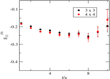
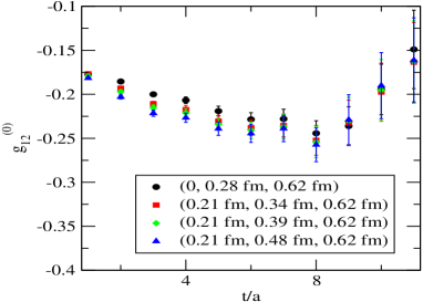
Figure 1: Dependence of bare $g_{12}$ on the size of the GEVP (left) and on the radius of wave functions (right) for the CLS ensemble E5.

Moreover, as shown in figure 2 both GEVP and sGEVP results are consistent, but with a better behavior at large time in the case of the sGEVP. Therefore, the value of the coupling for each ensemble in Table 2 and in the following, corresponds to the sGEVP only. Inspired by Heavy Meson Chiral Perturbation Theory [25] [26] and due to the fact that our action and correlations functions are $\mathcal{O}(a)$ improved, we tried two fit formulae for the extrapolation to the physical point :

$$g_{12} =C_{0}+a^{2}C_{1}\,,$$ (1)

$$g_{12} =C^{\prime}_{0}+a^{2}C^{\prime}_{1}+m^{2}_{\pi}C^{\prime}_{2}\,.$$ (2)

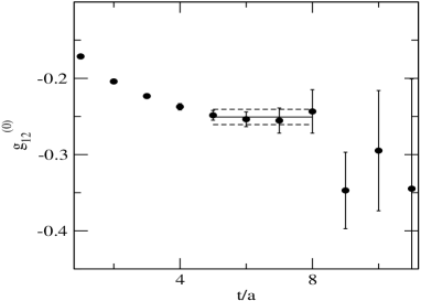
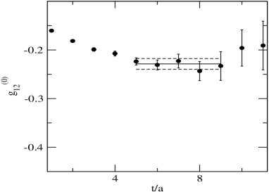
Figure 2: Plateaus of bare $g_{12}$ extracted by GEVP (left) and sGEVP (right) for the CLS ensemble E5.

We show in Figure 3 the continuum and chiral extrapolations. Since the two fits are consistent, we used the result (2) as central value and obtain :

$$g_{12}=-0.17(3)(2)_{\chi}$$

where the first error is statistical and the second originates from the chiral extrapolation and is estimated as the discrepancy between (1) and (2). Fit parameters are collected in Table 2.

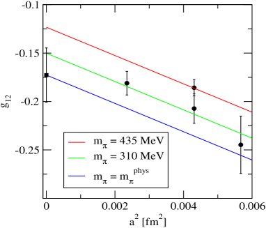
Figure 3: Continuum and chiral extrapolation of $g_{12}$.

Finally, we have to check that we are safe from multi-hadron thresholds due to the emission of pions. The P-wave decay $B^{*^{\prime}}\rightarrow B^{*}(\vec{p})\pi(-\vec{p})$ is kinematically forbidden since $L<3~{}{\rm fm}$. The second, potentially dangerous, decay is the S-wave decay $B^{*^{\prime}}\rightarrow B_{1}^{*}\pi$. But, examining our lattice results for $\Sigma_{12}$, listed in Table 2, we have $230~{}\mathrm{MeV}\leq m_{B^{*^{\prime}}}-m_{B}-m_{\pi}\leq 360~{}\mathrm{MeV}$. Then using recent lattice results [24] with similar lattice spacings : $400~{}\mathrm{MeV}\leq m_{B_{1}^{*}}-m_{B}\leq 500~{}\mathrm{MeV}$, we can conclude that this decay is also forbidden. Finally, as a byproduct of our calculation, we also obtain $g_{11}=0.52(2)$, in excellent agreement with a computation by the ALPHA collaboration focused on that quantity [2], and $g_{22}=0.38(4)$. The continuum and chiral extrapolations for these quantities are shown in Figure 4 while the value of these coupling for each ensemble are listed in Table 2.

	$a\Sigma_{12}$	$g_{12}$	$g_{11}$	$g_{12}$
A5	0.255(8)	-0.245(29)	0.541(5)	0.492(19)
E5	0.222(8)	-0.186(8)	0.535(8)	0.455(10)
F6	0.216(12)	-0.207(15)	0.528(4)	0.474(26)
N6	0.173(7)	-0.181(12)	0.532(6)	0.434(23)

	fit (1)	fit (2)
$C_{0}$	-0.178(29)	-0.155(26)
$C_{1}$	-14.6(7.3)	-9.2(6.6)
$C_{2}$	0.29(16)	-

Table 2: Value of the mass splitting $s\Sigma_{12}$ in lattice units and $g_{12}$ for the different ensembles (left) and fit parameters of eq. (1) and (2) (right).

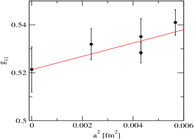
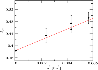
Figure 4: Extrapolation to the continuum and chiral limit of $g_{11}$ and $g_{22}$

6 Conclusion

We have performed a first estimate of the axial form factor $A_{1}(q^{2}_{\mathrm{max}})=g_{12}$ parametrizing the decay $B^{*^{\prime}}\rightarrow B$ at zero recoil and in the static limit of HQET from $N_{f}=2$ lattice simulations. We have obtained a negative value for this form factor. It is almost three times smaller than the $g_{11}$ coupling, but not compatible with zero : $g_{12}=-0.17(4)$ while $g_{11}=0.52(2)$. Moreover we find $g_{22}=0.38(4)$, which is not strongly suppressed with respect to $g_{11}$. Our work is a first hint of confirmation of the statement made in [1] to explain the small value of $g_{D^{*}D\pi}$ computed analytically when compared to experiment.

References

• [1] D. Becirevic, J. Charles, A. LeYaouanc, L. Oliver, O. Pene and J. C. Raynal, JHEP 0301, 009 (2003). [hep-ph/0212177].
• [2] J. Bulava et al. [ALPHA Collaboration], PoS LATTICE 2010, 303 (2010), [arXiv:1011.4393 [hep-lat]]; J. Bulava et al. [ALPHA Collaboration], in preparation.
• [3] D. Becirevic and F. Sanfilippo, [arXiv:1210.5410 [hep-lat]].
• [4] E. Eichten, Nucl. Phys. Proc. Suppl.  4 (1988) 170.
• [5] A. Khodjamirian, R. Ruckl, S. Weinzierl and O. I. Yakovlev, Phys. Lett. B 457, 245 (1999). [hep-ph/9903421].
• [6] J. Bulava, PoS LATTICE 2011, 021 (2011). [arXiv:1112.0212 [hep-lat]].
• [7] T. Burch, C. Gattringer, L. Y. Glozman, C. Hagen, D. Hierl, C. B. Lang and A. Schafer, Phys. Rev. D 74, 014504 (2006). [hep-lat/0604019].
• [8] B. Blossier et al. [ALPHA Collaboration], JHEP 1005, 074 (2010). [arXiv:1004.2661 [hep-lat]].
• [9] D. Mohler and R. M. Woloshyn, Phys. Rev. D 84, 054505 (2011). [arXiv:1103.5506 [hep-lat]].
• [10] M. S. Mahbub et al. [CSSM Lattice Collaboration], Phys. Lett. B 707, 389 (2012). [arXiv:1011.5724 [hep-lat]].
• [11] C. Michael, Nucl. Phys. B 259, 58 (1985)..
• [12] M. Luscher and U. Wolff, Nucl. Phys. B 339, 222 (1990)..
• [13] B. Blossier, M. Della Morte, G. von Hippel, T. Mendes and R. Sommer, JHEP 0904, 094 (2009). [arXiv:0902.1265 [hep-lat]].
• [14] J. Bulava, M. Donnellan and R. Sommer, JHEP 1201, 140 (2012). [arXiv:1108.3774 [hep-lat]].
• [15] A. Hasenfratz and F. Knechtli, Phys. Rev. D 64, 034504 (2001). [hep-lat/0103029];
• [16] M. Della Morte, A. Shindler and R. Sommer, JHEP 0508, 051 (2005). [hep-lat/0506008].
• [17] J. Foley, K. Jimmy Juge, A. O’Cais, M. Peardon, S. M. Ryan and J. -I. Skullerud, Comput. Phys. Commun.  172, 145 (2005). [hep-lat/0505023].
• [18] S. Gusken, U. Low, K. H. Mutter, R. Sommer, A. Patel and K. Schilling, Phys. Lett. B 227, 266 (1989)..
• [19] M. Albanese et al. [APE Collaboration], Phys. Lett. B 192, 163 (1987)..
• [20] B. Blossier, J. Bulava, M. Donnellan and A. Gérardin, Phys. Rev. D 87 (2013) 094518 [arXiv:1304.3363 [hep-lat]].
• [21] P. Fritzsch, F. Knechtli, B. Leder, M. Marinkovic, S. Schaefer, R. Sommer, F. Virotta and R. Sommer et al., Nucl. Phys. B 865 (2012) 397 [arXiv:1205.5380 [hep-lat]].
• [22] M. Della Morte, R. Sommer and S. Takeda, Phys. Lett. B 672, 407 (2009). [arXiv:0807.1120 [hep-lat]].
• [23] P. Fritzsch, F. Knechtli, B. Leder, M. Marinkovic, S. Schaefer, R. Sommer and F. Virotta, Nucl. Phys. B 865, 397 (2012). [arXiv:1205.5380 [hep-lat]].
• [24] C. Michael et al. [ETM Collaboration], JHEP 1008 (2010) 009 [arXiv:1004.4235 [hep-lat]].
• [25] R. Casalbuoni, A. Deandrea, N. Di Bartolomeo, R. Gatto, F. Feruglio and G. Nardulli, Phys. Rept.  281 (1997) 145 [hep-ph/9605342].
• [26] G. Burdman and J. F. Donoghue, Phys. Lett. B 280 (1992) 287.