Lindblad equation approach for the full counting statistics of work and heat in driven quantum systems

Abstract

We formulate the general approach based on the Lindblad equation to calculate the full counting statistics of work and heat produced by driven quantum systems weakly coupled with a Markovian thermal bath. The approach can be applied to a wide class of dissipative quantum systems driven by an arbitrary force protocol. We show the validity of general fluctuation relations and consider several generic examples. The possibilities of using calorimetric measurements to test the presence of coherence and entanglement in the open quantum systems are discussed.

I Introduction

The progress in experimental techniques provides a possibility to study dissipative dynamics of mesoscopic and even quantum systems where fluctuations play a significant roleExperimentBio1 ; ExperimentPendulim ; ExperimentPekola . Unlike for classical systems, the statistics of work is still not well established in the quantum regime. Much attention has been focused on derivations of the quantum versions of fluctuation relations for open quantum systems Campisi ; Campisi1 ; Crooks ; Esposito ; CrooksQuantum ; Mukamel ; Roeck . In particular the fluctuation theorem was derived for an arbitrary open quantum system in Ref.Campisi1 . Despite being a powerful tool, such fluctuation theorems do not provide the detailed information about the statistics of quantum fluctuations which can be of great importance in driven quantum systems. Indeed in quantum optics the sub-Poissonian statistics of photon counts indicates the non-classical states of electromagnetic field MandelWolfBook . Observed first in the atomic resonance fluorescence they have been seen later in many setups including quantum dots, quantum wells and quantum point contactsSubPoissonSources .

Of particular interest is the recent experimental achievement to realize an electrical circuit model of resonance fluorescence in a single artificial atomPashkin . In this setup the atom was represented by a superconducting qubit coupled to a transmission line which can be considered as an effective thermal bath for the open quantum systemCarmichael . In high contrast to the optical devices the electrical circuit can have the temperature compared to the qubit interlevel spacingUstinov2007 so that the work statistics can be strongly modified by thermal fluctuations.

Recently the statistics of finite temperature work fluctuations in a driven single qubit has been treated with the help of a quantum jump method Pekola . In this paper we formulate an alternative approach based on the generalized master equation (GME) which can be applied to a wide class of open quantum systems weakly coupled to the thermal bath. The applicability of the suggested scheme relies on a quite general assumption that the thermal bath is characterized by Markovian dynamics. In this case the open quantum system can be described by the reduced density matrix (DM) which satisfies the Lindblad equation which is a GME with the Lindblad form of the dissipative operator Lindblad . We derive the generating functions which determine the full counting statistics of the work and heat exchange between the quantum system, thermal bath and the classical source which implements an arbitrary drive protocol. Previously the full counting statistics of charge and heat transfer has been extensively investigated in non-equilibrium mesoscopic systemsNazarov ; Kinderman ; Esposito . The present work is dedicated to develop an effective general approach to calculate the fluctuations of work done by the external classical source and the heat exchanged between the quantum system and environment. We demonstrate the difference between the work and heat statistics which becomes especially important for the small exchanged amounts of energy. Several generic examples are considered.

The structure of the paper is as follows. In Sec. II we develop the general formalism of Lindblad equation to calculate the full counting statistics of work and heat in driven quantum systems. In this section we demonstrate that the approximations made in order to trace out the environment variables keep the validity of general fluctuation relations for the quantum work. In Sec.III the heat and work statistics in a single qubit at the finite temperature regime are considered. In Sec. IV we discuss an analytical approach to calculate the long-time statistics of heat in the zero temperature limit. We apply this approach to several generic quantum systems such as a harmonic oscillator, a single qubit and two coupled qubits interacting with separate environments. Conclusions are given in Sec. V.

II Formalism and general fluctuation relations

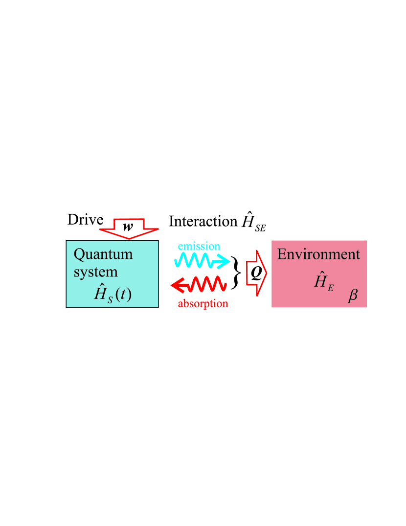
Figure 1: (Color online) Quantum system driven by an external force performing the work $w$. The system interacts with an environment (right) which is at equilibrium with inverse temperature $\beta$. The interaction (middle) is described by an emission and an absorption of energy from the environment. The part of the work transferred to the environment and eventually converted to heat is $Q$.

We consider a system+environment model in which the system is driven and it dissipates energy into an environment as shown schematically in Fig. 1: $\hat{H}(t)=\hat{H}_{S}(t)+\hat{H}_{SE}+\hat{H}_{E}$, where $[\hat{H}_{S}(t),\hat{H}_{E}]=0$. We make a weak coupling approximation and neglect the contribution of the interaction energy $\hat{H}_{SE}$ to the work done by the system. In this case the work $w$ done by the external force is defined according to the two-point projective measurement Work ; Kinderman of the energy $\hat{H}_{S}+\hat{H}_{E}$. The full counting statistics of $w$ is determined by the generating function

$$G_{w}(u,t)={\rm Tr}e^{iu\hat{H}_{S}(t)}\hat{\rho}(t,u),$$ (1)

which depends on the counting field $u$ and measurement time $t$. The DM $\hat{\rho}(t,u)$ is determined by the modified evolution operator

$$\hat{\rho}(t,u)\equiv\hat{U}_{u/2}(t,0)\hat{\rho}(t=0,u)\hat{U}^{\dagger}_{-u/2}(t,0)$$ (2)

$$\hat{U}_{u}(t,0)\equiv e^{iu\hat{H}_{E}}\hat{U}(t,0)e^{-iu\hat{H}_{E}}$$

and the initial condition $\hat{\rho}(t=0,u)=e^{-iu\hat{H}_{S}(0)}\hat{\rho}_{0}$, where $\hat{\rho}_{0}$ is the DM of the system at the moment $t=0$ when we start to count the work. By writing (2) we assume that in the initial state the DM is diagonal in the basis of environment eigenstates $[\hat{H}_{E},\hat{\rho}_{0}]=0$.

The work $w$ should be distinguished from the heat transferred to the thermal bath, $Q$, that has a statistics given by the generating function Campisi ; Esposito

$$G_{Q}(u,t)={\rm Tr}\;\hat{\rho}(t,u).$$ (3)

The DM dynamics is also given by Eqs. (2) but with a different initial state $\hat{\rho}(t=0,u)=\hat{\rho}_{0}$. In general, the work and heat statistics can be drastically different.

Let us take a simple form of the interaction termPuriBook $\hat{H}_{SE}=\hat{S}^{\dagger}\hat{R}+c.c.$ and use the standard Born-Markov approximation assuming that the dynamics of the environment variable $\hat{R}$ is much faster than that of the system variable $\hat{S}$. In this case it is possible to trace out the $\hat{R}$ variables to obtain the reduced DM of the quantum system $\hat{\tilde{\rho}}={\rm Tr}_{R}\hat{\rho}$, which now determines the work generating functions (1,3). Below we omit the tilde implying that DM is a reduced one. The reduced DM satisfies a Lindblad equation which depends on the system variables only Esposito

$$\dot{\hat{\rho}}=\check{A}_{u}[\hat{\rho}],$$ (4)

where $\check{A}_{u}[\hat{\rho}]=-i[\hat{H}_{S},\hat{\rho}]+\check{L}_{u}[\hat{\rho}]$ is a Liouvillian superoperator and $\check{L}_{u}[\hat{\rho}]$ is a time-independent Lindblad dissipative superoperator which describes the interaction of the system with an environmentremark1

$$\check{L}_{u}[\hat{\rho}]=\sum_{j}\Gamma_{-}e^{iu\nu_{j}}\hat{S}_{j}\hat{\rho}\hat{S}^{\dagger}_{j}+\Gamma_{+}e^{-iu\nu_{j}}\hat{S}^{\dagger}_{j}\hat{\rho}\hat{S}_{j}-$$ (5)

$$\Gamma_{-}\{\hat{S}^{\dagger}_{j}\hat{S}_{j},\hat{\rho}\}-\Gamma_{+}\{\hat{S}_{j}\hat{S}^{\dagger}_{j},\hat{\rho}\}.$$

Here $\hat{S}_{j}(\hat{S}^{\dagger}_{j})$ are lowering (rising) operators corresponding to the interlevel spacing $\nu_{j}$, $\{,\}$ is an anti-commutator, and emission and absorption rates satisfy the detailed balance condition $\Gamma_{+}=e^{-\beta\nu_{j}}\Gamma_{-}$. By writing (5) we assume that the driving term is small enough to neglect the perturbation of level spacings $\nu_{j}$. In the opposite case the suggested approach can be modified to express the dissipative operator in the Floquet state representationFloquet . Such approach allows describing Landau-Zehner processes in the dissipative systemsPekolaLZ but this issue is beyond the scope of the present paper.

The general fluctuation relations can be obtained directly from Eqs. (1,4,5). Let us consider a detailed Crooks fluctuation relationCrooks

$$P(w)/P^{tr}(-w)=e^{\beta w},$$ (6)

which relates the probabilities of work $w$ and $-w$ done during forward and time-reversed driving protocols. The work distribution in time-reversed process is determined by the generating function introduced analogously to Eq. (1)

$$G^{tr}_{w}(u,t)={\rm Tr}\;e^{iu\hat{H}_{S}(0)}\hat{\rho}^{tr}(t,u).$$ (7)

Indeed, the evolution of DM $\hat{\rho}^{tr}(t_{1},u)$ when $t_{1}$ runs from $t$ to $0$ is determined by Eqs. (4,5) where $\check{A}^{tr}_{u}[\hat{\rho}]=i[\hat{H}_{S},\hat{\rho}]+\check{L}_{u}[\hat{\rho}]$. The initial condition is $\hat{\rho}^{tr}(t_{1}=t,u)=e^{-iu\hat{H}_{S}(t)}\hat{\rho}_{0}(t)$. The Lindblad superoperator in Eq. (4) is the same for the forward and time-reversed protocols. To satisfy (6) it is enough to demonstrate the generic symmetry relation

$$G_{w}(u,t)=G^{tr}_{w}(i\beta-u,t)$$ (8)

which holds provided that $\hat{H}_{S}(0)=\hat{H}_{S}(t)$ and the initial state for both the forward and time-reversed protocols is the equilibrium one $\hat{\rho}_{0}(t)=\hat{\rho}_{0}(0)=e^{-\beta\hat{H}_{S}(0)}/{\rm Tr}e^{-\beta\hat{H}_{S}(0)}$. The relation (8) follows directly from Eq. (5) since due to the detailed balance and permutation invariance of the trace the Lindblad superoperator (5) satisfies

$${\rm Tr}\;\hat{\rho}_{1}\check{L}_{i\beta-u}[\hat{\rho}_{2}]={\rm Tr}\;\check{L}_{u}[\hat{\rho}_{1}]\hat{\rho}_{2}.$$ (9)

Taking into account that ${\rm Tr}\;\hat{\rho}_{1}[H_{S},\rho_{2}]=-{\rm Tr}\;[H_{S},\rho_{1}]\hat{\rho}_{2}$ we get the relation for the Liouvillians of forward and time-reversed evolutions

$${\rm Tr}\;\hat{\rho}_{1}\check{A}_{u}[\hat{\rho}_{2}]={\rm Tr}\;\check{A}^{tr}_{i\beta-u}[\hat{\rho}_{1}]\hat{\rho}_{2}$$ (10)

and consequently

$${\rm Tr}\;\hat{\rho}_{1}{\rm T}e^{\int_{0}^{t}A_{u}(t_{1})dt_{1}}[\hat{\rho}_{2}]={\rm Tr}\;{\rm\tilde{T}}e^{\int_{0}^{t}A^{tr}_{u}(t_{1})dt_{1}}[\hat{\rho}_{1}]\hat{\rho}_{2}$$ (11)

where ${\rm T}$ and ${\rm\tilde{T}}$ are forward and time-reversed orderings.

Using the formal solutions of Eq.(4) the generating functions can be written as follows

$$G_{w}(u,t)={\rm Tr}e^{iu\hat{H}_{S}(t)}{\rm T}e^{\int_{0}^{t}A_{u}(t_{1})dt_{1}}e^{-iu\hat{H}_{S}(0)}\hat{\rho}_{0}(0)$$ (12)

$$G^{tr}_{w}(u,t)={\rm Tr}\;e^{iu\hat{H}_{S}(0)}{\rm\tilde{T}}e^{\int_{0}^{t}A^{tr}_{u}(t_{1})dt_{1}}e^{-iu\hat{H}_{S}(t)}\hat{\rho}_{0}(t).$$ (13)

Let us assume that both the forward and time-reversed evolution start from equilibrium and moreover $H_{S}(0)=H_{S}(t)=H_{S0}$ so that $\hat{\rho}_{0}(\tau)=e^{-\beta\hat{H}_{S0}}/{\rm Tre^{-\beta\hat{H}_{S0}}}$ for $\tau=0,t$. Then the generic symmetry relation between generating functions (8) immediately follows from Eqs. (12, 13) and the relation (11).

Since the heat $Q$ can be in practice measured either calorimetrically ExperimentPekola or by photon detection, statistics of both $w$ and $Q$ are in general of interest. In certain limits the two statistics approach each other, for example when the energy transfer to the environment is large, or in certain low-temperature measurement protocols. As $Q$ is not generically associated with fluctuation relations such as Eqs. (6), they may fail to apply even if the statistics otherwise approach each other (see Appendix A for discussion). In general it has been shown that the average of the exponentiated heat depends on the details of the driving protocolTalkner . In Appendix B we calculate this quantity explicitly for a single qubit case and demonstrate that it depends on the time of heat statistics measurement.

III Statistics of work and heat in a single qubit

Applying the general approach formulated above we study energy fluctuations in a driven two-level system described by the Hamiltonian

$$H_{S}(t)=\frac{\nu}{2}\hat{\sigma}_{z}+\Omega\cos(\omega_{d}t)\hat{\sigma}_{x},$$ (14)

where $\nu$ is a qubit level spacing and $\Omega$ is a pumping intensity. The dissipation is described by the Lindblad operator (5) with $\hat{S}=(\hat{\sigma}_{x}-i\hat{\sigma}_{y})/2$. To calculate the statistics of energy fluctuations we find the generating functions (1,3) by solving GME (4) numerically assuming that the system was in thermal equilibrium at $t=0$.

As noted in Ref. Pekola the ratio of the first two moments of work satisfies the linear relation

$$\langle\Delta w^{2}\rangle/\langle w\rangle=\nu\coth(\nu/2T)$$ (15)

in the $\langle w\rangle\rightarrow 0$ limit realized for small measuring times. This relation follows from (6) if one assumes that only the probabilities $P(w=-\nu,0,\nu)$ have considerable values. At larger times the significant deviations from Eq.(15) were found Pekola . With our approach we are able to consider the evolution of work statistics at longer times in order to reveal the physical origin of such behavior. We choose the Hamiltonian parameters (14) as $\Omega=0.05\nu$, $\Gamma_{-}=0.007\nu$ and the temperature $\beta=2/\nu$. Starting from the equilibrium state at $t=0$ we plot in Fig.2a the time dependance of the ratios $F_{w}=\tanh(\beta\nu/2)\langle\Delta w^{2}\rangle/(\nu\langle w\rangle)$ and $F_{Q}=\tanh(\beta\nu/2)\langle\Delta Q^{2}\rangle/(\nu\langle Q\rangle)$. For comparison we plot by solid red line the ground state population of the qubit $n_{g}(t)$ which oscillates with a Rabi frequency $\Omega$. The time dependence of $F_{w}(t)$ follows the Rabi oscillations of $n_{g}(t)$. On the other hand the same dependence for the heat statistics $F_{Q}(t)$ has phase-shifted oscillations with respect to $n_{g}(t)$. Moreover in contrast to the work statistics we obtain that the ratio $F_{Q}(t)$ diverges at $t\rightarrow 0$ due to the fluctuating energy exchange between the system and the thermal bath which exists even in the absence of the drive. In this case the dispersion $\langle\Delta Q^{2}\rangle$ stays finite while $\langle Q\rangle=0$.

More generally we obtain that the work distribution e.g. shown in Fig.2b obeys Jarzynski fluctuation relationJarzynski2007 $\langle e^{-\beta w}\rangle=1$ and a particular form of Crooks fluctuation relation $P(w)/P(-w)=e^{\beta w}$ where $P(-w)=P^{tr}(-w)$ since the forward and inverse driving protocols for Eq.(2) coincide. On the other hand the heat distribution shown in Fig.2c does not obey the fluctuation relations and hence the linear relation (15). At elevated temperatures $\beta\ll 1/\nu$ the Rabi oscillations of both the ground state population and the moment ratios $F_{w,Q}(t)$ are strongly suppressed. In this limit we obtain $F_{w}(t)=1$ at arbitrary times as well as $F_{Q}(t)=1$ at $t\gg\Gamma^{-1}_{-},\Omega^{-1}$.

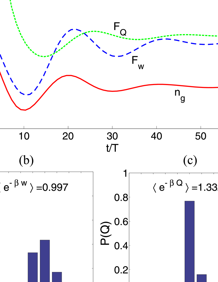
Figure 2: (Color online) (a) The ratio of the two lowest moments of work $F_{w}(t)$ and heat $F_{Q}(t)$ as functions of the measuring time normalized by the period $T=2\pi/\nu$. For comparison, the solid red line shows the Rabi oscillations of the ground state population. All dependencies are averaged over the period $T$. The temperature is $\beta=2/\nu$. (b,c) Distributions of work $w$ and heat $Q$ at the time moment $t=5T$. The calculated probabilities are $P_{w}(-2\nu:3\nu)=[0.0031,0.0589,0.3305,0.4351,0.1693,0.0030]$ and $P_{Q}(-2\nu:2\nu)=[0.0017,0.0609,0.7676,0.1593,0.0106]$. With numerical accuracy determined by the size of the counting field grid the work distribution satisfies Crooks and Jarzynski fluctuation relations. The panel (c) demonstrates lack of the fluctuation relations for the heat.

IV Long-time statistics of heat in driven quantum systems

Our approach based on the Lindblad equation allows analytical calculation of the long-term heat statistics in the quantum limit $\beta\nu\gg 1$. In such regime we completely neglect the absorption events, assuming $\Gamma_{+}=0$ and $\Gamma_{-}=\Gamma$ in (5) so that

$$\check{L}_{u}[\hat{\rho}]=\Gamma e^{iu\nu}\hat{S}\hat{\rho}\hat{S}^{\dagger}-\Gamma\{\hat{S}^{\dagger}\hat{S},\hat{\rho}\}.$$ (16)

For the single interlevel spacing $\nu$ the heat transfer to the environment is proportional to the number of emitted photons in close analogy with quantum optics systems. In this sense the suggested approach can be employed to calculate the steady state statistics of photon counts without solving the non-stationary ME which in general is rather complicated even in the simplest case of a single qubit (two-level atom)MandelWolfBook .

In the steady state regime the statistics of work and heat coincide. In the long-time limit the amount of heat transferred to the environment is much larger than the internal energy of the quantum system. The latter thus can be neglected from Eq. (1) and therefore we get that $G_{w}=G_{Q}$.

In the steady state we calculate the moments of heat distribution measured over a large time interval $t\gg\Gamma^{-1},\Omega^{-1}$. In such a limit the generating function (3) is determined by the Liouvillian eigenvalue $\lambda(u)$ having the largest real part because an asymptotical solution of the GME at $t\rightarrow\infty$ has the form $\rho(u,t)\sim e^{t\lambda(u)}$. Hence the Taylor expansion

$$\lambda(u)=-i\lambda_{1}u-\lambda_{2}u^{2}/2$$ (17)

determines the leading order Gaussian distribution of $Q$ with the moments given by $\langle Q\rangle=\lambda_{1}t$ and $\langle(\Delta Q)^{2}\rangle=\lambda_{2}t$. In order to find the coefficients $\lambda_{1,2}$ in the general case we use an iterative algorithm described in the Sec.IV.2. We start however with calculating the steady state heat fluctuations in a periodically driven harmonic oscillator. Recently the stochastic behavior of damped harmonic oscillator was studied with the help of the quantum trajectoriesHarmonicOscillator . Here we find exactly the eigenvalue $\lambda(u)$ and hence the full counting heat statistics.

IV.1 Harmonic oscillator

Let us consider the following Hamiltonian

$$\hat{H}_{S}=\nu\hat{a}^{\dagger}\hat{a}+\Omega(\hat{a}^{\dagger}e^{-i\omega_{d}t}+\hat{a}e^{i\omega_{d}t}),$$ (18)

where $\hat{a}^{\dagger},\hat{a}$ are creation and annihilation operators and $\Omega$ is the drive force amplitude. The jump operators are $\hat{S},\hat{S}^{\dagger}=\hat{a},\hat{a}^{\dagger}$. In this case the ME has an exact steady state solution $\hat{\rho}_{ho}(t,u)=e^{\lambda(u)t}\hat{D}^{\dagger}(\alpha)|0\rangle\langle 0|\hat{D}(\alpha)$, where $\lambda(u)=\Gamma|\alpha|^{2}(e^{iu\nu}-1)$ and $\hat{D}(\alpha)=\exp(\alpha\hat{a}^{\dagger}-\alpha^{*}\hat{a})$ is a displacement transform with $\alpha=2i\Omega e^{-i\omega_{d}t}/[\Gamma+2i(\nu-\omega_{d})]$. Using $\hat{\rho}_{ho}(t,u)$ to calculate the generating function $G_{Q}(u,t)$ we obtain a Poissonian distribution $P(n)=x^{n}e^{-x}/n!$ of quantized heat $Q=n\nu$, where $x=\Gamma|\alpha|^{2}t$.

The obtained result is consistent with the well known one that a classical current source emits a coherent state of cavity modes which has a Poissonian distribution of photons Glauber . In this model case each event of the heat transfer to the environment occurs at completely random times without any correlation with the previous ones. The linear response relation (15) is satisfied exactly for arbitrary values of dissipation $\Gamma$ and pumping $\Omega$.

IV.2 Single qubit

A generic example which demonstrates significant deviations from linear response relation (15) is a periodically driven single qubit (two- level atom) where quantum correlations between subsequent photon emission events become important MandelWolfBook . The Hamiltonian of such a system (14) can be simplified in rotating wave approximation (RWA) to PuriBook $\hat{H}_{S}=(\Omega\hat{\sigma}_{x}+\delta\hat{\sigma}_{z})/2,$ where we introduce the detuning from resonance $\delta=\nu-\omega_{d}$ and drive intensity $\Omega$. The dissipation is described by the Lindblad operator (16) with $\hat{S}=(\hat{\sigma}_{x}-i\hat{\sigma}_{y})/2$.

The analytical expression of the full counting work statistics in a single qubit is not known. It is possible however to develop a general iterative approach to calculate moments of work distribution measured over a large time interval $t\gg\Gamma^{-1},\Omega^{-1}$. As we discuss above in such a limit the statistics is determined by the Taylor expansion (17) of the Liouvillian eigenvalue $\lambda(u)$ having the largest real part. Note that the zeroth order term in $u$ is absent in (17) due to the existence of a stationary solution at $u=0$ satisfying $\check{A}_{0}[\hat{\rho}^{st}]=0$. In order to find Taylor coefficient $\lambda_{1,2}$ let us consider the expansion of the Liouvillian matrix $\check{A}_{u}$ up to the second order term $\check{A}_{u}[\hat{\rho}]=\check{A}_{0}[\hat{\rho}]+\Gamma[iu\nu-(u\nu)^{2}/2]\hat{S}\hat{\rho}\hat{S}^{\dagger}$ and search for the solution of the eigenvalue problem

$$\check{A}_{u}[\hat{\rho}]=\lambda(u)\hat{\rho}$$ (19)

in the form of an expansion $\hat{\rho}=\hat{\rho}^{st}+\hat{\rho}^{(1)}u+\hat{\rho}^{(2)}u^{2}$. At first we retain the terms linear in $u$. We note that the transposed Liouvillian has one-dimensional kernel $\check{A}^{T}_{0}[\hat{\rho}^{st}_{T}]=0$, where $\hat{\rho}^{st}_{T}=\hat{\sigma}_{0}$ is just an identity matrix. This property holds in general for trace preserving superoperators. We take an inner product with $\hat{\rho}^{st}_{T}$ of both sides in Eq.(19) to obtain the solvability condition which gives the value of $\lambda_{1}$. Substituting the obtained $\lambda_{1}$ to Eq. (19) again we find the correction to the DM $\hat{\rho}^{(1)}$. Next to determine $\lambda_{2}$ we include the terms $\sim u^{2}$ and repeat the above procedure using the known values of the first order corrections.

The heat transfer to the environment occurs via the emission of monochromatic photons $Q=n\nu$, where $n$ is integer. Therefore the heat statistics can be characterized by the Fano factor of photon counts $F_{ph}=\sigma_{Q}^{2}/(\nu\langle Q\rangle)=\lambda_{2}/(\nu\lambda_{1})$. It determines the regimes of sub-Poissonian $F_{ph}<1$ and super-Poissonian $F_{ph}>1$ quantum fluctuations. From the iteration scheme suggested above to calculate $\lambda_{1,2}$ we get the Fano factor for a single qubit $F_{ph}=1-2\Omega^{2}(3\Gamma^{2}-4\delta^{2})/(\Gamma^{2}+2\Omega^{2}+4\delta^{2})^{2}$, which corresponds to the sub-Poissonian regime for small detuning $\delta<\sqrt{3}\Gamma/2$ and otherwise to the super-Poissonian one. This result agrees with the statistics of photon counts in the resonance fluorescence of a two-level atom where the non-classical sub-Poissonian statistics originates from photon antibunching Mandel ; MandelWolfBook ; Cook .

IV.3 Super-Poissonian heat fluctuations and entanglement of two coupled qubits

As discussed above the dependencies shown in Fig.(2) clearly demonstrate that the peculiarities of heat and work statistics can be considered as a signature of the finite coherence in the open quantum system. To obtain more evidence of that we proceed to investigate whether such a purely quantum property as the entanglement between two coupled qubits can be tested by measuring the heat produced by the quantum system.

It is well known that the entanglement between qubits can be induced by dissipative processesEntanglementEnvironment ; Sorin . The photon statistics in this system with incoherent pumping was considered in Ref. delValle, . The conclusion in that case is that the photon statistics is always sub-Poissonian regardless of entanglement. Here we demonstrate that for the case of coherent pumping the statistics of heat transferred to the environment has distinctive features in a subset of the possible entangled states. In general, however, we note that there is no exact correspondence between the statistics of emitted noise and the presence of steady state entanglement in the quantum system. Even a monochromatically driven single qubit can emit both super- and sub-Poissonian distribution of photons Cook . Indeed, two-time correlation functions, such as those for the work or heat statistics, are not solely a property of the steady state density matrix, but are determined also by the transient dynamics of the quantum system between subsequent emission events. However, when consideration is restricted to Hamiltonians of a particular form, such as the setup discussed below, correspondence can arise.

We consider the Hamiltonian of two coupled identical two-level systems which can model the system of inductively coupled phase qubitsCoupledQubits . For simplicity we focus on the quantum fluctuations of $Q$ in the zero temperature limit neglecting the absorption events in (5) completely. Hence this system can be considered as a model of coupled atoms. Its RWA Hamiltonian in case of resonant driving has the form

$$\hat{H}_{S}=\frac{1}{2}\sum_{j=1,2}\Omega\hat{\sigma}^{(j)}_{x}+\omega_{xx}\left(\hat{\sigma}^{(1)}_{x}\hat{\sigma}^{(2)}_{x}+\hat{\sigma}^{(1)}_{y}\hat{\sigma}^{(2)}_{y}\right).$$ (20)

where $\omega_{xx}$ is the qubit coupling and $\Omega$ is a pumping intensity. The parameters of the qubits are assumed to be identical. The dissipation is described by the ME (4) with a Lindblad operator (5) with $\hat{S}_{j}=(\hat{\sigma}^{(j)}_{x}-i\hat{\sigma}^{(j)}_{y})/2$. This form of the dissipation operator corresponds to the qubits interacting with separate thermal baths. The steady state entanglement in this system generated by the interaction with dissipative environment was discussed in Ref. Sorin .

To describe the statistics of work done by each qubit in separate we introduce the generating function which depends on two quantum fields $G_{Q}=G_{Q}(u_{1},u_{2},t)$. By setting $u_{1}=u_{2}$ we obtain the statistics in the double channel which does not distinguish between the heat produced by each of the qubits. The single channel generating function e.g. for the first qubit is given by $G_{Q1}(u_{1},t)=G_{Q}(u_{1},0,t)$.

For further calculations we use the stationary solution of GME given by the kernel of the Liouvillian superoperator $\check{A}_{0}[\hat{\rho}^{st}]=0$ obtained in Ref. Sorin . To find the moments of work we calculate the coefficients in the expansion of the eigenvalue (19)

$$\lambda(u_{1},u_{2})=-i\lambda_{1}(u_{1}+u_{2})-\frac{\lambda_{2}}{2}(u_{1}^{2}+u_{2}^{2})-\lambda_{12}u_{1}u_{2}.$$ (21)

By using the same iterative algorithm as for the single qubit we find an analytical expression for the Fano factor $F_{ph}=\sigma^{2}_{Q}/(\nu\langle Q\rangle)$ which is too long to be written here. In Fig.3a we plot $F_{ph}$ as a function of parameters $\omega_{xx},\Omega$ at fixed $\Gamma=1$. There is a region on this plane, where $F_{ph}>1$ indicating super-Poissonian statistics. The possibility of a super-Poissonian regime is explained by the positive correlation between works extracted from two qubits (see below). It is realized for a strong coupling between the qubits and small dissipation $\omega_{xx}\gg\Omega\gg\Gamma$ and describes bunching of emitted photons which is in contrast to the antibunching in a single qubit resonant fluorescence.

On the qualitative level the photon bunching and super-Poissonian statistics result from the steady state entanglement between the coupled qubitsSorin . Let us transform the steady state DM to the energy basis of the effective Hamiltonian (20). For $\omega_{xx}\gg\Omega$ the energies are given by $\varepsilon_{1}=0$, $\varepsilon_{2,3}=[\omega_{xx}\mp\sqrt{4\Omega^{2}+\omega_{xx}^{2}}]/2$, $\varepsilon_{4}=-\omega_{xx}$. In the regime $\omega_{xx}\gg\Omega$ the basis is formed by the Bell states. In particular $\Phi^{\pm}=|0\rangle_{1}|0\rangle_{2}\pm|1\rangle_{1}|1\rangle_{2}$ correspond to the first two levels separated by the smallest Rabi frequency $\Omega_{R}=\varepsilon_{1}-\varepsilon_{2}\approx\Omega^{2}/\omega_{xx}$. In the DM we neglect the small terms proportional to $\Omega/\omega_{xx}$ and get the following non-zero elements:

$$\rho_{11}=\rho_{22}=1/2-\Omega_{R}^{2}/4X,\;$$ (22)

$$\rho_{12}=\rho^{*}_{21}=[\Gamma^{2}-i\Gamma\Omega_{R}]/2X,$$

where $X=\Omega_{R}^{2}+\Gamma^{2}$ and $\rho_{33}=\rho_{44}=1/2-\rho_{11}$. Hence at $\Gamma\gg\Omega_{R}$ the most populated are the Bell states $\Phi^{\pm}$.

In this case the emission of a photon by one of the qubits can be considered as a projective measurement Pekola which drives the other qubit to the excited state and hence triggers an emission of the next photon once this qubit relaxes. In Fig.3a we plot by a white solid line the boundary $\omega_{xx}=\Omega^{2}/2\Gamma$ which separates the region with finite steady state entanglement $\omega_{xx}>\Omega^{2}/2\Gamma$ from that of non-entangles statesSorin . The super-Poisson statistics of work is realized only for the entangled states and can be considered as a possible experimental signature of entanglement.

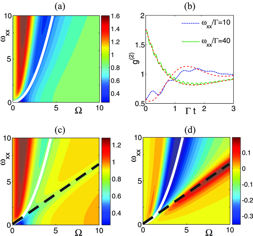
Figure 3: (Color online) Statistics of heat produced by two coupled qubits. (a) Fano factor in a double channel $F_{ph}=\sigma_{Q}^{2}/(\nu\langle Q\rangle)$ as a function of interaction strength $\omega_{xx}$ and pumping $\Omega$. (b) Second order correlation functions - the probabilities of sequential photon emission by the two-qubit system compared to the effective three level approximation model (dashed curves). The parameters are $\Omega=5$, $\Gamma=1$ and $\omega_{xx}=10$ (solid curve), $\omega_{xx}=40$ (dotted curve). (c) Correlation function $C_{12}/(\nu^{2}\Gamma t)$ of heat produced by each of the qubits in separate. (d) Fano factor of heat released by one of the qubits $F_{ph1}=2\sigma_{Q1}^{2}/(\nu\langle Q\rangle)$. The white solid curves show the boundary between the steady state entangled and non-entangled regimes. The relaxation rate is $\Gamma=1$. The super-Poissonian regimes both in the double and the single channels correspond to finite entanglement. Dashed black line (b,c) shows the resonance condition $\Omega=\sqrt{2}\omega_{xx}$.

To obtain a quantitative description of the photon bunching we consider the second order correlation function of photon emission intensityMandelWolfBook $g^{(2)}(t)$ plotted in Fig.3d for the parameters $\Omega/\Gamma=5$ and $\omega_{xx}/\Gamma=10$ (blue dotted curve) and $\omega_{xx}/\Gamma=40$ (green solid curve). It demonstrates the photon bunching $g^{(2)}(0)\geq g^{(2)}(t)$ at large values of $\omega_{xx}\gg\Omega\gg\Gamma$. The correlator has rapid oscillations with a frequency determined by the coupling $\omega_{xx}$ superimposed over the smooth behavior.

In order to get more insight in the details of the curves shown in Fig.(3)b we obtain an analytical description of the correlations averaged over the fast oscillations neglecting the small elements of the DM proportional to $\Omega/\omega_{xx}$ and $\Gamma/\omega_{xx}$. This approximation results in an effective three-level ansatz for the DM with non-zero elements $\tilde{\rho}_{ij}=\rho_{ij}$ for $i,j=1,2$ and $\tilde{\rho}_{33}=\rho_{33}+\rho_{44}$. The steady state is determined by (22). The resulting ME has a Hamiltonian with non-zero matrix elements $H_{11}=-\Omega_{R}/2$ and $H_{22}=\Omega_{R}/2$. The elements $H_{33},H_{44}$ drop from the ME for the above ansatz of DM. The Lindblad superoperator (16) has $\hat{S}=\hat{S}_{3}$ which is a $3\times 3$ matrix with non-zero elements $(\hat{S}_{3})_{13}=(\hat{S}_{3})_{23}=i\sqrt{\Gamma/2}$ and $(\hat{S}_{3})_{31}=-(\hat{S}_{3})_{32}=i\sqrt{\Gamma}$. The second order correlator $\langle g^{(2)}\rangle(t)=\langle\hat{S}_{3}^{\dagger}\hat{S}_{3}^{\dagger}(t)\hat{S}_{3}(t)\hat{S}_{3}\rangle/\langle\hat{S}_{3}^{\dagger}\hat{S}_{3}\rangle^{2}$ gives the correlator $g^{(2)}(t)$ of the full system averaged over the period of fast oscillations $\omega^{-1}_{xx}$ . Most importantly the operator $\hat{S}_{3}$ allows for the two simultaneous quantum jumps from the steady state by (22) since $\hat{S}^{2}_{3}\hat{\rho}^{st}\hat{S}^{{}^{\dagger}2}_{3}\neq 0$. In this model the two photons can be emitted simultaneously which gives the finite value of $g^{(2)}(t=0)$.

It is possible to find $\langle g^{(2)}\rangle(t)$ analytically by solving the ME with $u=0$ and the initial state after the first quantum jump given by $\hat{S}_{3}\hat{\rho}^{st}\hat{S}^{\dagger}_{3}$. Indeed from the three-level ME we see that the equations for the components $\tilde{\rho}_{11}$ and $\tilde{\rho}_{22}$ coincide and thus we can reduce the problem to the second order ME. It can be solved with arbitrary initial conditions yielding the correlator

$$\langle g^{(2)}\rangle(t)=1+e^{-\Gamma t}\left[\frac{(x^{2}-1)}{2}\cos(\Omega_{R}t)-x\sin(\Omega_{R}t)\right],$$ (23)

where we introduce $x=\Gamma/\Omega_{R}$. The function $\langle g^{(2)}\rangle(t)$ is plotted in Fig. (3)b by dashed lines. It has a damped oscillating behavior determined by the competition of an effective Rabi frequency $\Omega_{R}$ and the damping $\Gamma$. In high contrast to the single qubit case the two-point correlation function can have a maximum at $t=0$ at large values of $\omega_{xx}$ which corresponds to the bunching of photons produced by the entangled states of the two qubit system.

Next we use the expansion (21) to find the correlation function of heat produced by each of the qubits

$$C_{12}=\langle Q_{1}Q_{2}\rangle-\langle Q_{1}\rangle\langle Q_{2}\rangle=\lambda_{12}t.$$ (24)

In Fig. 3(c) one can see two peaks of $C_{12}$ as a function of parameters $\Omega,\omega_{xx}$. One of them corresponds to non-zero entanglement between the qubits and produces super-Poisson statistics of work. The second peak is located at $\omega_{xx}=\Omega/\sqrt{2}$ as indicated by the dotted black line in Fig. 3(c). For such parameters the spectrum of effective RWA Hamiltonian (20) is degenerate since the two levels coincide, $\varepsilon_{2}=\varepsilon_{4}$. The subspace of eigenstates for this level is given by $\psi_{24}=c_{2}\psi_{2}+c_{4}\psi_{4}$, where $c_{2,4}$ are arbitrary coefficients, and the orthogonal basis functions are $\psi_{2}=(\sqrt{2},1,1,\sqrt{2})/\sqrt{6}$ and $\psi_{4}=(0,-1,1,0)/\sqrt{2}$. To understand the nature of positive correlation $C_{12}$, let us consider the case of small relaxation $\Omega,\omega_{xx}\gg\Gamma$ when the DM is diagonal $\hat{\rho}=\left(|11\rangle\langle 11|+|00\rangle\langle 00|+|01\rangle\langle 01|+|00\rangle\langle 00|\right)/4$ . After the photon emission for example, by the first qubit the DM is projected to $\hat{\rho}=\hat{S}_{1}\hat{\rho}_{0}\hat{S}^{\dagger}_{1}=(|01\rangle\langle 01|+|00\rangle\langle 00|)/4$ because the first qubit is bound to be in the ground state. Taking the time average of the DM we find that during the subsequent evolution the first term produces a contribution $|01\rangle\langle 01|\rightarrow|\psi_{24}\rangle\langle\psi_{24}|$ with $c_{2}=1/\sqrt{6}$ and $c_{4}=1/\sqrt{2}$ so that in this case the amplitude of $\psi_{24}$ is asymmetric. At the same time the second term $|00\rangle\langle 00|$ evolves into a symmetric time-averaged population of the qubits. That is the probability for the second qubit to be in the excited state and hence to emit a photon is larger than for the first one. Thus the peak of $C_{12}$ is accompanied by the drop of the single channel Fano factor as shown in Fig. 3(d) so that the statistics of work in double channel is sub-Poissonian, $F_{ph}<1$ [Fig. 3(a)].

V Conclusion

To conclude, we have developed a formalism of Lindblad equation to calculate the statistics of energy fluctuations in dissipative quantum systems driven by an external force. We introduced generating functions of work and heat exchanged between the system, the classical driving source and the thermal bath which can be found by solving the Lindblad equation. The general fluctuation relations are shown to be valid for the resulting work statistics. Applying this formalism to the generic examples of a harmonic oscillator, a single and two coupled qubits we have shown that calorimetric measurements of heat statistics can indicate the presence of finite coherence and entanglement in the open quantum systems.

It is our pleasure to thank Prof. Jukka Pekola for discussions. This work was supported by the Academy of Finland, the European Research Council (Grant No. 240362-Heattronics), and the EU-FP 7 INFERNOS (Grant No. 308850) programs.

Appendix A Measuring work statistics at zero temperature

At zero temperature, it is possible to determine the long-time statistics $G_{w}(u,t\to\infty)$ of the total work $w$ by a measurement of the statistics $G_{Q}(u,t\to\infty)$ of the heat dissipated to the environment $Q$. The measurement scheme is to drive the system only during the time interval $0<t<t_{1}$, after which the system Hamiltonian is made constant and to coincide with the initial state, $H_{S}(t)=H_{S}(0)$ for $t>t_{1}$. In this case, the internal energy stored in the system is eventually emitted to the zero-temperature environment, Pekola and one finds $G_{w}(u,t\to\infty)=G_{Q}(u,t\to\infty)$.

This correspondence can be proven directly using our master equation formulation. We start with the observation that for a given constant $u$, we have at time $t>t_{1}$,

$$\lim_{\beta\to\infty}\check{A}_{u}(t)\{P_{0}\}=0\,,$$ (25)

for the ground state density matrix $P_{0}=\lvert{0}\rangle\langle{0}\rvert$. Indeed, $\hat{S}P_{0}=P_{0}\hat{S}^{\dagger}=0$. Therefore, $P_{0}$ is a steady state of the $u$-dependent time evolution for $\beta\to\infty$, and we find for $\beta,t\to\infty$,

$${\cal T}e^{\int_{0}^{t}\mathrm{d}t^{\prime}\,\check{A}_{u}(t^{\prime})}\{P_{0}\}\to f(u,t)P_{0}\,,$$ (26)

where $f(u,t)$ is a scalar function. The initial state for $G_{w}$ is $\rho_{0}=e^{-(iu+\beta)H_{S}(0)}/\operatorname{Tr}[e^{-\beta H_{S}(0)}]\to e^{-iu\epsilon_{0}}P_{0}$ for $\beta\to\infty$, where $\varepsilon_{0}$ is a ground state energy. It then immediately follows that for $\beta,t\to\infty$,

$$G_{w}(u,t)\to e^{-iu\epsilon_{0}}\operatorname{Tr}[e^{iuH_{S}(0)}f(u,t)P_{0}]=f(u,t)\,.$$ (27)

On the other hand, we have for the dissipated work, for $\beta,t\to\infty$,

$$G_{Q}(u,t)=\operatorname{Tr}{\cal T}e^{\int_{0}^{t}\mathrm{d}t^{\prime}\,\check{A}_{u}(t^{\prime})}\{P_{0}\}\to f(u,t)\,.$$ (28)

Therefore, in this measurement scheme we find $G_{w}(u,t\to\infty)=G_{Q}(u,t\to\infty)$, which is also the result one would expect based on physical arguments.

Note that above $u$ is taken as a $\beta$-independent constant while taking the limit $\beta\to\infty$. Therefore, although we find that $G$ converges pointwise to $G_{w}$, this does not imply that the dissipated work satisfies the Jarzynski equality. Indeed, while $G_{w}(i\beta,t)=1$, the result above does not imply that $\lim_{t\to\infty,\beta\to\infty}G_{Q}(i\beta,t)=1$.

Appendix B Lack of fluctuation relations for $Q$

The lack of universal fluctuation relations for the heat $Q$ can be easily demonstrated based on the master equation approach. This can be seen in the model of an non-driven qubit coupled to an environment. The corresponding Liouvillian is

$$\check{A}_{u}(t)\{\rho\} =-i[\frac{\nu}{2}\sigma_{z},\rho]+\Gamma\Bigl{(}e^{iu\nu}\hat{S}\rho\hat{S}^{\dagger}-\frac{1}{2}\{\hat{S}^{\dagger}\hat{S},\rho\}\Bigr{)}$$ (29)

$$+\Gamma e^{-\beta\nu}\Bigl{(}e^{-iu\nu}\hat{S}^{\dagger}\rho\hat{S}-\frac{1}{2}\{\hat{S}\hat{S}^{\dagger},\rho\}\Bigr{)}\,.$$

Solving the time dependence of the $u$-dependent master equation, we find the generating function for the dissipated work

$$G_{Q}(u,t) =\frac{\cos(u\nu)+\cosh(\beta\nu)}{1+\cosh(\beta\nu)}$$ (30)

$$-e^{-(e^{-\beta\nu}+1)\Gamma t}\frac{e^{(\beta-iu)\nu}(e^{iu\nu}-1)^{2}}{(e^{\beta\nu}+1)^{2}}\,.$$

This implies that the heat only obtains values $Q=\pm\nu,\,0$, as can be expected based on the limited internal energy of the qubit.

The above implies that the expectation value $\langle{e^{-\beta Q(t)}}\rangle=G_{Q}(i\beta,t)$ is time dependent. Because this occurs at equilibrium with all Hamiltonians time independent, there can be no fluctuation relation of the form $\langle{e^{-\beta Q(t)}}\rangle=e^{-\beta\Delta F}$ where $\Delta F$ is a difference between two equilibrium free energies. This result is in agreement with the general non-equilibrium equality for the heat derived in Ref. Talkner, .

Moreover, Eq. (30) serves as a simple example for the above discussion of the zero-temperature limit. Indeed, for given fixed $u$ we have $\lim_{\beta,t\to\infty}G_{Q}(u,t)=1=G_{w}(u,t)$. However, at the same time, $\lim_{\beta,t\to\infty}G_{Q}(i\beta,t)=2$.

References

- (1) D. Collin, F. Ritort, C. Jarzynski, S. B. Smith, I. Tinoco, C. Bustamante, Nature 437 231 (2005); J. Liphardt, B. Onoa, S. B. Smith, I. Tinoco and C. Bustamante, Science 292 733 (2001); J. Liphardt, S. Dumont, S. B. Smith, I. Tinoco and C. Bustamante, Science 296 1832 (2002);
- (2) F. Douarche, S. Ciliberto, A. Petrosyan, I. Rabbiosi, Europhys. Lett. 70 593 (2005).
- (3) J.P. Pekola, P. Solinas, A. Shnirman, D.V. Averin, arXiv:1212.5808.
- (4) M. Campisi, P. Hänggi, and P. Talkner, Rev. Mod. Phys. 83, 771 (2011); 83, 1653(E) (2011).
- (5) M. Campisi, P. Talkner, and P. Hänggi, Phys. Rev. Lett. 102, 210401 (2009).
- (6) M. Esposito, U. Harbola, and S. Mukamel, Rev. Mod. Phys. 81, 1665 (2009).
- (7) G. E. Crooks, J. Stat. Mech. P10023, (2008).
- (8) S. Mukamel, Phys. Rev. Lett. 90, 170604 (2003).
- (9) W. De Roeck and C. Maes, Phys. Rev. E 69 026115 (2004).
- (10) G. E. Crooks, Phys. Rev. E 60, 2721 (1999).
- (11) L. Mandel and E. Wolf, Quantum coherence and quantum optics, Cambridge University Press (1995).
- (12) J. Kim, O. Benson, H. Kan, and Y. Yamamoto, Nature 397, 500 (1999); Z. L. Yuan, B. E. Kardynal, R. M. Stevenson, A. J. Shields, C. J. Lobo, K. Cooper, N. S. Beattie, D. A. Ritchie, and M. Pepper, Science 295, 102 (2002).
- (13) O.V. Astafiev, A. M. Zagoskin, A. A. Abdumalikov, Yu.A. Pashkin, T. Yamamoto, K. Inomata, Y. Nakamura, and J. S. Tsai, Science 327, 840 (2010); A. A. Abdumalikov, O.V. Astafiev, Yu.A. Pashkin, Y. Nakamura, and J. S. Tsai, Phys. Rev. Lett. 107, 043604 (2011).
- (14) H.J. Carmichael, Statistical methods in quantum optics 2, Springer-Verlag Berlin Heidelberg (2008).
- (15) J. Lisenfeld, A. Lukashenko, M. Ansmann, J. M. Martinis, and A. V. Ustinov, Phys. Rev. Lett. 99, 170504 (2007).
- (16) F.W. J. Hekking and J. P. Pekola, Phys. Rev. Lett., 111, 093602 (2013).
- (17) A. Kossakowski, Rep. Math. Phys. 3 247 (1972); G. Lindblad, Commun. Math. Phys. 48 119 (1976).
- (18) D. A. Bagrets, Y. V. Nazarov, Phys. Rev. B 67, 085316 (2003).
- (19) M. Kindermann, and S. Pilgram, Phys. Rev. B 69, 155334 (2004).
- (20) P. Talkner, E. Lutz, and P. Hänggi, Phys. Rev. E 75, 050102 (2007);
- (21) R.R. Puri Mathematical Methods of Quantum Optics (Berlin: Springer) 2001.
- (22) The counting factors in Eq.(5) arise from the generalized correlation functions of the environment variables . This approach can be applied to systems with multiple eigenfrequencies . It is valid in case of the weak drive which means that the drive does not change the eigenfrequencies.
- (23) H.-P. Breuer and F. Petruccione, Phys. Rev. A, 55 3101 (1997); M. Grifoni, P. Hänggi, Physics Reports 304, 229 (1998)
- (24) P. Solinas, D. V. Averin, and J. P. Pekola, Phys. Rev. B 87, 060508(R) (2013); S. Gasparinetti, P. Solinas, Y. Yoon, and J. P. Pekola, Phys. Rev. B 86, 060502 (2012).
- (25) P. Talkner, M. Campisi and P. Hanggi, J. Stat. Mech., P02025 (2009)
- (26) C. Jarzynski, C.R. Physique 8, 495 (2007); G.N. Bochkov, Yu. E. Kuzovlev, Phys. Usp. 56 590 (2013).
- (27) J. M. Horowitz, Phys. Rev. E 85, 031110 (2012).
- (28) R.J. Glauber, Phys. Rev., 131 2766 (1963).
- (29) R.J. Cook, Phys. Rev. A, 22, 1078 (1980).
- (30) L. Mandel, Opt. Lett., 4, 205 (1979).
- (31) J. Li and G.S. Paraoanu, New J. Phys. 11, 113020 (2009).
- (32) S. F. Huelga and M. B. Plenio, Phys. Rev. Lett. 98, 170601 (2007);
- (33) E. del Valle, J. Opt. Soc. Am. B 28, 228 (2011) .
- (34) John Clarke, Frank K. Wilhelm, Nature 453, 1031 (2008).