Almost-Killing conserved currents:
a general mass function

Abstract

A new class of conserved currents, describing non-gravitational energy-momentum density, is presented. The proposed currents do not require the existence of a (timelike) Killing vector, and are not restricted to spherically symmetric spacetimes (or similar ones, in which the Kodama vector can be defined). They are based instead on almost-Killing vectors, which could in principle be defined on generic spacetimes. We provide local arguments, based on energy density profiles in highly simplified (stationary, rigidly-rotating) star models, which confirm the physical interest of these almost-Killing currents. A mass function is defined in this way for the spherical case, qualitatively different from the Hernández-Misner mass function. An elliptic equation determining the new mass function is derived for the Tolman-Bondi spherically symmetric dust metrics, including a simple solution for the Oppenheimer-Schneider collapse. The equations for the non-symmetric case are shown to be of a mixed elliptic-hyperbolic nature.

I Introduction

In a previous paper Ruiz et al. (2012), we studied the role of the ergosphere in the Blandford-Znajeck mechanism. The essential tool for to identify jet formation in our numerical simulations was the energy flux density of the electromagnetic field. The spacetime geometry was given by a family of stationary and axisymmetric star models Ansorg et al. (2002, 2003). This allowed us to use the timelike Killing vector for constructing the energy-momentum conserved current of the electromagnetic field. The energy flux density could then be identified in a physically sound way. Extending this approach to dynamical (non stationary) cases is a challenge, because of the lack of a well defined conserved current for generic spacetimes.

Energy conservation is one of the most outstanding physical paradigms. In General Relativity, it can be formulated through the covariant equation

$$\nabla_{b}T^{ab}=0\,,$$ (1)

where the stress-energy tensor contains all forms of energy of non-gravitational origin: it vanishes in vacuum, even if gravitational waves can propagate there. Gravitational energy is not included because in General Relativity gravitation is rather described by the curvature of spacetime. Nevertheless, the gravitational field gets coupled to the matter fields and this coupling does not allow to write down (1) as an integral conservation law. $T^{ab}$ is indeed a two-tensor and the vanishing of its covariant divergence contains source terms in curved spacetimes. Conserved quantities, such as energy and momentum, cannot be properly defined in the standard way (by means of the divergence theorem) because the source terms turn the required integral conservation law into a balance law, with a bulk contribution depending on the (non-covariant) connection coefficients.

A conserved current can be obtained, however, when the spacetime admits a continuous symmetry, associated to some Killing vector field (KV) $\zeta$. In this case, the vector current

$$J^{a}={T^{a}}_{b}\,\zeta^{b}\,,$$ (2)

is conserved, allowing for the Killing equation, that is $\,\nabla_{a}J^{a}=0$. The divergence theorem allows to obtain an integral conservation law. Note that the gravitational field is still coupled to the matter fields, but this coupling is encoded here through the Killing vector $\zeta$. When it is timelike, we can interpret the current (2) as the energy-momentum density current associated to a freely falling observer which is momentarily at rest with respect the stationary fleet of observers. Let us stress that we are still dealing with non-gravitational energy, which we will call for short mass in what follows, as the current (2) vanishes in vacuum.

Note also that the current (2) is not the only one which can be useful in the KV case: the related current

$${R^{a}}_{b}\,\zeta^{b}$$ (3)

is also conserved. Modulo a global factor, which could always be used for rescaling any KV, this alternative conserved current differs from the usual choice (2) by a term proportional to the KV itself, namely

$$\triangle J^{a}=T/2~{}\zeta^{a}\,.$$ (4)

In stationary spacetimes, where $\zeta=\partial_{t}\,$ can be interpreted as representing the co-moving fleet of observers, the difference between (2) and (3) can be understood just as an energy density redefinition, not affecting the energy flux. The results obtained in Ruiz et al. (2012) with the current (2) would not change if we had used (3) instead.

The (non-gravitational) energy density $\mathcal{E}$ and the energy flux density $S^{i}$ can be identified by considering a 3+1 decomposition of the spacetime such that the metric can be written as

$$ds^{2}=-\alpha^{2}~{}dt^{2}+\gamma_{ij}~{}(dx^{i}+\beta^{i}~{}dt)\,(dx^{j}+\beta^{j}~{}dt)\,,$$ (5)

so we get

$$\sqrt{\gamma}\,\mathcal{E}=-\sqrt{-g}\,J^{0}\,,\qquad\sqrt{\gamma}\,\mathcal{S}^{i}=-\sqrt{-g}\,J^{i}\,,$$ (6)

where $\sqrt{\gamma}$ is the space volume element. In adapted coordinates, where the timelike KV of stationary spacetimes can be written as $\zeta^{a}=\delta^{a}_{(t)}$, the differential current (4) would contribute to the resulting energy density but not to the energy-flux density. Note that, although it could be useful in some cases to include the geometrical factor $\sqrt{\gamma}$ into the Energy density definition, we rather prefer to work here with a quantity which is independent of the space coordinates system, namely

$$\mathcal{E}=-n_{a}J^{a}=-\alpha J^{0}\,,$$ (7)

where $n_{a}=\alpha\,\delta_{a}^{(t)}$ stands for the future pointing timelike unit normal (up to a sign, it can be interpreted as the four-velocity of a non-rotating fiducial observer).

The extension of the conserved current (2) to dynamical spacetimes can be done in some special cases. In the spherically symmetric case, the warped structure of the spacetime allows the use of the Kodama vector $K$ as a replacement for the missing KV Kodama (1980). The resulting Kodama current

$$J_{Kodama}^{a}={T^{a}}_{b}\,K^{b}\,,$$ (8)

is still conserved and leads to a definition of mass which allows to recover the Hernández-Misner mass function Hernandez Jr and Misner (1966); Abreu and Visser (2010) (see section III or details). In the vacuum (Schwarzschild) case, the Kodama vector $K$ coincides with the standard KV. Also, in dust-filled spacetimes, the matter current

$$J_{dust}^{a}={T^{a}}_{b}\,u^{b}\,,$$ (9)

is conserved, where $u$ is the four-velocity of the particles.

Unfortunately, these ideas do not work for generic dynamical scenarios, where one has to deal with different types of matter and fields in non-symmetric spacetimes. In these cases, the idea of approximate symmetry, or the almost-Killing vector fields (AKV), could be a starting point to build up conserved currents, which could have then some physical interest. In this paper we propose to consider the almost-Killing current

$$J^{a}_{AK}=\frac{1}{4\pi}\,{R^{a}}_{b}\,\xi^{b}\,,$$ (10)

which is conserved if $\xi$ is an almost-Killing vector field, as we will show in the next section (the $1/4\pi\,$ factor is introduced for further convenience). We provide local arguments, based on the energy density profiles of some simple star models, supporting the choice of the almost-Killing current (46), rather than the standard choice (2), for describing mass conservation in many physical scenarios.

Spherically symmetric metrics are considered in section III, either in the static case (the Schwarzschild constant density star) or in the dynamical one (Tolman-Bondi dust solutions). A mass function can be defined due to the essentially 1D character of the problem. In the static case, we show that it coincides with the standard Hernández-Misner mass function. This is no longer true in the dynamical (dust) case, where we provide a single elliptic-type equation determining the mass-energy function obtained from the AK current $J_{AK}$. The space-homogeneous (Friedmann-Robertson-Walker) case is considered in the Oppenheimer-Snyder collapse scenario. A solution is obtained for the mass function which is qualitatively different from the Hernández-Misner mass. This function may be of interest in studying local density perturbations in a cosmological background.

Non-spherical spacetimes are finally considered in section IV. In the stationary case, more specifically for rigidly-rotating axially-symmetric star models, our results confirm the advantage of taking the almost-Killing current $J^{a}_{AK}$ as the starting point for physical applications. In the generic, non-symmetric case, we write down the full set of equations, which has a mixed elliptic-hyperbolic character. We discuss all these results in the final section.

II Almost-Killing vector fields

Spacetimes with continuous symmetries can be characterized by the fact that they admit non-trivial solutions to the Killing equation (KE), namely

$$\mathcal{L}_{\zeta}\,g_{ab}=\nabla_{a}\zeta_{b}+\nabla_{b}\zeta_{a}=0\,.$$ (11)

Since most astrophysical scenarios do not satisfy the above requirement, there has been a considerable amount of work on constructing intrinsic ways of characterizing almost-symmetric spacetimes. A precise implementation of the concept of almost-symmetry has been provided by Matzner Matzner (1968). Starting from a variational principle, it defines a measure of the symmetry deviation of any given spacetime. This idea has been used by Isaacson to study high frequency gravitational waves in which, by defining a steady coordinate system, the radiation effects can be easily separated from the background metric Isaacson (1968). Zalaletdinov related this symmetry deviation with a measure of the inhomogeneity of the spacetime which can be related with some entropy concept Zalaletdinov (2000). More recently Bona et. al. have shown that harmonic almost-Killing motions provide a convenient generalization of the standard harmonic motions Bona et al. (2005).

Vector fields verifying the almost-Killing equation (AKE)

$$\nabla_{b}\left[\nabla^{a}\xi^{b}+\nabla^{b}\xi^{a}-{\mu}\,(\nabla\cdot\xi)\,g^{ab}\right]=0\,,$$ (12)

with $\mu$ a given constant, provide an interesting generalization of the KV Taubes (1978); Bona et al. (2005). Of course, any solution of KE is also a solution of the AKE. Moreover, as pointed out by York York (1974), any vector field that asymptotically satisfies the KE is, in general, asymptotically a solution of Equation (12). The AKE can be obtained by minimizing, on a fixed background, the Lagrangian density Bona et al. (2005)

$$L=\nabla^{(a}\xi^{b)}\,\nabla_{(a}\xi_{b)}-\frac{\mu}{2}\,(\nabla\cdot\xi)^{2}\,,$$ (13)

which can be interpreted as a generic invariant measure of the deviation from the strict Killing symmetry condition. The parameter $\mu$ measures the relative weight of the two quadratic scalars in the Lagrangian.

Notice that, by commuting the covariant derivatives in (12), the AKE can also be expressed as a generalized wave equation, namely

$$\square\,\xi^{a}+{R^{a}}_{b}\,\xi^{b}+(1-\mu)\,\nabla^{a}(\nabla\cdot\xi)=0\,.$$ (14)

It follows that, for any given spacetime, the initial value problem of the above equation is a standard Cauchy problem in the generic case $\mu\neq 2$ (i.e. a second order partial-differential-equation system for the four vector components). In particular, if $\mu=1$, the principal part of the AKE is harmonic which, in adapted coordinates, implies Bona et al. (2005)

$$g^{bc}\,\partial_{t}\,{\Gamma^{a}}_{bc}=0\,.$$ (15)

In asymptotically flat spacetimes, this condition asymptotically coincides with the so-called minimal distortion shift condition used in numerical relativity to minimize changes in the shape of volume elements of the spacetime during evolution Smarr and York (1978).

Almost-Killing mass function

Allowing for (14), the AKE can be also interpreted as providing an explicit expression for the almost-Killing current $J_{AK}$, associated with the AKV field $\xi$, namely

$$4\pi\,J^{a}_{AK}\equiv{R^{a}}_{b}\,\xi^{b}=\nabla_{b}\nabla^{[a}\xi^{b]}-(1-{\mu}/2)~{}\nabla^{a}(\nabla\cdot\xi)\,.$$ (16)

This current is identically conserved if and only if the divergence of the AKV verifies

$$\Box\,(\nabla\cdot\xi)=0\,,$$ (17)

as it its the case for both KV and homothetic vectors, which are just particular AKE solutions.

If this is not the case, only quasilocal quantities could be obtained from (16), unless we take the parameter choice $\mu=2$ (notice that the value of the parameter $\mu$ is irrelevant if $\xi$ is actually a KV or an homothety). Therefore, in what follows we will take

$$J^{a}_{AK}\equiv\frac{1}{4\pi}~{}{R^{a}}_{b}\,\xi^{b}=\frac{1}{4\pi}~{}\nabla_{b}\nabla^{[a}\xi^{b]}$$ (18)

unless otherwise stated.

The current defined by the right-hand side of (18) is actually the Komar current associated to the vector field $\xi$ Komar (1959); Wald (1984) and, by construction, it is divergence-free. The total mass $M$ contained in a closed space volume $V$ on a constant time slice $\Sigma$ is given by

$$M=\int_{\Sigma}\,\mathcal{E}~{}dV=-\int_{\Sigma}\alpha\sqrt{\gamma}\,J^{0}d^{3}x\,.$$ (19)

Allowing for (18), the above expression can be written as a surface integral by means of the divergence theorem, namely

$$M_{AK}=\frac{1}{4\pi}\int_{\partial\Sigma}\,n_{b}\,\nabla^{[a}\xi^{b]}~{}d\sigma_{a}\,,$$ (20)

where $d\sigma_{b}$ is the oriented area element for the spacelike surface limiting the volume $V$. We have seen how the almost-Killing approach allows to define conserved currents and quasi-local quantities such as $M_{AK}$ in Eq. (20). However, there is an issue of choice. There are infinitely many AK currents, one for every choice of the seed vector field $\xi$. The resulting conserved current represents the energy-momentum density associated to the fleet of observers with worldlines aligned with the selected AKV vector field. A judicious choice of the seed AKV is then required in order to get a physically sound interpretation. If the spacetime admits either a timelike KV (or homothetic vector), the physical meaning is clear, but additional criteria must be considered otherwise.

III Spherically Symmetric Spacetimes

The line element of a spherically symmetric spacetime can always be written as

$$ds^{2}=-A(r,t)^{2}\,dt^{2}+B(r,t)^{2}\,dr^{2}+Y(r,t)^{2}\,d\Omega^{2}\,,$$ (21)

which shows a warped-product structure. If we restrict ourselves to transformations preserving spherical symmetry, the area radius $Y(r,t)$ becomes an invariant scalar. Therefore, it is possible to obtain from its gradient a second invariant scalar, given by

$$g^{ab}\,\partial_{a}Y\,\partial_{b}Y\equiv 1-\frac{2m}{Y}\,,$$ (22)

which can be considered as a definition of the Hernández-Misner mass function $m(r,t)$. In Schwarzschild coordinates, where the radial coordinate is chosen such that $Y(r,t)=r$, then

$$ds^{2}=-A(r,t)^{2}\,dt^{2}+\frac{dr^{2}}{1-2\,m(r,t)/r}+r^{2}\,d\Omega^{2}\,.$$ (23)

In the stationary case, scalar invariants must be preserved. It means that the associated KV $\zeta$ must be orthogonal to the gradient of the area radius $Y$ and therefore, in Schwarzschild coordinates, one can take $\zeta=\partial_{t}$.

On the other hand, in the non-stationary case, it is possible to define the Kodama vector $K$ in an invariant way Kodama (1980): it must be orthogonal to the gradient of $Y$, and normalized such that its squared norm coincides with (22). A simple calculation shows that, in Schwarzschild coordinates, the Kodama vector is given by

$$K=\frac{\sqrt{1-2\,m(r,t)/r}}{A(r,t)}~{}\partial_{t}\,.$$ (24)

The associated conserved current can be expressed in Schwarzschild coordinates as

$$J^{a}_{Kodama}=T^{a}_{~{}b}\,K^{b}=\frac{\sqrt{1-2\,m(r,t)/r}}{A(r,t)}~{}T^{a}_{~{}b}\,\zeta^{b}\,,$$ (25)

which can be related with the Hernández-Misner mass function through the Einstein field equations as

$$J^{a}_{Kodama}=\frac{\sqrt{1-2\,m(r,t)/r}}{4\,\pi r^{2}\,A(r,t)}\,(-m^{\prime},\dot{m},0,0)$$ (26)

(here, and in what follows, we use a prime to indicate a radial derivative while the time derivative is denoted by an upper dot). According to (7), the associated energy densities are therefore given by

$$\mathcal{E}_{T}=\frac{m^{\prime}\,A(r,t)}{4\,\pi\,r^{2}}\,,\qquad\mathcal{E}_{Kodama}=\frac{m^{\prime}\,\sqrt{1-2m(r,t)/r}}{4\,\pi\,r^{2}}\,,$$ (27)

where $\mathcal{E}_{T}$ stands for the energy density associated to the standard current (2). It turns out that, by integrating the above densities over a sphere of area radius $r$, the resulting mass functions we obtain are, respectively

$$M_{T}=\int_{\Sigma}\frac{m^{\prime}\,A(r)}{\sqrt{1-2m(r,t)/r}}\,dr\,,\qquad M_{Kodama}=m(r,t)\,.$$ (28)

We then recover, in the generic case, the well known Hernández-Misner mass for the Kodama definition, but not for the standard one, derived from the KV.

We can repeat the previous calculation for a generic almost-Killing vector $\xi$. If we consider adapted coordinates (non-Schwarzschild ones in the generic case) where the AKV is $\xi=\partial_{t}$ then it is straightforward to show that

$$\mathcal{E}_{AK}=\frac{1}{4\,\pi\,B\,Y^{2}}\,\partial_{r}\,\left(\frac{Y^{2}}{B}\,A^{\prime}\right)\,.$$ (29)

The corresponding mass function is then given by

$$M_{AK}=\frac{Y^{2}}{B}\,A^{\prime}\,,$$ (30)

which could be also obtained directly from (20). The physical meaning of this expression follows from a straightforward calculation of the acceleration of the AKV observers in their rest frame (the opposite of the gravitational pull)

$$\dot{u}^{a}=A~{}\frac{M_{AK}}{Y^{2}}~{}\hat{r}^{a}\,,$$ (31)

where $\hat{r}$ stands for the unit normal in the radial direction. As the mass function $M_{AK}$ amounts to the mass contained inside the spherical surface of area radius $Y$, we can see that the gravitational pull (the opposite of $\dot{u}$) coincides, up to the Lorentz factor $A$, with the Newtonian expression derived from Kepler’s law. This is an important result that strongly supports the use of almost-Killing currents in physical applications.

III.1 The Schwarzschild constant-density interior solution

Perhaps the simplest geometry associated with a matter distribution is the Schwarzschild star which corresponds to the interior solution for a relativistic star with constant density. This solution is the simplest analytic interior model for a relativistic star. The assumption $\rho=const$, which would correspond to a ultra-stiff equation of state, corresponds to an incompressible fluid, with an infinite sound speed.

The metric of a static spherically symmetric star with a constant matter distribution can be written in the form (23), where the metric coefficients $A=A(r)$ and $m(r)$ are only functions of the area radius $r$, that is

$$A(r)=\frac{\rho}{\rho+3\,p}~{}\sqrt{1-2\,m(r)/r}\,,$$ (32)

where $p=p(r)$ is the pressure profile, which is given by

$$p(r)=\frac{\rho}{2\,A}~{}\left(\sqrt{1-2\,M_{s}\,r^{2}/R^{3}}-\sqrt{1-2\,M_{s}/R}\right)\,,$$ (33)

with $R$ and $M_{s}$ the radius and total mass of the star, whereas the mass function $m(r)$ is given by

$$m(r)=\left\{\begin{array}[]{c}\frac{4}{3}\pi\,\rho\,r^{3}\,,\qquad\qquad\textrm{for~{}}\,r\leq R\,,\\ M_{s}=\frac{4}{3}\pi\,\rho\,R^{3}\,,\qquad\textrm{for~{}}\,r\geq R\,.\end{array}\right.$$ (34)

Since the spacetime is both spherical and static, one can define conserved currents associated to either the Kodama or the Killing vector as in the last section. So, the corresponding energy densities are in these cases

$$\mathcal{E}_{Kodama}=A\,(\rho+3\,p)\,,\qquad\mathcal{E}_{T}=A\,\rho\,.$$ (35)

Notice that the positivity of $\,\mathcal{E}_{Kodama}\,$ and $\,\mathcal{E}_{T}\,$ imply the strong and the weak energy conditions, respectively. The mass contained over a sphere of area radius $r$ is then given by (28), namely.

$$M_{Kodama}=m(r)\,,\qquad M_{T}=4\,\pi\,\int_{0}^{R}\frac{\rho\,r^{2}\,A}{\sqrt{1-2\,m(r)/r}}\,dr\,.$$ (36)

Alternatively, we can use the KV field $~{}\zeta=\partial_{t}~{}$ to compute the conserved AK current and the corresponding energy density. Thus, according to (7), we obtain

$$\mathcal{E}_{AK}=-\frac{1}{4\pi}\,{R^{a}}_{b}\,n_{a}\,\zeta^{b}=A\,\left(\rho+3\,p\right)\,,$$ (37)

which coincides in this particular case with the Kodama result 36. Note that the mass values obtained from these two definitions are also different. Only through the Kodama/AK choice is possible to recover the Hernández-Misner mass function.

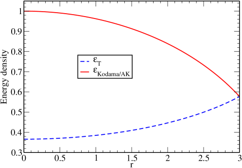
Figure 1: Energy densities for a Schwarzschild star. The energy distribution computed from either the Kodama or the almost-Killing current (continuous line), has a maximum at the center of the star that monotonically decreases until the star surfacer. In contrast, the energy density $\mathcal{E}_{T}$ (dashed line) is an increasing function that reaches the maximum value at that surface.

These energy densities are compared in Fig. 1 for a Schwarzschild star with compactness $M/R=1/3$. The energy density $\mathcal{E}_{AK}$ (continuous line), computed from either the Kodama or the almost-Killing currents, leads to a more natural energy distribution, with a maximum at the star center and monotonically decreasing as one approaches to the surface of the star. In contrast, the energy density $\mathcal{E}_{T}$ has the opposite and counter-intuitive behavior which corresponds to an increasing function that reaches the maximum value at that surface (dashed line). The geometric factor coming from the space volume element is not included in the plots.

III.2 Tolman-Bondi dust metrics

The line element of a generic (spherically symmetric) dust-filled spacetime in comoving coordinates can be written as Bondi (1947); D. Kramer and Herlt (1980)

$$ds^{2}=-dt^{2}+\frac{Y^{\prime}(r,t)^{2}}{1-k\,f(r)^{2}}~{}dr^{2}+Y^{2}(r,t)~{}d\Omega^{2}\,.$$ (38)

The area radius $Y(r,t)$ verifies, according to (22), the Friedmann-like equation

$$\dot{Y}^{2}-\frac{2\,m(r)}{Y}=-k\,f(r)^{2}\,,$$ (39)

where both the Hernández-Misner mass function $m(r)$ and $f(r)$ are arbitrary functions, although the choice of $f(r)$ is restricted by the regularity requirements of the metric. It follows from the field equations that the density $\rho$ is given by

$$4\,\pi\,\rho=\frac{m^{\prime}}{Y^{2}\,Y^{\prime}}\,.$$ (40)

The vacuum case (Schwarzschild spacetime) is then recovered where $m^{\prime}=0$.

For any dust-filled spacetime, the conservation of the stress-energy tensor amounts to the conservation of the matter current

$$J^{a}_{dust}=\rho\,u^{a}\,$$ (41)

where $u^{a}$ stands for the fluid four-velocity. The corresponding mass density is actually the matter density $\rho$. Note that the resulting mass function $M_{dust}$ is time independent (comoving coordinates) and verifies indeed

$$M^{\prime}_{dust}=\frac{m^{\prime}}{\sqrt{1-k\,f(r)^{2}}}\,,$$ (42)

which differs from the Hernández-Misner mass function unless $k=0$.

Even if there is no timelike KV in the generic case, we can define other conserved currents via either the Kodama vector or the AKV. On one hand, in comoving coordinates, the Kodama vector can be brought into the form

$$K^{a}=\sqrt{1-k\,f(r)^{2}}\,(\,1\,,-{\dot{Y}}/{Y^{\prime}}\,,0\,,0)\,.$$ (43)

The conserved Kodama current is then

$$J^{a}_{Kodama}=\sqrt{1-k\,f(r)^{2}}\,J^{a}_{dust}\,,$$ (44)

so that the Kodama energy density can be expressed as

$${\mathcal{E}}_{Kodama}=\frac{\sqrt{1-k\,f(r)^{2}}}{4\pi\,Y^{2}\,Y^{\prime}}\,m^{\prime}(r)\,,$$ (45)

which allows to recover the Hernández-Misner mass function $m(r)$ by integrating over a sphere, as we have seen before (28).

On the other hand, according to (18), the conserved AK-current is given by

$$J^{a}_{AK}=\frac{\sqrt{1-k\,f(r)^{2}}}{4\pi\,Y^{2}\,Y^{\prime}}\,(-M^{\prime},\dot{M},0,0)\,.$$ (46)

where we have introduced the potential $M(r,t)$ which coincides, up to a constant, with the mass function (20) associated to the AKV $\xi$, namely

$$M_{AK}=\frac{Y^{2}\,Y^{\prime}}{\sqrt{1-k\,f(r)^{2}}}\,\nabla^{[r}\xi^{t]}\,.$$ (47)

The energy density associated with the AKV can be then expressed as

$${\mathcal{E}}_{AK}=\frac{\sqrt{1-k\,f(r)^{2}}}{4\,\pi\,Y^{2}\,Y^{\prime}}\,M^{\prime}\,.$$ (48)

Note that, allowing for (16), the AK current can also be expressed as

$$J^{a}_{AK}=\frac{1}{4\,\pi}\,R^{a}_{b}\,\xi^{b}=\rho~{}(\,\xi^{a}+2\,u\cdot\xi~{}u^{a})\,.$$ (49)

In the non-vacuum case, the above expression can be inverted in order to obtain the components of the AKV in terms of the potential  $M$, which are given by

$$\xi^{a}=\frac{\sqrt{1-k\,f(r)^{2}}}{m^{\prime}}\,(M^{\prime},\dot{M},0,0)\,.$$ (50)

Plugging this result back into Eq. (47), we obtain a second order elliptic PDE for the potential $M(r,t)$ that ensures that $\xi$ is a true AKV in the non-vacuum case, that is

$$M-M_{s}=\frac{Y^{2}}{2\,Y^{\prime}}\,\left[~{}\partial_{t}\,\left(~{}\frac{Y^{\prime\,2}\,\dot{M}}{m^{\prime}}\right)+\sqrt{1-k\,f(r)^{2}}~{}\partial_{r}\,\left(~{}\frac{\sqrt{1-k\,f(r)^{2}}}{m^{\prime}}\,M^{\prime}\,\right)~{}\right]\,,$$ (51)

where $M_{s}$ is an integration constant. Notice that the expression (50) is undetermined in the vacuum case. For the Schwarzschild metric, however, a Killing vector exists, which actually coincides with the Kodama vector (43).

The time dependence in $M(r,t)$ is essential. The ansatz $\dot{M}=0$ is not compatible with the equation (51) in the generic case. Then, it follows from (50) that the AKV fleet of observers is tilted with respect to the comoving (geodesic) observers. The static value of both the ’number-of-particles’ mass (42) and the Hernández-Misner mass function $m(r)$ indicates that these are concepts associated to the comoving observers. From the point of view of a quasi-stationary observer, however, particles in a collapsing ball of dust are gaining kinetic energy, meaning that their mass must increase. Let us illustrate this point with a simple example

Oppenheimer-Schneider collapse

Let us consider now the case in which the matter density distribution $\rho$ is homogeneous. This can be interpreted as a cosmological solution, the pressureless case of the Friedmann-Robertson-Walker (FRW) metrics such that

$$Y=R(t)\,f(r)\,,\qquad m(r)=\frac{2}{9}\,f(r)^{3}\,.$$ (52)

If one considers the metric (38) with the parameter $k\neq-1$, the resulting spacetime corresponds to the collapse of a homogeneous ball of incoherent matter, with a vacuum exterior metric (Oppenheimer-Schneider collapse). On the other hand, the value $k=+1$ allows to choose initial data for the collapse which correspond a momentarily static configuration. We will rather consider here for simplicity the $k=0$ case, such that $R(t)=(t_{0}-t)^{2/3}$, where $t_{0}$ is the time label for the collapse to the final singularity. This allows to obtain an explicit solution of (51) which can be written as

$$M(r,t)=M_{s}+\lambda(r)~{}(t-t_{0})\,,$$ (53)

where the function $\lambda(r)$ is linear in $m(r)$, as it follows from (51).

The FRW dust interior can be matched to the vacuum exterior metric (Schwarzschild spacetime) at the radius of the star $r=r_{s}$. We can adjust the linear relation between $\lambda$ and $m(r)$ in order to match the AK mass function (53) with the Hernández-Misner mass at the surface, namely

$$M(r,t)-M_{s}=(1-t/t_{0})~{}\left[\,m(r)-M_{s}\,\right]\,.$$ (54)

This implies $\dot{M}\mid_{r_{s}}=0\,$. Therefore, according with Eq. (46), there is no flux of momentum at the surface. This means that the resulting AKV (50) is comoving at the surface.

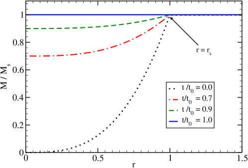
Figure 2: Time evolution of the mass function $M(r,t)$ normalized to the constant $M_{s}$ for a FRW collapsing homogeneous ball of dust in the flat case $k=0$. The surface is located $r_{s}=1.0$, where a matching with the Schwarzschild spacetime is enforced. The initial mass distribution evolves towards a constant value.

Figure (2) displays the evolution of the mass function $M(r,t)$, normalized to the constant $M_{s}$, which corresponds to the mass of the Schwarzschild spacetime (we have taken $f(r)=r$ for simplicity). We can see the expected growing behavior in time, as discussed before. The distribution in the inner region, where the FRW metric is valid, flattens out with time meaning that energy density is concentrating at the star center. At the final singularity ($t=t_{0}$), the mass function is constant everywhere.

IV Beyond Spherical Symmetry

In the following, we will explore how our AK-current approach can be used to construct conserved quantities in generic spacetimes . We begin by considering the case of rigidly rotating neutron stars, which allows to compare the resulting definition of mass obtained through either the current $\,J^{a}_{T}\,$ or the almost-Killing current $J^{a}_{AK}$. Finally, we will consider here the generic case, in which the problem to find out a suitable AKV for the current $J^{a}_{AK}$ is analyzed as a Cauchy problem.

IV.1 Rigidly Rotating Stars

The spacetime of stationary and axisymmetric (uniformly rotating) stars can be obtained by solving the hydro-Einstein equations through a multi-domain spectral code, as described in Ansorg et al. (2002, 2003). The spacetime may contain or not an ergoregion depending on the compactness of the star. The corresponding Lewis-Papapetrou coordinates are uniquely determined by the matching conditions at the surface (see  Ansorg et al. (2002); Meinel et al. (2008) for a detailed description). In the interior region we can write

$$ds^{2} = -e^{2\,U}\,(dt+a\,d\phi)^{2}+e^{-2\,U}\left[e^{2\,k}\,(d\rho^{2}+d\xi^{2})+W^{2}\,d\phi\,^{2}\right]\,.$$ (55)

where we have used a comoving coordinates system.

In this comoving frame, the stress-energy tensor is given by

$$T^{ab}=(\,\mu+p\,)\,u^{a}\,u^{b}+p\,g^{ab}\,,\qquad u^{a}=e^{-\,U}\,{\delta^{a}}_{t}\,,$$ (56)

where $\mu=\rho\,(1+\epsilon)$ is the energy density and $p$ is the pressure. It turns out that, given a particular equation of state, the conservation of the stress-energy tensor (56) yields

$$e^{U}\,\text{exp}\,\left[\int_{0}^{p}\frac{dp}{\mu+p}\right]=e^{V_{0}}=\text{const}\,.$$ (57)

The compactness of the star is therefore controlled through the parameter $V_{0}$. We have constructed several solutions with an equation of state for homogeneous matter with constant density $\mu=\text{const}$. For all the stars the value of the spin parameter is $a=J/M^{2}\approx 0.9$. The mass, rotation frequency $\Omega$ and other parameters of the solutions can be found in table I of Ref. Ruiz et al. (2012).

Here again, since the resulting spacetime is axisymmetric and stationary, we can define the conserved currents $J^{a}_{T}$ and $J^{a}_{AK}$ as before. Note however that the choice of the seed KV is not unique, as any linear combination of the two KVs is indeed a KV. The resulting conserved quantities would depend then on the selected combination. We will choose here the KV which is aligned with the fluid worldlines, so that in comoving coordinates, it can be expressed as $\,\xi^{a}=e^{U}u^{a}=\delta^{a}_{(t)}$. Therefore, according to (2) and (16), the conserved currents are

$$J_{T}^{a} = {T^{a}}_{b}\,\xi^{b}=-\mu\,e^{U}\,u^{a}\,,$$ (58)

$$J^{a}_{AK} = \frac{1}{4\pi}\,{R^{a}}_{b}\,\xi^{b}=-\,\left(\mu+3\,p\,\right)\,e^{U}\,u^{a}\,.$$ (59)

The associated energy densities are therefore

$$\mathcal{E}_{T} = -n_{a}J_{T}^{a}=\mu\,A\,e^{U}\,,$$ (60)

$$\mathcal{E}_{AK} = -n_{a}J^{a}_{AK}=\left(\mu+3\,p\,\right)A\,e^{U}\,,$$ (61)

where $A=n\cdot u~{}$ is the Lorentz factor.

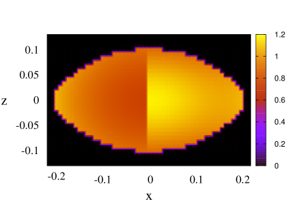
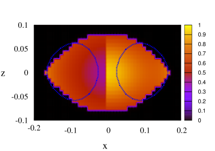
Figure 3: Comparison between the energy densities $\mathcal{E}_{T}$ and $\mathcal{E}_{AK}$ for a rapidly rotating neutron stars with and without ergosphere (right and left panel, respectively) on the vertical plane. The dotted line corresponds to the ergosphere surface, which has a torus-like shape. In both configuration, the energy density $\mathcal{E}_{T}$ is displayed on the negative $x$ axis, while that AK energy density is plotted on the positive side. The $\mathcal{E}_{AK}$ distribution has a maximum at the center of the star that monotonically decreases until the surface of the star while the $\mathcal{E}_{T}$ distribution corresponds to a increasing function that reaches its maximum value at the surface of the star.

In figure 3 we compare the resulting mass-energy densities on a vertical plane for the two cases $V_{0}=-0.8$ and $V_{0}=-1.25$ (see table I of Ref. Ruiz et al. (2012)). The configuration displayed in the left panel corresponds to a standard neutron star with constant density while the configuration displayed in the right panel corresponds a neutron star with a torus-shaped ergoregion (signaled by a dotted line). The $\,\mathcal{E}_{T}\,$ energy density is displayed on the negative $x$ axis, while that $\mathcal{E}_{AK}$ energy density is plotted on the positive side. Notice that in both star models (with and without ergosphere) the $\,\mathcal{E}_{T}\,$ energy density has lower values close to the axis that increases towards the surface of the star whereas the AK energy density has a maximum at the center that decreases monotonically outward until the surface. This is the same behavior as the one obtained in section III for the spherical case. The conclusion is again that the energy density $\mathcal{E}_{AK}$ matches the physically expected profile whereas $\,\mathcal{E}_{T}\,$ has a counter-intuitive behavior.

IV.2 Generic Spacetimes

As we have seen in section II, the AKE (12) can always be solved in a generic spacetime provided that $\mu\neq 2$. Nevertheless, in this paper we are considering precisely the special case $\mu=2$ because just in this case we obtain a suitable energy current $J_{AK}$.

Let us look now at the definition of the current $J_{AK}$ which is given in Eq. (18). It can be interpreted as the AKV differential equation for the $\mu=2$ case namely

$$\nabla_{b}\nabla^{[a}\xi^{b]}={R^{a}}_{b}\,\xi^{b}\,.$$ (62)

It is easy to show that the time derivative of the time component of the vector field $\xi$ does not appear in the above system. Only the antisymmetric combination of first derivatives is involved. Therefore, the principal symbol becomes singular in Fourier space Bona et al. (2005). Although we have four second order equations for the four $\xi^{a}$ components, only the space components $\xi^{i}$ of the AKV can be computed from their evolution equations in a straightforward way.

This opens the door to consider the time component of (14) as a constraint, in the same spirit as in the free evolution approach in numerical relativity. Let us consider the quantities ${\cal C}^{a}$ representing deviations from the Eq. 62:

$$\nabla_{b}\nabla^{[a}\xi^{b]}={R^{a}}_{b}\,\xi^{b}+{\cal C}^{a}\,.$$ (63)

If we take now the divergence of this vector relation, we obtain

$$\nabla_{a}{\cal C}^{a}=-\nabla_{a}({R^{a}}_{b}\,\xi^{b})=-4\pi\,\nabla_{a}J_{AK}^{a}\,.$$ (64)

Therefore, the conservation of the AK-current amounts to the conservation of the deviations ${\cal C}^{a}$, that is

$$\partial_{0}(\sqrt{g}\,{\cal C}^{0})+\partial_{i}(\sqrt{g}\,{\cal C}^{i})=0\,.$$ (65)

In the vacuum case, where $J_{AK}$ vanishes, it would be enough to impose the constraint ${\cal C}^{0}=0$ in the initial data in order to ensure that it will hold during the whole evolution, provided that we enforce ${\cal C}^{i}=0$ by computing the space components $\xi^{i}$ in the right way, namely:

$$\nabla_{b}\nabla^{[b}\xi^{i]}+{R^{i}}_{b}\,\xi^{b}=0\,.$$ (66)

At the same time, one would get the some gauge freedom for choosing $\xi^{0}$. Notice that in vacuum, the expression (62) is equivalent to the first set of Maxwell equations, in which the vector field $\xi$ would play the role of the electromagnetic potential. Nevertheless, in the non-vacuum case the problem becomes circular since the conservation of $J_{AK}$ is not granted unless $\xi$ is a true AKV and this requires indeed ${\cal C}^{0}=0$. There is no simple alternative to using the elliptic-type equation

$$\nabla_{a}\nabla^{[a}\xi^{0]}+{R^{0}}_{a}\,\xi^{a}=0\,,$$ (67)

for computing the $\xi^{0}$ component. This (partially) elliptic nature of the problem showed up yet in the spherical dust case (see section III), where we used the mass function as a sort of potential for $\xi$, leading to the elliptic equation (51). In the generic (non-spherical) case, the system of AKV equations is of a mixed elliptic-hyperbolic nature, like the ones considered in recent Numerical Relativity developments Cordero-Carrion and Cerda-Duran (2012). Studying the mathematical properties of this system is beyond the scope of this work.

V Conclusions

We have proposed a new conserved current, describing energy densities of non-gravitational origin, namely

$$J^{a}_{AK}=\frac{1}{4\pi}\,{R^{a}}_{b}\,\xi^{b}\,.$$

We called it almost-Killing current because it requires (a particular case of) a timelike almost-killing vector $\xi$ in order to ensure conservation. The physical meaning of such current is of course related with the physical meaning of the AKV itself.

As a first instance, we have explored the stationary/static case, in which the AKV can be chosen to be a Killing vector, which allows us to obtain the well known current

$$J^{a}_{T}={T^{a}}_{b}\,\xi^{b}\,.$$

Our results show that the energy density profiles obtained with $J_{AK}$ are the expected ones: the profile reaches a maximum value at the center of the star and decreasing outwards until the surface of it. In strong contrast, the energy associated with $J_{T}$ corresponds to an increasing function which reaches its maximum value at the surface of the star. We have shown these opposed behaviors for the Schwarzschild (constant-density) star, as well as for rigidly rotating stationary stars which can contain an ergoregion Ansorg et al. (2002). The unphysical behavior of $J_{T}$ is not a surprise. It is well known that, in order to recover the Hernández-Misner mass function Hernandez Jr and Misner (1966), the Killing vector must be rescaled in a non-trivial way (Kodama vector). Our results confirm that the proposed current $J_{AK}$ provides a possible solution for that problem in both the static and the stationary cases.

Of course, there is an inherent ambiguity in our approach, as any AKV can be used as a seed for generating the corresponding conserved current. The stationary case provides a good reference in this sense, because the ambiguity in the choice of the seed AKV is solved by selecting precisely the timelike KV. In the stationary axisymmetric case, however, some ambiguity reappears since the choice of the KV is not unique. This ambiguity problem grows in the generic non-stationary case, which is a bigger challenge in many respects. Note however that in the spherical case, where a mass function $M_{AK}$ can be explicitly computed, one gets a simple generalization of the Kepler law (31), strongly supporting the physical interpretation of our results, and this is so for any selection of the seed AKV.

We have considered the whole class of Tolman-Bondi solutions for spherical balls of dust D. Kramer and Herlt (1980). In comoving coordinates, the Hernández-Misner mass function for this case is time-independent, $m=m(r)$, suggesting a baryonic mass interpretation, although it is different from the standard result for dust, obtained from the matter current

$$J^{a}_{dust}=\rho\,u^{a}\,.$$

The mass function $M(r,t)$ associated to the proposed current $J_{AK}$ depends instead on time in the generic case, which is the expected behavior for the energy density in a dynamical collapse scenario, where the kinetic energy of particles is varying in time. The static character of the Hernández-Misner mass suggests that it is linked to the comoving observers, which are not quasi-stationary in the generic case. We have shown that the proposed mass function can be used as a potential, so that the AKV equations can be expressed as a single elliptic-type equation for $M(r,t)$.

In the generic, non-spherical, case the AKV set of equations is of a mixed elliptic-hyperbolic type, like the ones considered in recent Numerical Relativity developments Cordero-Carrion and Cerda-Duran (2012). We are currently working on the properties of this system with a view to devising suitable coordinate systems, adapted to the type of conservation laws considered in the paper.