Disturbance accelerates the transition from low- to high- diversity state in a model ecosystem

Abstract

The effect of disturbance on a model ecosystem of sessile and mutually competitive species [Mathiesen et al. Phys. Rev. Lett. 107, 188101 (2011); Mitarai et al. Phys. Rev. E 86, 011929 (2012) ] is studied. The disturbance stochastically removes individuals from the system, and the created empty sites are re-colonized by neighbouring species. We show that the stable high-diversity state, maintained by occasional cyclic species interactions that create isolated patches of meta-populations, is robust against small disturbance. We further demonstrate that finite disturbance can accelerate the transition from the low- to high-diversity state by helping creation of small patches through diffusion of boundaries between species with stand-off relation.

I Introduction

The high-diversity of sessile species in a limited space, observed in for example crustose lichen Harris (1996); Jettestuen et al. (2010), coral reef Buss and Jackson (1979); Volkov et al. (2007) and epifaunal species Kay and Keough (1981) ecosystems, is one of the unsolved puzzle in ecology. Interestingly, these examples often lacks an obvious dominant species in their competition Harris (1996); Jettestuen et al. (2010); Buss and Jackson (1979); Kay and Keough (1981). Instead, many competitive equivalent species, stand-offs (i.e. a boundary between two species stays still), and cyclic (non-transitive) relationships are observed, which should contribute the maintenance of the high biodiversity.

Cyclic relations of species are extensively studied Gilpin (1975), which gives coexistence of oscillating populations for some time, but in a well mixed system noise due to finite population eventually leads to the extinctions of the species and dominance of one or a few species Reichenbach et al. (2006), unless the strength of the interaction between the species and the selection pressure is chosen in the range that allows coexistence Claussen and Traulsen (2008). Recent work Knebel et al. (2013) provides the coexistence criteria of a given interaction network in well-mixed system with conservative dynamics. By combining cycles with space to limit the interaction to local neighbors, the coexistence is found to be stabilized Boerlijst and Hogeweg (1991); Laird and Schamp (2006); Szabó and Czárán (2001); Czárán et al. (2002); Kerr et al. (2006); Perc and Szolnoki (2007); Lütz et al. (2012); Roman et al. (2013). For sessile species, the non-transitive relationships between species are found to prolong the the coexistence time than hierarchical relationships Buss and Jackson (1979); Jackson and Buss (1975); Karlson and Buss (1984).

Mathiesen et al. Mathiesen et al. (2011) proposed a spatial model ecosystem of sessile and mutually excluding organisms, inspired by crustose lichen communities. The model considers the overgrowth or allelopatic interaction between species, that allows a species to invade a space occupied already by another species. Slow introduction of new species to the system is allowed, while stochastic extinction can also happen due to the finite population, therefore the number of the species in the system is not fixed a priori in the model cul . In the limit of slow introduction rate, it was demonstrated that the model showed a discontinuous transition from the low- to high-diversity state as the invasion interaction is reduced, hence the fraction of stand-offs increased. In the high-diversity state, the spatial distribution of species is self-organized into fragmented patches, and species implicitly protect each other from the direct contact with the “competitively superior” species to allow stable coexistence. It has been demonstrated that cyclic relationships of length 4 to 6 are necessary for maintenance of diversity through creation of patches Mitarai et al. (2012).

One of the biologically important extensions of the model is to include random disturbance from environment and/or natural deaths of the individuals. The disturbance creates empty space, which can be recolonized from neighboring species Karlson and Buss (1984). Such a disturbance creates free space available for all species, and at the same time the species with the biggest population may be hit more often by disturbance. Therefore, disturbance may help inferior species to compete with dominant species Dayton (1971); Paine (1974). When the disturbance is very high, the species interaction becomes irrelevant for the ecosystem Karlson and Buss (1984), and a large influx of new species becomes necessary to keep the diversity. The biodiversity in a community obtained by balance between the influx of new species and random extinction due to stochastic growth and death without species interaction is discussed in the neutral theory of biodiversity Hubbell (2001); Volkov et al. (2003, 2007).

Though the high-diversity state of the model in ref. Mathiesen et al. (2011) is realized as the balance between the slow influx of new species and the occasional extinction, it is different from the neutral theory situation because the high-diversity state maintained in the small influx limit relies on the spacial structure created by the species interactions. The effect of disturbance was tested before Mathiesen et al. (2011) by emptying a fraction of sites prior to the introduction of new species, and it was found that high diversity is maintained as long as the removal is less that 10%. However, the systematic study on either the stochastic disturbance on the dynamics or the relation between the disturbance and influx of new species has not been performed yet. Since the species interaction becomes irrelevant in the large disturbance limit, our interest is in the effect of small but finite disturbance to the model behavior.

In this paper, we study the ecosystem model Mathiesen et al. (2011); Mitarai et al. (2012) with a finite disturbance rate. We show that, when the disturbance rate is small enough for a given introduction rate of new species, the clear distinction between the low and high-diversity states and the sharp transition between them are maintained. We further demonstrate that the disturbance can even enhance the transition from the low- to high-diversity state, by mediating the fragmentation of the species into spatially separated patches.

II Model

II.1 Model algorithm

The ecosystem is modelled on a two-dimensional square lattice of the linear size $L$ with variable number of species, where each site can either be empty or hold at most one species. The species interactions are characterized by a randomly assigned directed network, and the network connectivity is parametrized by the probability $\gamma$ (see below). The interaction takes place only among spatially neighboring species. New species are introduced with a constant rate $\alpha_{N}$ per site ($\alpha_{N}\times L^{2}$ per system), while randomly chosen sites are emptied by disturbance with a rate $\omega_{N}$ per site ($\omega_{N}\times L^{2}$ per system).

Each update of our model consists of the following three possible events:

1. Introduction of new species. With probability $\alpha_{N}$, choose a random lattice site $j$. (a) If the site $j$ is empty, then a new species $s$ is introduced at the site $j$, and assigned random interactions $\Gamma(s,u)$ and $\Gamma(u,s)$ with all existing species $u$ in the system. Each of these interactions are assigned value 1 with probability $\gamma$, and otherwise set to $0$. $\Gamma(s,u)=1$ indicates that the species $s$ can invade the species $u$, while $s$ cannot invade $u$ if $\Gamma(s,u)=0$ (See invasion rule below). (b) If instead the site $j$ is occupied already by another species $v$, then a new species $s$ is introduced with probability $\gamma$, which is the probability that the species $s$ can invade the species $v$. When $s$ is introduced, $\Gamma(s,u)$ and $\Gamma(u,s)$ for all existing species $u$ in the system are assigned in the same way as (a), and then $\Gamma(s,v)$ is set to $1$.

2. Disturbance. With probability $\omega_{N}$, choose a lattice site $i$ randomly. If there exist a species on the site $i$, make the site $i$ empty, hence the population of the species will be reduced by one.

3. Invasion. Choose a random lattice site $i$. If there is a species $s(i)$ at the site $i$, choose one of its 4 neighbor sites $j$ randomly. If the site $j$ is empty, or if there is a species $s(j)$ at the site $j$ and $s(i)$ can invade $s(j)$ (i.e. $\Gamma[s(i),s(j)]=1$), then the site $j$ will be updated to be occupied by the species $s(i)$ by setting $s(j)=s(i)$.

One time unit is defined as $L^{2}$ repeats of the procedures 1 to 3. Therefore, per time unit, on average each site makes one attempt to invade a neighbor, $\alpha_{N}\times L^{2}$ new species attempt to enter the system, and $\omega_{N}\times L^{2}$ individuals are removed. Since $\alpha_{N}$ and $\omega_{N}$ are defined as a probability for the introduction and the death occur per time unit, respectively, they can take any value between 0 and 1. $\omega_{N}=0$ recovers the original ecosystem model in Mathiesen et al. (2011); Mitarai et al. (2012).

Because of the random assignment of the interaction matrix $\Gamma$, there will be no dominant species. For a given pair of species $(s,u)$, one of them can be dominant ($\Gamma(s,u)=1$ and $\Gamma(u,s)=0$ or vice versa), or they can be competitively equivalent. Note that there are two kinds of competitive equivalence: it can be with active invasion to each other ($\Gamma(s,u)=\Gamma(u,s)=1$), or with the stand-off relation ($\Gamma(s,u)=\Gamma(u,s)=0$). The stand-off relation increases for smaller $\gamma$, mediating the stable coexistence of many species when $\omega_{N}=0$.

II.2 Simulation setup

In the following simulations, we use $L=200$ under periodic boundary condition. System size dependence was was studied before at $\omega_{N}=0$ Mathiesen et al. (2011) and will be summarized in subsection III.1. $L=200$ was found to be enough to observe the transition to the high-diversity state. Initial condition is an empty system, unless otherwise noted.

In order to reduce the computation time, some of the simulations with small values of $\alpha_{N}$ and $\omega_{N}$ were performed by the event-driven type algorithm, where the possible events are listed and time to the next event was drawn accordingly from the exponential distribution. This gives statistically the same results as the described random sequential updates.

III Results

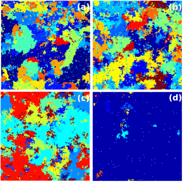
Figure 1: (color online) Snapshots of in the high-diversity state with $\alpha_{N}=2.5\times 10^{-7}$, $\gamma=0.03$, with various death rate $\omega_{N}$. (a) $\omega_{N}=0$, (b) $\omega_{N}=2.5\times 10^{-5}$, (c) $\omega_{N}=2.5\times 10^{-4}$, (d) $\omega_{N}=2.5\times 10^{-3}$. The empty sites are shown as white, and the sites with species are filled.

III.1 Summary of the behavior without the disturbance

We first summarize the relevant findings in the previous papers for no disturbance ($\omega_{N}=0$) Mathiesen et al. (2011); Mitarai et al. (2012), to clearly demonstrate the effect of the disturbance later.

In the no-disturbance case, the time-averaged diversity (number of species in the system) $\langle D\rangle$ was found to decrease to one as $\alpha_{N}\to 0$ for $\gamma>\gamma_{c}\approx 0.06$, while for $\gamma<\gamma_{c}$, $\langle D\rangle$ converges to a finite non-zero value as $\alpha_{N}\to 0$. In the limit of $\alpha_{N}\to 0$, or the quasistatic version of the model where a new species is inserted into the system only after all the activity in the system has stopped qua , the state with the diversity $D=1$ is an absorbing state, since newly added species will simply replace the previous species. When the simulation is started from the high diversity state in the quasi-static limit, the system stably remains in the high-diversity state for $\gamma<\gamma_{c}$, while for $\gamma>\gamma_{c}$ the diversity goes down to one. Namely, the diversity shows a discontinuous transition as a function of $\gamma$ in the $\alpha_{N}\to 0$ limit.

When $\alpha_{N}$ is finite but small enough ($\alpha_{N}\leq 2.5\times 10^{-7}$), the high-diversity state is mono-stable for $\gamma<\gamma_{c}$, while the diversity $D$ shows clear bi-stability between the high-diversity state and the low-diversity state for $\gamma>\gamma_{c}$, and hence the transition in the long-time average $\langle D\rangle$ appears softer as a function of $\gamma$ for non-zero $\alpha_{N}$. When $\alpha_{N}$ is large, the difference between the high- and the low-diversity state is smeared out even without taking long-time average, since the high introduction of species forces the system to contain many species all the time.

A snapshot of the system in the high-diversity state with $\omega_{N}=0$, $\alpha_{N}=2.5\times 10^{-7}$, $\gamma=0.03$ for $L=200$ is shown in Fig. 1a. We can see that the species are separated into many patches created by species interactions. When $\gamma<\gamma_{c}$, the system stabilizes to the situation where most of the species cannot invade their neighbors, and slow introduction of new species gives local updates of the species distribution. The spatial separation due to the patch formation implicitly protect each other from the “competitively superior” species to allow the high diversity in the system.

The maximum patch-size has a well-defined cut-off around $10^{4}$ sites in area for small enough $\alpha_{N}$ for $\gamma<\gamma_{c}$, for $L\geq 200$. If the total system size $L$ is smaller than $\approx 150$, the high-diversity state is not stable because the large patches interfere with the system size, and we do not observe the transition. For a large enough system size, the transition point $\gamma_{c}$ does not depend on $L$, and the diversity increases linearly with the total system’s area, $L^{2}$.

We have also shown Mitarai et al. (2012) that cyclic relationships, especially of the length 4 to 6, are needed to maintain the high diversity. Here, for example cyclic relation of length 4 means the relation $A\to B\to C\to D\to A$, where $X\to Y$ represents that the species $X$ can invade the species $Y$. Such cyclic relationships give complex spatiotemporal dynamics, and when some of the species go extinct due to the stochasticity, many patches can be left behind. In the case of cycle of length 4, for example, if A dies out first, it is likely that B displaces C before C can displace D since $B$ will not be attacked any more; in the end patches of B and D will be left and they will coexist with stable boundary between them. Obviously the cycles of length 2 and 3 do not leave patches, while longer cycles are less likely to be activated. It has been shown that, when $\omega_{N}=0$, the high-diversity state is not stable without cycles of length $4-6$ in the $\alpha_{N}\to 0$ limit for $\gamma=0.025$ Mitarai et al. (2012), suggesting the necessity of the patch creation through the cyclic relations.

III.2 Effect of the the disturbance

III.2.1 Average diversity

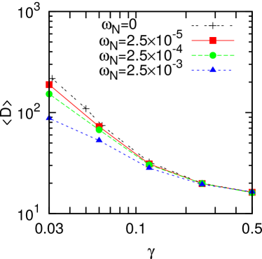
Figure 2: (color online) Long-time average of the diversity $\langle D\rangle$ as a function of $\gamma$. $\alpha_{N}=2.5\times 10^{-6}$, and results for $\omega_{N}=0,2.5\times 10^{-5},2.5\times 10^{-4},$ and $2.5\times 10^{-3}$ are shown. The average was taken from the data of the duration $9\times 10^{6}$ time steps or longer. The standard error is smaller than the symbol size.

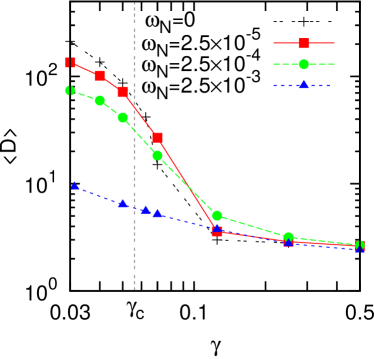
Figure 3: (color online) Long-time average of the diversity $\langle D\rangle$ as a function of $\gamma$. $\alpha_{N}=2.5\times 10^{-7}$, and results for $\omega_{N}=0,2.5\times 10^{-5},2.5\times 10^{-4},$ and $2.5\times 10^{-3}$ are shown. The average was taken from the data longer than the following duration; For $\omega_{N}=0$, $\gamma\leq 0.125$: $7\times 10^{8}$ time steps. For $\omega_{N}=0$, $\gamma=0.25$: $1\times 10^{8}$ time steps. For $\omega_{N}=0$, $\gamma=0.5$: $1.9\times 10^{7}$ time steps. For $\omega_{N}=2.5\times 10^{-5}$, $\gamma\leq 0.25$: $1\times 10^{8}$ time steps. For $\omega_{N}=2.5\times 10^{-5}$, $\gamma=0.5$: $8\times 10^{7}$ time steps. For $\omega_{N}=2.5\times 10^{-4}$, $\gamma\leq 0.125$: $1\times 10^{8}$ time steps. For $\omega_{N}=2.5\times 10^{-4}$, $\gamma=0.25$: $9\times 10^{7}$ time steps. For $\omega_{N}=2.5\times 10^{-4}$, $\gamma=0.25$: $5\times 10^{7}$ time steps. For $\omega_{N}=2.5\times 10^{-3}$, $\gamma\leq 0.075$: $9\times 10^{7}$ time steps. For $\omega_{N}=2.5\times 10^{-3}$, $\gamma=0.25,0.5$: $9\times 10^{6}$ time steps. The standard error is smaller than the symbol size.

Now we move on to the case with the non-zero disturbance rate, $\omega_{N}$. Figures 1b-d show snapshots for $\alpha_{N}=2.5\times 10^{-7}$ and $\gamma=0.03$ with $\omega_{N}=2.5\times 10^{-5},2.5\times 10^{-4}$, and $2.5\times 10^{-3}$, respectively, in the high-diversity state. When the disturbance happens at the boundary between two stand-off species, the empty sites will be filled by one of the neighboring species, resulting in slow diffusion of the boundary. This situation is the same as the voter model Dornic et al. (2001), where a smooth interface roughens due to the lack of the surface tension. This makes the boundary between species more rugged and leads to elimination of the patches as $\omega_{N}$ increases.

We then studied the $\alpha_{N}$, $\gamma$, and $\omega_{N}$ dependence of the time averaged diversity $\langle D\rangle$. With finite $\omega_{N}$ and large enough $\alpha_{N}\geq 1.25\times 10^{-6}$, $\langle D\rangle$ decrease with increasing $\omega$ from zero for any fixed value of $\gamma$. An example is given in Fig. 2 for $\alpha_{N}=2.5\times 10^{-6}$ with various values of $\omega_{N}$. This $\alpha_{N}$ is large enough to dominate the system’s diversity for $\omega_{N}=0$ case to smear out the difference between the high-diversity state and the low-diversity state. The monotonic dependence on $\omega_{N}$ suggest that $\omega_{N}$ is simply counteracting the diversity by accelerating the extinction through random death of individuals.

When $\alpha_{N}=2.5\times 10^{-7}$ and $\gamma<\gamma_{c}$, $\langle D\rangle$ again decreases monotonically with increasing $\omega_{N}$ as shown Fig. 3. This is expected because the disturbance results in the fluctuation of the stable boundary between species with stand-off relation, as depicted in Fig. 1, namely too large $\omega_{N}$ destabilize the high-diversity state. When $\gamma=0.03$, for example, the system is monostable in the high-diversity state for $\omega_{N}<2.5\times 10^{-4}$ over $10^{8}$ time steps, but it shows bistability between the high- and low-diversity states when $\omega_{N}$ exceeds $\omega_{N}<5\times 10^{-4}$. Destabilization of the high-diversity state for $\gamma<\gamma_{c}$ also occurs when $\omega_{N}$ is kept finite and $\alpha_{N}$ is decreased. For $\gamma=0.03$ and $\omega_{N}=2.5\times 10^{-5}$, the high-diversity state was stable for $\alpha_{N}=2.5\times 10^{-7}$ over $10^{8}$ time steps, but became clearly unstable when $\alpha_{N}=2.5\times 10^{-9}$.

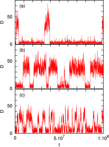
Figure 4: (color online) Time dependence of diversity $D$ in the bistable region, $\alpha_{N}=2.5\times 10^{-7}$ and $\gamma=0.07$. (a)$\omega_{N}=0$, (b)$\omega_{N}=2.5\times 10^{-5}$,(c)$\omega_{N}=2.5\times 10^{-4}$. The frequency to reach the high-diversity state increases with $\omega_{N}$, while the value of the diversity in the high-diversity state weakly decreases with $\omega_{N}$.

Interestingly, we found that $\langle D\rangle$ shows a non-monotonic dependence on $\omega_{N}$ for $\alpha_{N}=2.5\times 10^{-7}$ and $\gamma>\gamma_{c}$ (Fig. 3). Especially, when $\gamma$ is just above $\gamma_{c}$, where the $\omega_{N}=0$ systems show bistability between the high- and low-diversity states, $\langle D\rangle$ increases when $\omega_{N}$ is increased from zero to $2.5\times 10^{-5}$ and then decreases with increasing $\omega_{N}$ further.

III.2.2 Transition rates between the low-diversity state and the high-diversity state

The non-monotonic dependence of the time-averaged diversity $\langle D\rangle$ on $\omega_{N}$ is due to the difference in the transition rates between the low- and high-diversity states. As shown in Fig. 4 for $\alpha_{N}=2.5\times 10^{-7}$ and $\gamma=0.07$, increasing $\omega_{N}$ slightly decrease the value of $D$ in the high-diversity state, but the effect is very weak. However, the transition rates for both from the low- to high-diversity state and the high- low-diversity state are significantly increased with increasing $\omega_{N}$. Especially, the enhancement of the transitions from the low- to high-diversity state is significant from $\omega_{N}=0$ case to the $\omega_{N}=2.5\times 10^{-5}$ case, which gives larger probability to be in the high-diversity state resulting in the higher value for $\langle D\rangle$.

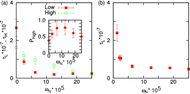
Figure 5: (color online) (a) Average transition time from the low- to high-diversity state $\tau_{L}$ and from the high- to low-diversity state $\tau_{H}$ as a function of $\omega_{N}$ in the bistable region, $\alpha_{N}=2.5\times 10^{-7}$, $\gamma=0.07$. The transition between the high- and low-diversity states by using two threshold for the diversity: $D_{l}=1$ as threshold for low diversity and $D_{h}(\omega_{N})$ as the threshold for high diversity. In order to determine $D_{h}(\omega_{N})$, we first define the high-diversity state as the state where $D$ has distinctly high diversity $D>1$ for longer than $10^{5}$ time steps, and then calculated $D_{h}(\omega_{N})$ as the average over the diversity over this period. We then define a switching event from the low- to high-diversity state when $D$ exceeds $D_{h}$, while the reverse switching happens when $D$ reaches $D_{l}$. The life time of the low- (high-) diversity state $\tau_{L}$ ($\tau_{H}$) is defined as the time between the high to low (low to high) switching event and the low to high (high to low) switching event com . Inset: Probability to be in the high-diversity state $P_{high}\equiv\tau_{H}/(\tau_{H}+\tau_{L})$, which has maximum at $\omega_{N}\approx 10^{-4}$. (b) Average transition time from the low- to high-diversity state $\tau_{L}$ as a function of $\omega_{N}$ with $\alpha_{N}=2.5\times 10^{-7}$ and $\gamma=0.03$, where the high-diversity state is monostable within the simulated timescale. In this case, we start from $D=0$ and measure the time it takes before $D$ reaches the high diversity state value $D_{h}$.

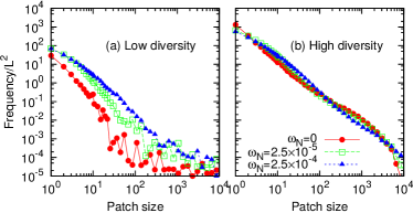
Figure 6: (color online) Patch size distribution for $\alpha_{N}=2.5\times 10^{-7}$ and $\gamma=0.07$ with $\omega_{N}=0,2.5\times 10^{-5},$ and $2.5\times 10^{-4}$. (a) For low-diversity state. (b) For high-diversity state.

We quantify the average life time of the low- (high-) diversity state $\tau_{L}$ ($\tau_{H}$) in the bistable regime as a function of $\omega_{N}$ (Fig. 5a). We see that $\tau_{L}$ quickly decreases about 9 fold when $\omega_{N}$ increases from zero to $5\times 10^{-5}$, and then saturate. $\tau_{H}$ also decrease with $\omega_{N}$, but the change is slower. This results in a peak of the probability to be in the high-diversity state $P_{high}=\tau_{H}/(\tau_{H}+\tau_{L})$, leading to the non-monotonic dependence of $\langle D\rangle$ to $\omega_{N}$.

The faster transition from the low- to high-diversity state is also seen in the monostable high-diversity regime. Figure 5b shows $\tau_{L}$ with $\alpha_{N}=2.5\times 10^{-7}$, $\gamma=0.03$, for $0<\omega_{N}\leq 2.5\times 10^{-4}$. Within this parameter range, the high-diversity state is monostable over at least $10^{8}$ time steps. We measured the life time to the low-diversity state $\tau_{L}$ by starting from an empty system and averaged over at least 20 events. The resulting life time of the low-diversity state $\tau_{L}$ shows again a sharp drop as $\omega_{N}$ increases from 0 to $\sim 5\times 10^{-5}$ and then converges to a constant number as $\omega_{N}$ further increases.

We hypothesize that this acceleration of the transition to the high diversity by $\omega_{N}$ is because disturbance-induced fluctuation of the boundaries creates more patches or meta-populations. Suppose that the diversity is low, but still by chance a few species are coexisting, each of them occupying one patch (a connected region) in the system and they cannot invade each other. The boundaries between species will diffuse due to the disturbance, creating more and more small isolated patches. These additional patches allow the system to host more species as species in a patch is replaced with a new species, helping the system to reach high-diversity state.

Figure 6a shows the patch-size distribution for $\alpha_{N}=2.5\times 10^{-7}$ and $\gamma=0.03$, obtained from the snapshots before the system reaches the high-diversity state. We clearly see that the systems with non-zero $\omega_{N}$ have more patches than the system with $\omega_{N}=0$, especially many of small patches with size $1$ to $10$. In the high-diversity state for the system with the same parameters (Fig. 6b), on the other hand, we see that more and more patches of size 1 are removed as $\omega_{N}$ increases, which contribute to the destabilization of the high-diversity state by $\omega_{N}$.

III.3 Necessity of the cyclic relationship for the high-diversity state

As summarized in subsection III.1, it has been shown Mitarai et al. (2012) that, for $\omega_{N}=0$, cyclic relationships, especially of the length 4 to 6, are needed to maintain the high diversity. We here investigate whether the patch creation by disturbance is enough or the system needs further creation of the patches through species interactions to keep the system in the high-diversity state.

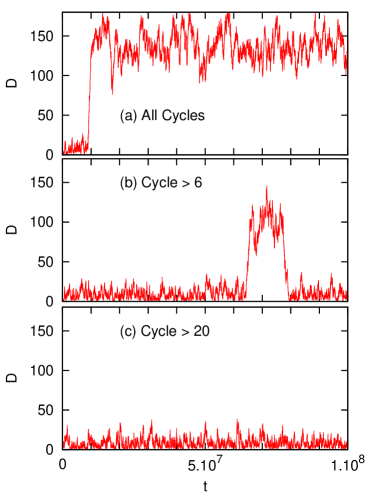
Figure 7: (color online) Effect of cycles for $\alpha_{N}=2.5\times 10^{-7}$ and $\gamma=0.03$ with $\omega_{N}=2.5\times 10^{-5}$ on the time dependence of $D$. (a) All cycles lengths are allowed ($C_{mim}=0$). (b) Cycles of length longer than 7 are allowed ($C_{mim}=6$). (c) Cycles of length longer than 20 are allowed ($C_{mim}=20$).

In order to test this, we performed simulations with cycles of various degree by the following way Mitarai et al. (2012): When a new species was introduced, the corresponding entries in the interaction matrix $\Gamma$ were determined according to the given value of $\gamma$ , but if it would result in a cyclic relationship of length less than $C_{min}$, the species was rejected, and another new species was introduced, which again was assigned random interactions according to $\gamma$.

Figures 7(a), (b), and (c) show the time series of the diversity $D$ for $C_{min}=0$ (i.e., the original model with all the cycles), $C_{min}=6$, and $C_{min}=20$, respectively, with $\alpha_{N}=2.5\times 10^{-7}$, $\gamma=0.03$, and $\omega_{N}=2.5\times 10^{-5}$. When all the cycles are allowed, the transition to the high $D$ state occurs rather fast and it is monostable (Fig.7a). The system can still go to the high-diversity state when only the cycles of length longer than 7 are allowed, but the state is not stable (Fig.7b). When only the cycles of length longer than 20 are allowed, the transition to high-diversity state did not happen within $2\times 10^{8}$ time steps (Fig.7c shows only half of the time series).

IV Summary

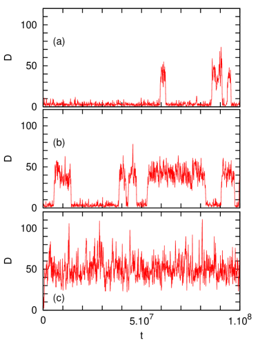
Figure 8: (color online) Time dependence of diversity $D$ in the bistable region, $\alpha_{N}=2.5\times 10^{-7}$ and $\gamma=0.07$, with various mobility rate $\mu_{N}$. The mobility is defined by replacing the disturbance step 2. in the algorithm in section II.1 with the following step: 2’. Mobility. With the probability $\mu_{N}$, select a neighboring pair of sites randomly, and exchange the species between the chosen sites. (a)$\mu_{N}=2.5\times 10^{-8}$, (b)$\mu_{N}=2.5\times 10^{-7}$, (c)$\mu_{N}=2.5\times 10^{-6}$. The frequency to reach the high-diversity state increases with $\mu_{N}$, while the transition to the low diversity state is suppressed with increasing $\mu_{N}$.

We studied a model ecosystem with a finite rate of disturbance. The transition to the high-diversity state in the ecosystem model Mathiesen et al. (2011); Mitarai et al. (2012) is shown to be robust against the finite disturbance rate $\omega_{N}$; as long as $\omega_{N}$ is small enough compared to the introduction rate of the new species $\alpha_{N}$, the clear separation between the high-diversity state and the low-diversity state is observed, and the high-diversity state is stable over long time for small enough $\gamma$.

We demonstrated that, even though the disturbance lowers the diversity at the high-diversity state, it can accelerate the transition from the low- to high-diversity state. We also found that the cyclic interactions of proper lengths are still necessary for both the stable high-diversity state and the acceleration of transition to the high diversity by $\omega_{N}$. These results may understood as follows: The disturbance results in the diffusion of the boundary between species with stand-off relation, which creates small patches that can host more species. The patches created by the disturbance at the low-diversity state accelerate the transition to the high-diversity state by increasing the chance of cycles activated in the system. In this way small disturbance can promote the high-diversity state.

The effect of the disturbance studied here may be expected to be close to the effect of local mobility Reichenbach et al. (2007) of two neighboring individuals able to swap their position with a small probably, because both makes a boundary between species diffuse. Preliminary result of the model with small $\alpha_{N}$ with local mobility showed the enhancement of the transition to the high-diversity state for the small mobility (Fig. 8). However, there is a qualitative differences between the mobility and the disturbance: the mobility does not directly decrease the population of each species. Therefore, the small mobility does not enhance the transition from the high-diversity state to the low-diversity state. It is also known that the mobility will enhance the formation of ”defensive alliances”, by promoting the segregation of the species so that the ones without direct competition appears more often next to each other Szabó and Czárán (2001); Roman et al. (2013). This is also expected to promote the high diversity by reducing the extinction due to species interactions. At the same time, we have demonstrated in the previous paper Mathiesen et al. (2011) that the random neighbor version of the model, where the invasion step happens between two randomly chosen sites irrespective of the distance between them, does not support the high diversity state. The random neighbor situation should correspond to the high mobility limit, therefore non-monotonic dependence of the diversity on the mobility may be observed. This should be clarified in the future work.

The mobility in the longer distance, on the other hand, is also natural to take into account, when considering lichen spreading spores via wind Muñoz et al. (2004) or coral spreading with the water circulation Wolanski et al. (1989). In the present model, the parameter $\alpha_{N}$ is interpreted as immigration of a new species from an external environment. It will be interesting to compare the present model and the model with global mobility in a large system size.