Generalized Darboux transformation and localized waves in coupled Hirota equations

Abstract

In this paper, we construct a generalized Darboux transformation to the coupled Hirota equations with high-order nonlinear effects like the third dispersion, self-steepening and inelastic Raman scattering terms. As application, an $N$th-order localized wave solution on the plane backgrounds with the same spectral parameter is derived through the direct iterative rule. In particular, some semi-rational, multi-parametric localized wave solutions are obtained: (1) Vector generalization of the first- and the second-order rogue wave solution; (2) Interactional solutions between a dark-bright soliton and a rogue wave, two dark-bright solitons and a second-order rogue wave; (3) Interactional solutions between a breather and a rogue wave, two breathers and a second-order rogue wave. The results further reveal the striking dynamic structures of localized waves in complex coupled systems.

1 Introduction

In the past decades, localized waves including bright or dark solitons , breathers and rogue waves have attracted widespread attention in the research field of mathematical physics [1, 2, 3, 4, 5, 6, 7, 8, 9, 10, 11, 12]. A breather is localized in space or time, namely, Akhmediev breather [3] or Ma breather [4]. While a rogue wave is localized in both space and time, it appears from nowhere and disappears without a trace [12], and has become a hottest topic in the research field of localized waves in very recent years. Many nonlinear single-component systems are found to possess rogue wave solution, the nonlinear Schrödinger (NLS) equation [13, 14, 12, 15, 16, 17, 18, 19, 20, 21], the derivative NLS equation [22, 23], the Hirota equation [24], the Sasa-Satsuma equation [25], the variable coefficient NLS equation [26], the discrete NLS equation [27], the Davey-Stewartson (DS) equation [28], etc. Nevertheless, as is known to us, some complex systems such as Bose-Einstein condensates, nonlinear optical fibers always involve more than a single component [29, 30, 31], so the latest studies on rogue waves or the other kinds of localized waves have gradually been focused on the multi-component systems, in which the localized waves can present many novel peculiar phenomenons such as dark rogue waves in the coupled Gross-Pitaevskii equations [32], four-petaled flower rogue waves in the three-component NLS equations [30]. Notably, in coupled systems, interactions between Peregrine soliton and the other nonlinear waves have become a hot topic of great interest, which has been explicitly shown that a Peregrine soliton attracts a dark-bright soliton or a breather in the Manakov system [33, 29, 34, 35].

It is well known that the classical Darboux transformation (DT) [36, 37, 38, 39, 40, 41] can be iterated one by one such that all spectrum parameters are chosen differently, or there will be singularities in the elements of Darboux matrix. Consequently, the classical DT can not be directly used to construct rogue wave solutions or the more complicated localized wave solutions of the nonlinear equations. To overcome this problem, the so-called generalized DT was put forward by Guo, Ling and Liu to investigate rogue wave solutions of the scalar NLS equation [21], then it was soon successfully applied to the Hirota equation [21], the derivative NLS equation [23], the AB model [42] and so on [43]. What’s more, recently, Ling, Guo and Zhao generalize this method to research higher-order rogue wave solutions of the vector NLS equations [44] (Manakov model) with the aid of the corresponding $3\times 3$ matrix spectra. They find some striking phenomenons that four or six fundamental rogue waves can emerge for second-order vector rogue wave in the coupled system. Hence the generalized DT also provides an effective way to find higher-order localized wave solutions of the coupled systems.

In this paper, motivated by the work of Baronio [29] and Guo [21, 44], we discuss localized wave solutions of the coupled Hirota (CH) equations

$$\mathrm{i}u_{t}+\frac{1}{2}u_{xx}+(|u|^{2}+|v|^{2})u+\mathrm{i}\epsilon[u_{xxx}+(6|u|^{2}+3|v|^{2})u_{x}+3uv^{*}v_{x}]=0,$$ (1)

$$\mathrm{i}v_{t}+\frac{1}{2}v_{xx}+(|u|^{2}+|v|^{2})v+\mathrm{i}\epsilon[v_{xxx}+(6|v|^{2}+3|u|^{2})v_{x}+3vu^{*}u_{x}]=0.$$ (2)

Here $u(x,t)$, $v(x,t)$ are the complex smooth envelop functions, and $\epsilon$ is a small dimensionless real parameter. The CH equations with high-order effects like the third dispersion, self-steepening and inelastic Raman scattering terms were first proposed by Tasgal and Potasek to describe a non-relativistic boson field [45]. They are important in optics to illustrate the transmission when pulse lengths become comparable to the wavelength, while in this case the simple Manakov model is inadequate, and the high-order nonlinear effects must be considered [46]. Some important results have been obtained for Eqs. (1) and (2), such as the Lax pair, the classical Darboux transformation, the Painlevé analysis, the bright and dark soliton solutions [45, 47, 46]. Especially, in Ref. [48], Chen and Song give the lower-order fundamental and dark rogue wave solutions of Eqs. (1) and (2), which extremely indicate the interesting structures of localized waves in Eqs. (1) and (2).

In the present paper, we concentrate on interactional solutions between rogue waves and the other nonlinear waves such as dark-bright solitons and breathers of Eqs. (1) and (2), which, to the best of our knowledge have not been reported by any authors. By resorting to the Taylor series expansion coefficients of a special solution to the linear spectral problem of Eqs. (1) and (2), a generalized DT with several free parameters is constructed. As application, a unified formula of $N$th-order localized wave solution on the plane backgrounds with the same spectral parameter is derived through the direct iterative rule. In particular, apart from the vector generalization of the first- and the second-order rogue wave solutions to the decoupled Hirota equation, some novel localized wave solutions of Eqs. (1) and (2) are provided, such as interactional solutions between a dark-bright soliton and a rogue wave, two dark-bright solitons and a second-order rogue wave, and interactional solutions between a breather and a rogue wave, two breathers and a second-order rogue wave. The free parameters play a crucial role to affect the dynamic distributions of localized waves in the coupled system. Some different types of figures by adjusting the free parameters are explicitly shown to illustrate the dynamic properties of the localized nonlinear waves. Our results can be seen as the generalization of the work reported by Baronio et al. [29] to the complex coupled system with high-order nonlinear terms.

The paper is organized as follows. In section 2, the generalized DT of Eqs. (1) and (2) is constructed. In section 3, some explicit general localized wave solution and interesting figures are given. The last section contains some discussion.

2 Generalized Darboux transformation

In this section, we construct the generalized DT to Eqs. (1) and (2). The Lax pair of it can be expressed as [45]

$$\Phi_{x}=U\Phi,\ \ U=\zeta U_{0}+U_{1},$$ (3)

$$\Phi_{t}=V\Phi,\ \ V=\zeta^{3}V_{0}+\zeta^{2}V_{1}+\zeta V_{2}+V_{3},$$ (4)

where

$$U_{0}=\frac{1}{12\epsilon}\left(\begin{array}[]{ccc}-2\mathrm{i}&0&0\\ 0&\mathrm{i}&0\\ 0&0&\mathrm{i}\\ \end{array}\right),\ \ U_{1}=\left(\begin{array}[]{ccc}0&-u&-v\\ u^{*}&0&0\\ v^{*}&0&0\\ \end{array}\right),\ V_{0}=\frac{1}{16\epsilon}U_{0},V_{1}=\frac{1}{8\epsilon}U_{0}+\frac{1}{16\epsilon}U_{1},$$

$$V_{2}=\frac{1}{4}\left(\begin{array}[]{ccc}\mathrm{i}e&-\frac{u}{2\epsilon}-\mathrm{i}u_{x}&-\frac{v}{2\epsilon}-\mathrm{i}v_{x}\\ \frac{u^{*}}{2\epsilon}-\mathrm{i}u^{*}_{x}&-\mathrm{i}|u|^{2}&-\mathrm{i}vu^{*}\\ \frac{v^{*}}{2\epsilon}-\mathrm{i}v^{*}_{x}&-\mathrm{i}uv^{*}&-\mathrm{i}|v|^{2}\\ \end{array}\right),\ V_{3}=\left(\begin{array}[]{ccc}\epsilon(e_{1}+e_{2})+\frac{\mathrm{i}}{2}e&\epsilon e_{3}-\frac{\mathrm{i}}{2}u_{x}&\epsilon e_{4}-\frac{\mathrm{i}}{2}v_{x}\\ -\epsilon e_{3}^{*}-\frac{\mathrm{i}}{2}u^{*}_{x}&-\epsilon e_{1}-\frac{\mathrm{i}}{2}|u|^{2}&\epsilon e_{5}-\frac{\mathrm{i}}{2}vu^{*}\\ -\epsilon e_{4}^{*}-\frac{\mathrm{i}}{2}v^{*}_{x}&-\epsilon e^{*}_{5}-\frac{\mathrm{i}}{2}uv^{*}&-\epsilon e_{2}-\frac{\mathrm{i}}{2}|v|^{2}\\ \end{array}\right),$$

with

$$e=|u|^{2}+|v|^{2},\ e_{1}=uu^{*}_{x}-u^{*}u_{x},\ e_{2}=vv^{*}_{x}-v^{*}v_{x},\ e_{3}=u_{xx}+2eu,\ e_{4}=v_{xx}+2ev,\ e_{5}=u^{*}v_{x}-vu^{*}_{x}.$$

Here $\Phi=(\psi(x,t),\phi(x,t),\chi(x,t))^{T}$, $u$ and $v$ are potentials, $\zeta$ is the spectral parameter, $u^{*}$ and $v^{*}$ denote complex conjugate of $u$ and $v$. Through direct calculation, one can directly get Eqs. (1) and (2) by using the zero curvature equation $U_{t}-V_{x}+UV-VU=0$.

After that, let $\Phi_{1}=(\psi_{1},\phi_{1},\chi_{1})^{T}$ be a solution of (3) and (4) with $u=u[0]$, $v=v[0]$ and $\zeta=\zeta_{1}$, then based on the classical DT of the Ablowitz-Kaup-Newell-Segur (AKNS) spectral problem [36], the following formulas

$$\Phi[1]=T[1]\Phi,\ T[1]=\zeta I-H[0]\Lambda_{1}H[0]^{-1},$$ (5)

$$u[1]=u[0]+{\rm i}(\zeta_{1}-\zeta_{1}^{*})\frac{\psi_{1}[0]\phi_{1}[0]^{*}}{4\epsilon(|\psi_{1}[0]|^{2}+|\phi_{1}[0]|^{2}+|\chi_{1}[0]|^{2})},$$ (6)

$$v[1]=v[0]+{\rm i}(\zeta_{1}-\zeta_{1}^{*})\frac{\psi_{1}[0]\chi_{1}[0]^{*}}{4\epsilon(|\psi_{1}[0]|^{2}+|\phi_{1}[0]|^{2}+|\chi_{1}[0]|^{2})},$$ (7)

satisfy

$$\Phi[1]_{x}=U[1]\Phi[1],\ \Phi[1]_{t}=V[1]\Phi[1],$$ (8)

where $\psi_{1}[0]=\psi_{1}$, $\phi_{1}[0]=\phi_{1}$, $\chi_{1}[0]=\chi_{1}$,

$$I=\left(\begin{array}[]{ccc}1&0&0\\ 0&1&0\\ 0&0&1\end{array}\right),\ \ H[0]=\left(\begin{array}[]{ccc}\psi_{1}[0]&\phi_{1}[0]^{*}&\chi_{1}[0]^{*}\\ \phi_{1}[0]&-\psi_{1}[0]^{*}&0\\ \chi_{1}[0]&0&-\psi_{1}[0]^{*}\end{array}\right),\ \ \Lambda_{1}=\left(\begin{array}[]{ccc}\zeta_{1}&0&0\\ 0&\zeta_{1}^{*}&0\\ 0&0&\zeta_{1}^{*}\end{array}\right),$$

$U[1],~{}V[1]$ has the same form as $U,~{}V$ except the old potentials $u$, $v$ are replaced by the new ones $u[1]$, $v[1]$, and (5)-(7) are called the classical DT of the Lax pair (3) and (4).

Thus, assume $\Phi_{l}=(\psi_{l},\phi_{l},\chi_{l})^{T}(1\leq l\leq N)$ be a basic solution of the Lax pair (3) and (4) with $u=u[0]$, $v=v[0]$ and $\zeta=\zeta_{l}$, then by making use of the above DT $N$ times, we get the $N$-step DT of Eqs. (1) and (2)

$$\Phi[N]=T[N]T[N-1]\cdots T[1]\Phi,\ T[l]=\zeta I-H[l-1]\Lambda_{l}H[l-1]^{-1},$$ (9)

$$u[N]=u[N-1]+{\rm i}(\zeta_{N}-\zeta_{N}^{*})\frac{\psi_{N}[N-1]\phi_{N}[N-1]^{*}}{4\epsilon(|\psi_{N}[N-1]|^{2}+|\phi_{N}[N-1]|^{2}+|\chi_{N}[N-1]|^{2})},$$ (10)

$$v[N]=v[N-1]+{\rm i}(\zeta_{N}-\zeta_{N}^{*})\frac{\psi_{N}[N-1]\chi_{N}[N-1]^{*}}{4\epsilon(|\psi_{N}[N-1]|^{2}+|\phi_{N}[N-1]|^{2}+|\chi_{N}[N-1]|^{2})},$$ (11)

where

$$H[l-1]=\left(\begin{array}[]{ccc}\psi_{l}[l-1]&\phi_{l}[l-1]^{*}&\chi_{l}[l-1]^{*}\\ \phi_{l}[l-1]&-\psi_{l}[l-1]^{*}&0\\ \chi_{l}[l-1]&0&-\psi_{l}[l-1]^{*}\end{array}\right),\ \Lambda_{l}=\left(\begin{array}[]{ccc}\zeta_{l}&0&0\\ 0&\zeta_{l}^{*}&0\\ 0&0&\zeta_{l}^{*}\end{array}\right),$$

with $(\psi_{l}[l-1],\phi_{l}[l-1],\chi_{l}[l-1])^{T}=\Phi_{l}[l-1]$ and

$$\Phi_{l}[l-1]=T_{l}[l-1]T_{l}[l-2]\cdots T_{l}[1]\Phi_{l},\ T_{l}[j]=T[j]|_{\zeta=\zeta_{l}},\ 1\leq l\leq N,~{}1\leq j\leq l-1.$$

In the following, according to the above classical DT (5)-(7) , we construct the generalized DT to Eqs. (1) and (2). Denote

$$\Phi_{1}=\Phi_{1}(\zeta_{1}+\delta)$$ (12)

is a special solution of (3) and (4) with $u=u[0]$, $v=v[0]$ and $\zeta=\zeta_{1}+\delta$. Here $\Phi_{1}=(\psi_{1},\phi_{1},\chi_{1})^{T}$, $\delta$ is a small parameter. Next it is significant that we suppose $\Phi_{1}$ be expanded as the Taylor series

$$\Phi_{1}=\Phi_{1}^{[0]}+\Phi_{1}^{[1]}\delta+\Phi_{1}^{[2]}\delta^{2}+\Phi_{1}^{[3]}\delta^{3}+\cdots+\Phi_{1}^{[N]}\delta^{N}+\cdots,$$ (13)

where $\Phi_{1}^{[l]}=(\psi_{1}^{[l]},\phi_{1}^{[l]},\chi_{1}^{[l]})$, $\Phi_{1}^{[l]}=\frac{\displaystyle 1}{\displaystyle l!}\frac{\displaystyle\partial^{l}\Phi_{1}}{\displaystyle\partial\delta^{l}}\mid_{\delta=0}(l=0,1,2,\cdots).$

From the above assumption, it is easy to find that $\Phi_{1}^{[0]}$ is a particular solution of (3) and (4) with $u=u[0]$, $v=v[0]$ and $\zeta=\zeta_{1}$. So the first-step generalized DT can be directly given by means of the formulas (5)-(7).

(1) The first-step generalized DT.

$$\Phi[1]=T[1]\Phi,\ T[1]=(\zeta I-H[0]\Lambda_{1}H[0]^{-1}),$$ (14)

$$u[1]=u[0]+{\rm i}(\zeta_{1}-\zeta_{1}^{*})\frac{\psi_{1}[0]\phi_{1}[0]^{*}}{4\epsilon(|\psi_{1}[0]|^{2}+|\phi_{1}[0]|^{2}+|\chi_{1}[0]|^{2})},$$ (15)

$$v[1]=v[0]+{\rm i}(\zeta_{1}-\zeta_{1}^{*})\frac{\psi_{1}[0]\chi_{1}[0]^{*}}{4\epsilon(|\psi_{1}[0]|^{2}+|\phi_{1}[0]|^{2}+|\chi_{1}[0]|^{2})},$$ (16)

where $\psi_{1}[0]=\psi_{1}^{[0]},~{}\phi_{1}[0]=\phi_{1}^{[0]},$ $\chi_{1}[0]=\chi_{1}^{[0]}$ and

$$H[0]=\left(\begin{array}[]{ccc}\psi_{1}[0]&\phi_{1}[0]^{*}&\chi_{1}[0]^{*}\\ \phi_{1}[0]&-\psi_{1}[0]^{*}&0\\ \chi_{1}[0]&0&-\psi_{1}[0]^{*}\end{array}\right),\ \ \Lambda_{1}=\left(\begin{array}[]{ccc}\zeta_{1}&0&0\\ 0&\zeta_{1}^{*}&0\\ 0&0&\zeta_{1}^{*}\end{array}\right).$$

(2) The second-step generalized DT.

It is obvious that $T[1]|\Phi_{1}$ is a solution of the Lax pair (3) and (4) with $u[1]$, $v[1]$, $\zeta=\zeta_{1}+\delta$, and so is $T[1]\Phi_{1}/\delta$. Consequently, considering the following limit process

$$\begin{array}[]{l}\lim\limits_{\delta\rightarrow 0}\frac{\displaystyle T[1]|_{\zeta=\zeta_{1}+\delta}\Phi_{1}}{\displaystyle\delta}=\lim\limits_{\delta\rightarrow 0}\frac{\displaystyle(\delta+T_{1}[1])\Phi_{1}}{\displaystyle\delta}=\Phi_{1}^{[0]}+T_{1}[1]\Phi_{1}^{[1]}\equiv\Phi_{1}[1],\end{array}$$

we find a nontrivial solution of the Lax pair (3) and (4) with $u[1]$, $v[1]$, $\zeta=\zeta_{1}$, and here we have used the identity $T_{1}[1]\Phi_{1}^{[0]}=0.$ Then the second-step generalized DT holds

$$\Phi[2]=T[2]T[1]\Phi,\ T[2]=(\zeta I-H[1]\Lambda_{2}H[1]^{-1}),$$ (17)

$$u[2]=u[1]+{\rm i}(\zeta_{1}-\zeta_{1}^{*})\frac{\psi_{1}[1]\phi_{1}[1]^{*}}{4\epsilon(|\psi_{1}[1]|^{2}+|\phi_{1}[1]|^{2}+|\chi_{1}[1]|^{2})},$$ (18)

$$v[2]=v[1]+{\rm i}(\zeta_{1}-\zeta_{1}^{*})\frac{\psi_{1}[1]\chi_{1}[1]^{*}}{4\epsilon(|\psi_{1}[1]|^{2}+|\phi_{1}[1]|^{2}+|\chi_{1}[1]|^{2})},$$ (19)

where $(\psi_{1}[1],\phi_{1}[1],\chi_{1}[1])^{T}=\Phi_{1}[1],$

$$H[1]=\left(\begin{array}[]{ccc}\psi_{1}[1]&\phi_{1}[1]^{*}&\chi_{1}[1]^{*}\\ \phi_{1}[1]&-\psi_{1}[1]^{*}&0\\ \chi_{1}[1]&0&-\psi_{1}[1]^{*}\end{array}\right),\ \ \Lambda_{2}=\left(\begin{array}[]{ccc}\zeta_{1}&0&0\\ 0&\zeta_{1}^{*}&0\\ 0&0&\zeta_{1}^{*}\end{array}\right).$$

(3) The third-step generalized DT.

Similarly, by using the following limit

$$\lim\limits_{\delta\rightarrow 0}\frac{\displaystyle[T[2]T[1]]|_{\zeta=\zeta_{1}+\delta}\Phi_{1}}{\displaystyle\delta^{2}}=\lim\limits_{\delta\rightarrow 0}\frac{\displaystyle(\delta+T_{1}[2])(\delta+T_{1}[1])\Phi_{1}}{\displaystyle\delta^{2}}=\Phi_{1}^{[0]}+(T_{1}[2]+T_{1}[1])\Phi_{1}^{[1]}+T_{1}[2]T_{1}[1]\Phi_{1}^{[2]}\equiv\Phi_{1}[2],$$

a special solution of the Lax pair (3) and (4) with $u[2]$, $v[2]$, $\zeta=\zeta_{1}$ can be obtained, and the identities

$$T_{1}[1]\Phi_{1}^{[0]}=0,\ T_{1}[2](\Phi_{1}^{[0]}+T_{1}[1]\Phi_{1}^{[1]})=0$$

have been applied in the above derivation process. Then the third-step generalized DT can be given

$$\Phi[3]=T[3]T[2]T[1]\Phi,\ T[3]=(\zeta I-H[2]\Lambda_{3}H[2]^{-1}),$$ (20)

$$u[3]=u[2]+{\rm i}(\zeta_{1}-\zeta_{1}^{*})\frac{\psi_{1}[2]\phi_{1}[2]^{*}}{4\epsilon(|\psi_{1}[2]|^{2}+|\phi_{1}[2]|^{2}+|\chi_{1}[2]|^{2})},$$ (21)

$$v[3]=v[2]+{\rm i}(\zeta_{1}-\zeta_{1}^{*})\frac{\psi_{1}[2]\chi_{1}[2]^{*}}{4\epsilon(|\psi_{1}[2]|^{2}+|\phi_{1}[2]|^{2}+|\chi_{1}[2]|^{2})},$$ (22)

where $(\psi_{1}[2],\phi_{1}[2],\chi_{1}[2])^{T}=\Phi_{1}[2]$,

$$H[2]=\left(\begin{array}[]{ccc}\psi_{1}[2]&\phi_{1}[2]^{*}&\chi_{1}[2]^{*}\\ \phi_{1}[2]&-\psi_{1}[2]^{*}&0\\ \chi_{1}[2]&0&-\psi_{1}[2]^{*}\end{array}\right),\ \ \Lambda_{3}=\left(\begin{array}[]{ccc}\zeta_{1}&0&0\\ 0&\zeta_{1}^{*}&0\\ 0&0&\zeta_{1}^{*}\end{array}\right).$$

(4) The $N$-step generalized DT.

Continuing the above process, the $N$-step generalized DT can be presented as follows

$$\Phi_{1}[N-1]=\Phi_{1}^{[0]}+\sum_{l=1}^{N-1}T_{1}[l]\Phi_{1}^{[1]}+\sum_{l=1}^{N-1}\sum_{k=1}^{l-1}T_{1}[l]T_{1}[k]\Phi_{1}^{[2]}+\cdots+T_{1}[N-1]T_{1}[N-2]\cdots T_{1}[1]\Phi_{1}^{[N-1]},$$

$$\Phi[N]=T[N]T[N-1]\cdots T[1]\Phi,\ T[l]=(\zeta I-H[l-1]\Lambda_{l}H[l-1]^{-1}),$$ (23)

$$u[N]=u[N-1]+{\rm i}(\zeta_{1}-\zeta_{1}^{*})\frac{\psi_{1}[N-1]\phi_{1}[N-1]^{*}}{4\epsilon(|\psi_{1}[N-1]|^{2}+|\phi_{1}[N-1]|^{2}+|\chi_{1}[N-1]|^{2})},$$ (24)

$$v[N]=v[N-1]+{\rm i}(\zeta_{1}-\zeta_{1}^{*})\frac{\psi_{1}[N-1]\chi_{1}[N-1]^{*}}{4\epsilon(|\psi_{1}[N-1]|^{2}+|\phi_{1}[N-1]|^{2}+|\chi_{1}[N-1]|^{2})},$$ (25)

where $(\psi_{1}[N-1],\phi_{1}[N-1],\chi_{1}[N-1])^{T}=\Phi_{1}[N-1]$,

$$H[l-1]=\left(\begin{array}[]{ccc}\psi_{1}[l-1]&\phi_{1}[l-1]^{*}&\chi_{1}[l-1]^{*}\\ \phi_{1}[l-1]&-\psi_{1}[l-1]^{*}&0\\ \chi_{1}[l-1]&0&-\psi_{1}[l-1]^{*}\end{array}\right),\ \ \Lambda_{l}=\left(\begin{array}[]{ccc}\zeta_{1}&0&0\\ 0&\zeta_{1}^{*}&0\\ 0&0&\zeta_{1}^{*}\end{array}\right),~{}1\leq l\leq N.$$

What we should mention is that (24)-(25) give rise to a unified formula of $N$th-order localized wave solution to Eqs. (1) and (2) on the plane backgrounds with the same spectral parameter, and they can be converted into the $3N\times 3N$ determinant representation by using the so-called Crum theorem [37]. However, we prefer to using the iterative form of the Darboux transformation of degree one rather than the high-order determinant representation, for it can be more conveniently calculated by the computer. In the next section, we shall present some explicit localized wave solutions of Eqs. (1) and (2) to illustrate how to use these formulas, some interesting figures are shown.

3 Localized wave solutions

In this section, we start from a periodic seed solution of Eqs. (1) and (2),

$$u[0]=d_{1}{\rm e}^{{\rm i}\theta},\ \ \ v[0]=d_{2}{\rm e}^{{\rm i}\theta}.$$ (26)

Here $\theta=(d_{1}^{2}+d_{2}^{2})t$, $d_{1}$ and $d_{2}$ are real constants. Then the basic solution of the Lax pair (3) and (4) with $u[0]$, $v[0]$ and $\zeta$ holds

$$\Phi_{1}=\left(\begin{array}[]{c}(C_{1}{\rm e}^{M_{1}+M_{2}}-C_{2}{\rm e}^{M_{1}-M_{2}}){\rm e}^{\frac{{\rm i}}{2}\theta}\\ \rho_{1}(C_{2}{\rm e}^{M_{1}+M_{2}}-C_{1}{\rm e}^{M_{1}-M_{2}}){\rm e}^{-\frac{{\rm i}}{2}\theta}+d_{2}\alpha{\rm e}^{M_{3}}\\ \rho_{2}(C_{2}{\rm e}^{M_{1}+M_{2}}-C_{1}{\rm e}^{M_{1}-M_{2}}){\rm e}^{-\frac{{\rm i}}{2}\theta}-d_{1}\alpha{\rm e}^{M_{3}}\\ \end{array}\right),$$ (27)

where

$$\begin{array}[]{l}C_{1}=\frac{\displaystyle(\zeta-\sqrt{\zeta^{2}+64\epsilon^{2}(d_{1}^{2}+d_{2}^{2})})^{\frac{1}{2}}}{\displaystyle\sqrt{\zeta^{2}+64\epsilon^{2}(d_{1}^{2}+d_{2}^{2})}},~{}~{}C_{2}=\frac{\displaystyle(\zeta+\sqrt{\zeta^{2}+64\epsilon^{2}(d_{1}^{2}+d_{2}^{2})})^{\frac{1}{2}}}{\displaystyle\sqrt{\zeta^{2}+64\epsilon^{2}(d_{1}^{2}+d_{2}^{2})}},\\ \rho_{1}=\frac{\displaystyle d_{1}}{\displaystyle\sqrt{d_{1}^{2}+d_{2}^{2}}},~{}~{}\rho_{2}=\frac{\displaystyle d_{2}}{\displaystyle\sqrt{d_{1}^{2}+d_{2}^{2}}},~{}~{}M_{1}=-\displaystyle\frac{{\rm i}\zeta}{384\epsilon^{2}}(16\epsilon x+\zeta(\zeta+2)t),\ M_{3}=\displaystyle\frac{{\rm i}\zeta}{192\epsilon^{2}}(16\epsilon x+\zeta(\zeta+2)t),\\ M_{2}=\displaystyle\frac{{\rm i}}{128\epsilon^{2}}\sqrt{\zeta^{2}+64\epsilon^{2}(d_{1}^{2}+d_{2}^{2})}(16\epsilon x+(\zeta(\zeta+2)-32\epsilon^{2}(d_{1}^{2}+d_{2}^{2}))t+\sum_{k=1}^{N}s_{k}f^{2k}).\end{array}$$

Here $f$ is a small parameter, $s_{k}=m_{k}+{\rm i}n_{k}$. $\alpha$, $m_{k}$, $n_{k}$ ($1\leq k\leq N$) are real constants. Let $\zeta=8{\rm i}\epsilon\sqrt{d_{1}^{2}+d_{2}^{2}}(1+f^{2})$, and expanding the vector function $\Phi_{1}(f)$ at $f=0$, we have

$$\Phi_{1}(f)=\Phi_{1}^{[0]}+\Phi_{1}^{[1]}f^{2}+\Phi_{1}^{[2]}f^{4}+\cdots,$$ (28)

where

$$\begin{array}[]{l}\psi_{1}^{[0]}=\displaystyle\frac{({\rm i}-1)}{4\sqrt{\epsilon}(d_{1}^{2}+d_{2}^{2})^{1/4}}(2\sqrt{d_{1}^{2}+d_{2}^{2}}(x-6\epsilon d_{1}^{2}t-6\epsilon d_{2}^{2}t)+2{\rm i}d_{1}^{2}t+2{\rm i}d_{2}^{2}t+1){\rm e}^{\xi_{1}},\\ \phi_{1}^{[0]}=\displaystyle\frac{({\rm i}-1)d_{1}}{4\sqrt{\epsilon}(d_{1}^{2}+d_{2}^{2})^{3/4}}(2\sqrt{d_{1}^{2}+d_{2}^{2}}(x-6\epsilon d_{1}^{2}t-6\epsilon d_{2}^{2}t)+2{\rm i}d_{1}^{2}t+2{\rm i}d_{2}^{2}t-1){\rm e}^{\xi_{2}}+d_{2}\alpha{\rm e}^{\xi_{3}},\\ \chi_{1}^{[0]}=\displaystyle\frac{({\rm i}-1)d_{2}}{4\sqrt{\epsilon}(d_{1}^{2}+d_{2}^{2})^{3/4}}(2\sqrt{d_{1}^{2}+d_{2}^{2}}(x-6\epsilon d_{1}^{2}t-6\epsilon d_{2}^{2}t)+2{\rm i}d_{1}^{2}t+2{\rm i}d_{2}^{2}t-1){\rm e}^{\xi_{2}}-d_{1}\alpha{\rm e}^{\xi_{3}},\cdots\end{array}$$

with

$$\begin{array}[]{l}\xi_{1}=\displaystyle\frac{1}{3}\sqrt{d_{1}^{2}+d_{2}^{2}}x+(d_{1}^{2}+d_{2}^{2})(\frac{5}{6}{\rm i}-\frac{4}{3}\epsilon\sqrt{d_{1}^{2}+d_{2}^{2}})t,\\ \xi_{2}=\displaystyle\frac{1}{3}\sqrt{d_{1}^{2}+d_{2}^{2}}x-(d_{1}^{2}+d_{2}^{2})(\frac{1}{6}{\rm i}+\frac{4}{3}\epsilon\sqrt{d_{1}^{2}+d_{2}^{2}})t,\\ \xi_{3}=-\displaystyle\frac{2}{3}\sqrt{d_{1}^{2}+d_{2}^{2}}x-(d_{1}^{2}+d_{2}^{2})(\frac{2}{3}{\rm i}-\frac{8}{3}\epsilon\sqrt{d_{1}^{2}+d_{2}^{2}})t.\end{array}$$

It is direct to verify that $\Phi_{1}^{[0]}=(\psi_{1}^{[0]},\phi_{1}^{[0]},\chi_{1}^{[0]})^{T}$ is a special solution of the Lax pair (3) and (4) with $u=u[0]$, $v=v[0]$, and $\zeta=\zeta_{1}=8{\rm i}\epsilon\sqrt{d_{1}^{2}+d_{2}^{2}}$. Hence, by using the formulas (15) and (16), we arrive at

$$u[1]=d_{1}{\rm e}^{{\rm i}\theta}+\displaystyle\frac{d_{1}{\rm e}^{{\rm i}\theta}(F_{1}+{\rm i}H_{1})+d_{2}G_{1}{\rm e}^{\eta_{1}}}{D_{1}+K_{1}{\rm e}^{\eta_{2}}},\ v[1]=d_{2}{\rm e}^{{\rm i}\theta}+\displaystyle\frac{d_{2}{\rm e}^{{\rm i}\theta}(F_{1}+{\rm i}H_{1})-d_{1}G_{1}{\rm e}^{\eta_{1}}}{D_{1}+K_{1}{\rm e}^{\eta_{2}}},$$ (29)

where

$$\begin{array}[]{l}F_{1}=-8(d_{1}^{2}+d_{2}^{2})x^{2}+96\epsilon(d_{1}^{2}+d_{2}^{2})^{2}xt-8(d_{1}^{2}+d_{2}^{2})^{2}(36\epsilon^{2}(d_{1}^{2}+d_{2}^{2})+1)t^{2}+2,\\ H_{1}=8(d_{1}^{2}+d_{2}^{2})t,\ D_{1}=4(d_{1}^{2}+d_{2}^{2})x^{2}-48\epsilon(d_{1}^{2}+d_{2}^{2})^{2}xt+4(d_{1}^{2}+d_{2}^{2})^{2}(36\epsilon^{2}(d_{1}^{2}+d_{2}^{2})+1)t^{2}+1,\\ G_{1}=4(1-{\rm i})\sqrt{\epsilon}\alpha(d_{1}^{2}+d_{2}^{2})^{3/4}(2\sqrt{d_{1}^{2}+d_{2}^{2}}(x-6\epsilon d_{1}^{2}t-6\epsilon d_{2}^{2}t)+2{\rm i}d_{1}^{2}t+2{\rm i}d_{2}^{2}t+1),\\ K_{1}=4\epsilon\alpha^{2}(d_{1}^{2}+d_{2}^{2})^{3/2},\ \eta_{1}=\displaystyle-\sqrt{d_{1}^{2}+d_{2}^{2}}x+(d_{1}^{2}+d_{2}^{2})(\frac{3}{2}{\rm i}+4\epsilon\sqrt{d_{1}^{2}+d_{2}^{2}})t,\\ \eta_{2}=-2\sqrt{d_{1}^{2}+d_{2}^{2}}x+8\epsilon(d_{1}^{2}+d_{2}^{2})^{3/2}t.\end{array}$$

It is straightforward to check that the above solution satisfies Eqs. (1) and (2) with the aid of Maple, and in what follows, we discuss the dynamics of this solution through three different cases.

(i) $\alpha=0$. Then the vector localized wave solution (29) is reduced to

$$u[1]_{rw}=\displaystyle d_{1}{\rm e}^{{\rm i}\theta}(1+\frac{F_{1}+{\rm i}H_{1}}{D_{1}}),\ v[1]_{rw}=\displaystyle d_{2}{\rm e}^{{\rm i}\theta}(1+\frac{F_{1}+{\rm i}H_{1}}{D_{1}}),$$ (30)

which is nothing but the vector generalization of the first-order rogue wave solution to the decoupled Hirota equation. Here, $u[1]_{rw}$ is merely proportional to $v[1]_{rw}$, and from the concrete expressions of them, we calculate that the maximum amplitudes of $u[1]_{rw}$ and $v[1]_{rw}$ are three times more than their each average crest.

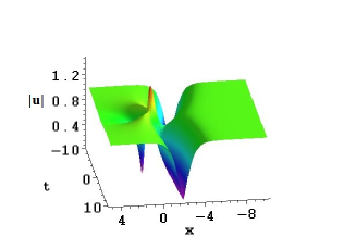
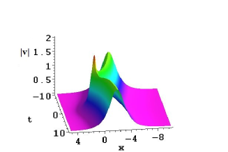
$(\rm{a})$                                            $(\rm{b})$

Fig. 1: Evolution plot of the dark-bright-rogue wave in coupled Hirota equations with the parameters chosen by $\epsilon=1/100,\alpha=10,d_{1}=1,d_{2}=0$. (a) a dark soliton merge with a rogue wave in $u$ component; (b) a bright soliton merge with a rogue wave in $v$ component.

(ii) $\alpha\neq 0$, $d_{1}\neq 0$ and $d_{2}=0$. In this case, the dark-bright-rogue wave solution can be generated. Fig. 1 shows a dark-bright soliton together with a rogue wave, and Figs. 2 and 3 describe the explicit collision processes between a dark soliton and a rogue wave, a bright soliton and a rogue wave, respectively. We see that in Figs. 2 and 3, a dark soliton and a bright soliton are propagating in the positive direction of $x$-axis, while at the time of $t=0$, a rogue wave suddenly appears from nowhere, and these two different types of waves impact together with each other. Next, the rogue wave soon disappears in the same abrupt way, and the solitons continue going ahead without any changing of their amplitudes and velocities after the collision. The whole interactional process can be seen as elastic. Moreover, by decreasing the value of $\alpha$, the dark-bright soliton and the rogue wave separate. We notice that in Fig. 4(a), a dark soliton and a rogue wave emerge on the distribution of the spacial-temporal structure, and the maximum amplitude of the rogue wave is 3. Nevertheless, when the bright soliton and the rogue wave divide, it is shown that the rogue wave can not be easily identified, see Fig. 4(b). The phenomenon can be easily explained, for the amplitude of a rogue wave depend on that of its background wave, and at this time the amplitude of the background wave in $v$ component is zero.

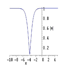
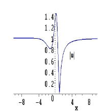
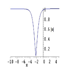
$(\rm{a})$                                    $(\rm{b})$                                    $(\rm{c})$

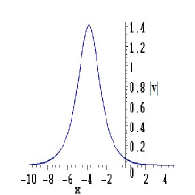
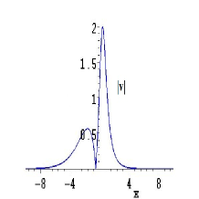
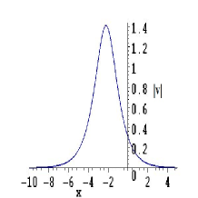
Fig. 2: Plane evolution plot of the interactional process between a right-going dark soliton and a rogue wave in Fig. 1(a) at: (a) $t=-20$; (b) $t=0$; (c) $t=20$. The collision process is elastic, the amplitude and velocity of the dark soliton are unchanged after the collision.

$(\rm{a})$                                    $(\rm{b})$                                    $(\rm{c})$

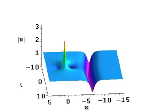
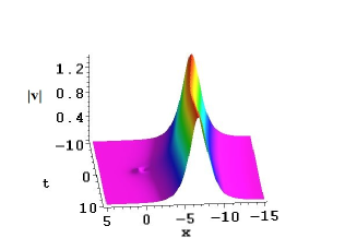
Fig. 3: Plane evolution plot of the interactional process between a right-going bright soliton and a rogue wave in Fig. 1(b) at: (a) $t=-20$; (b) $t=0$; (c) $t=20$. The collision process is elastic, the amplitude and velocity of the bright soliton are unchanged after the collision.

$(\rm{a})$                                            $(\rm{b})$

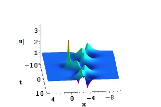
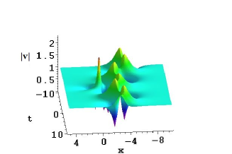
Fig. 4: Evolution plot of the dark-bright-rogue wave in coupled Hirota equations with the parameters chosen by $\epsilon=1/100,\alpha=1/10,d_{1}=1,d_{2}=0$. (a) the dark soliton and the rogue wave separate in $u$ component; (b) the bright soliton and the rogue wave separate in $v$ component. The rogue wave in $v$ component is difficult to be seen for its zero-amplitude background wave.

$(\rm{a})$                                            $(\rm{b})$

Fig. 5: Evolution plot of the breather-rogue wave in coupled Hirota equations with the parameters chosen by $\epsilon=1/100,\alpha=1,d_{1}=1,d_{2}=1$. (a) an Akhmediev breather merge with a rogue wave in $u$ component; (b) an Akhmediev breather merge with a rogue wave in $v$ component.

(iii) $\alpha\neq 0$, $d_{1}\neq 0$ and $d_{2}\neq 0$. At this point, the interactional solution between an Akhmediev breather and a rogue wave can be given, see Figs. 5 and 6. We observe that by increasing the value of $\alpha$, the Akhmediev breather and the rogue wave merge, see Fig. 5. While by decreasing the value of $\alpha$, the Akhmediev breather and the rogue wave separate, see Fig. 6.

Next, considering the following limit

$$\lim\limits_{f\rightarrow 0}\frac{\displaystyle T[1]|_{\zeta=8{\rm i}\epsilon\sqrt{d_{1}^{2}+d_{2}^{2}}(1+f^{2})}\Phi_{1}}{\displaystyle f^{2}}=\lim\limits_{f\rightarrow 0}\frac{\displaystyle(8{\rm i}\epsilon\sqrt{d_{1}^{2}+d_{2}^{2}}f^{2}+T_{1}[1])\Phi_{1}}{\displaystyle f^{2}}=8{\rm i}\epsilon\sqrt{d_{1}^{2}+d_{2}^{2}}\Phi_{1}^{[0]}+T_{1}[1]\Phi_{1}^{[1]}\equiv\Phi_{1}[1],$$ (31)

where $\Phi_{1}^{[1]}=\displaystyle\frac{1}{2}\frac{\partial^{2}}{\partial f^{2}}|_{f=0}\Phi_{1}$, we get a special solution of the Lax pair (3) and (4) with $u[1]$, $v[1]$ and $\zeta=\zeta_{1}=8{\rm i}\epsilon\sqrt{d_{1}^{2}+d_{2}^{2}}$. By making use of (18) and (19), the explicit second-order localized wave solution can be obtained. Here, we only give the explicit expressions of $u[2]$ and $v[2]$ in the simplest case of $\alpha=0$. For the case of $\alpha\neq 0$, we omit presenting since the expressions are rather cumbersome to write them down here, although it is not difficult to verify the validity of the solution by putting them back into Eqs. (1) and (2) using Maple.

(i) $\alpha=0$. By taking $d_{1}=1,d_{2}=3/2$, we calculate that

$$u[2]_{rw}=\exp({\displaystyle\frac{13}{4}{\rm i}t})(1+\frac{F_{2}+{\rm i}H_{2}}{D_{2}}),\ v[2]_{rw}=\frac{3}{2}\exp({\displaystyle\frac{13}{4}{\rm i}t})(1+\frac{F_{2}+{\rm i}H_{2}}{D_{2}}),$$ (32)

where

$$\begin{array}[]{l}F_{2}=-129792\epsilon^{2}x^{4}+10123776\epsilon^{3}tx^{3}-(296120448\epsilon^{4}t^{2}+2530944\epsilon^{2}t^{2}+59904\epsilon^{2})x^{2}+(3849565824\epsilon^{5}t^{3}\\ ~{}~{}~{}~{}~{}+98706816\epsilon^{3}t^{3}+5451264\epsilon^{3}t+7488\epsilon m_{1})x-24\epsilon(781943058\epsilon^{5}+285610\epsilon+40099644\epsilon^{3})t^{4}\\ ~{}~{}~{}~{}~{}-24\epsilon(3480048\epsilon^{3}+24336\epsilon)t^{2}+24\epsilon(156\sqrt{13}n_{1}-6084\epsilon m_{1})t+2304\epsilon^{2},\\ G_{2}=-843648t\epsilon^{2}x^{4}+65804544\epsilon^{3}t^{2}x^{3}-(1924782912\epsilon^{4}t^{3}-389376\epsilon^{2}t+3744n_{1}\epsilon\sqrt{13}+5483712\epsilon^{2}t^{3})x^{2}\\ ~{}~{}~{}~{}~{}+(25022177856\epsilon^{5}t^{4}+213864768\epsilon^{3}t^{4}+5061888\epsilon^{3}t^{2}+48672\epsilon m_{1}t+146016\sqrt{13}\epsilon^{2}n_{1}t)x-24\epsilon(371293\epsilon\\ ~{}~{}~{}~{}~{}+5082629877\epsilon^{5}+86882562\epsilon^{3})t^{5}-24\epsilon(17576\epsilon+10281960\epsilon^{3})t^{3}+24\epsilon(507\sqrt{13}n_{1}-59319\sqrt{13}\epsilon^{2}n_{1}\\ ~{}~{}~{}~{}~{}-39546\epsilon m_{1})t^{2}+74880\epsilon^{2}t-288\sqrt{13}\epsilon n_{1},\\ D_{2}=140608\epsilon^{2}x^{6}-16451136\epsilon^{3}tx^{5}+((801992880\epsilon^{4}+1370928\epsilon^{2})t^{2}+32448\epsilon^{2})x^{4}-((106932384\epsilon^{3}\\ ~{}~{}~{}~{}~{}+20851814880\epsilon^{5})t^{3}-843648\epsilon^{3}t-8112\epsilon m_{1})x^{3}+((304957792620\epsilon^{6}+4455516\epsilon^{2}+3127772232\epsilon^{4})t^{4}\\ ~{}~{}~{}~{}~{}-(123383520\epsilon^{4}+632736\epsilon^{2})t^{2}+(12168\sqrt{13}\epsilon n_{1}-474552\epsilon^{2}m_{1})t+22464\epsilon^{2})x^{2}-((173765124\epsilon^{3}\\ ~{}~{}~{}~{}~{}+40661039016\epsilon^{5}+2378670782436\epsilon^{7})t^{5}-(2887174368\epsilon^{5}-8225568\epsilon^{3})t^{3}-(9253764\epsilon^{3}m_{1}-79092\epsilon m_{1}\\ ~{}~{}~{}~{}~{}-474552\sqrt{13}\epsilon^{2}n_{1})t^{2}+1654848\epsilon^{3}t+1872\epsilon m_{1})x+(4826809\epsilon^{2}+7730680042917\epsilon^{8}+198222565203\epsilon^{6}\\ ~{}~{}~{}~{}~{}+1694209959\epsilon^{4})t^{6}+(400996440\epsilon^{4}+3084588\epsilon^{2}-20330519508\epsilon^{6})t^{4}+(4626882\sqrt{13}\epsilon^{3}n_{1}\\ ~{}~{}~{}~{}~{}-13182\sqrt{13}\epsilon n_{1}+1542294\epsilon^{2}m_{1}-60149466\epsilon^{4}m_{1})t^{3}+(43975152\epsilon^{4}+267696\epsilon^{2})t^{2}+(133848\epsilon^{2}m_{1}\\ ~{}~{}~{}~{}~{}-2808\sqrt{13}\epsilon n_{1})t+117m_{1}^{2}+117n_{1}^{2}+576\epsilon^{2}.\end{array}$$

Then $u[2]_{rw}$ is merely proportional to $v[2]_{rw}$ with the radio of $2/3$, the maximum value of them with $m_{1}=0$ and $n_{1}=0$ are five times more than their each average crest. Thus, the above solution is the vector generalization of the second-order rogue wave solution to the decoupled Hirota equation.

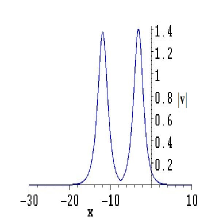
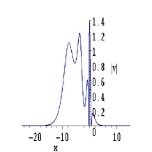
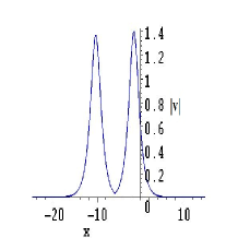
$(\rm{a})$                                    $(\rm{b})$                                    $(\rm{c})$

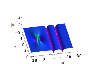
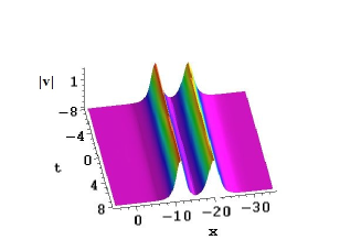
Fig. 9: Plane evolution plot of the interactional process between two bright solitons and a fundamental second-order rogue wave in Figs. 7(b) at: (a) $t=-20$; (b) $t=0$; (c) $t=20$. The collision process is elastic, the amplitude and velocity of the bright solitons are unchanged after the collision.

$(\rm{a})$                                            $(\rm{b})$

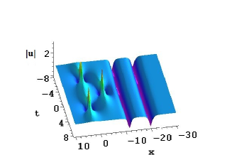
Fig. 10: Evolution plot of the second-order dark-bright-rogue wave in coupled Hirota equations with the parameters chosen by $\epsilon=1/100,\alpha=1/10000,d_{1}=1,d_{2}=0,m_{1}=0,n_{1}=0$. (a) two dark solitons and a fundamental second-order rogue wave separate in $u$ component; (b) two bright solitons and a fundamental second-order rogue wave separate in $v$ component. The rogue wave in $v$ component is difficult to be seen for its zero-amplitude background wave.

$(\rm{a})$                                            $(\rm{b})$

Fig. 11: Evolution plot of the second-order dark-bright-rogue wave in coupled Hirota equations with the parameters chosen by $\epsilon=1/100,\alpha=1/10000,d_{1}=1,d_{2}=0,m_{1}=10,n_{1}=0$. (a) two dark solitons together with a second-order rogue wave of triangular pattern in $u$ component; (b) two bright solitons together with a second-order rogue wave of triangular pattern in $v$ component. The rogue waves in $v$ component are difficult to be seen for its zero-amplitude background wave.

(ii) $\alpha\neq 0$, $d_{1}\neq 0$ and $d_{2}=0$. Hence we arrive at the interactional solution between two dark-bright solitons and a second-order rogue wave. Fig. 7(a) displays two dark solitons together with a fundamental second-order rogue wave, Fig. 7(b) shows two bright solitons coexist with a fundamental second-order rogue wave. The explicit collision processes are exhibited in Figs. 8 and 9. It is shown that the interactional process is also elastic, the amplitudes and velocities of the two dark and bright solitons remain unchanged after the collision. When by decreasing the value of $\alpha$, the two dark-bright solitons and the fundamental second-order rogue wave separate, see Fig. 10. At this moment, when the two bright solitons and the second-order rogue wave divide, the second-order rogue wave in $v$ component are also unobservable for the same reason as the first-order case. When setting $s_{1}\neq 0$, the fundamental second-order rogue wave can split into three first-order rogue waves, see Fig. 11.

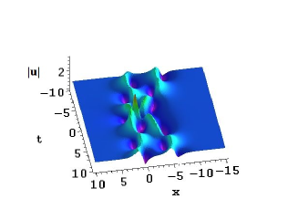
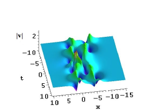
$(\rm{a})$                                            $(\rm{b})$

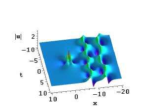
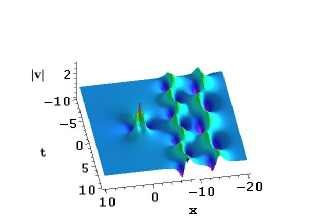
Fig. 12: Evolution plot of the second-order breather-rogue wave in coupled Hirota equations with the parameters chosen by $\epsilon=1/100,\alpha=10,d_{1}=1,d_{2}=1,m_{1}=0,n_{1}=0$. (a) two Akhmediev breathers merge with a fundamental second-order rogue wave in $u$ component; (b) two Akhmediev breathers merge with a fundamental second-order rogue wave in $v$ component.

$(\rm{a})$                                            $(\rm{b})$

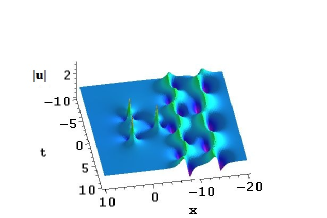
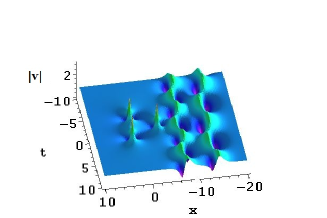
Fig. 13: Evolution plot of the second-order breather-rogue wave in coupled Hirota equations with the parameters chosen by $\epsilon=1/100,\alpha=1/10000,d_{1}=1,d_{2}=1,m_{1}=0,n_{1}=0$. (a) two parallel Akhmediev breathers and a fundamental second-order rogue wave separate in $u$ component; (b) two parallel Akhmediev breathers and a fundamental second-order rogue wave separate in $v$ component.

$(\rm{a})$                                            $(\rm{b})$

Fig. 14: Evolution plot of the second-order breather-rogue wave in coupled Hirota equations with the parameters chosen by $\epsilon=1/100,\alpha=1/10000,d_{1}=1,d_{2}=1,m_{1}=10,n_{1}=0$. (a) two parallel Akhmediev breathers and a second-order rogue wave of triangular pattern separate in $u$ component; (b) two parallel Akhmediev breathers and a second-order rogue wave of triangular pattern separate in $v$ component.

(iii) $\alpha\neq 0$, $d_{1}\neq 0$ and $d_{2}\neq 0$. Here, the interactional solutions between two Akhmediev breathers and a second-order rogue wave can be presented, see Figs. 12-14. We see that by increasing the value of $\alpha$, the two Akhmediev breathers and the second-order rogue wave merge, see Fig. 12. While by decreasing the value of $\alpha$, the two parallel Akhmediev breathers and the second-order rogue separate, see Fig. 13. Meanwhile, when taking $s_{1}\neq 0$, the fundamental second-order rogue wave can split into three first-order rogue waves, see Fig. 14.

4 Conclusion

In summary, we present some novel localized wave solutions of the coupled Hirota equations with high-order nonlinear effects like the third dispersion, self-steepening and inelastic Raman scattering terms. By using the Taylor series expansion coefficients of a special solution (27) to the Lax pair equations (3) and (4) with a periodic seed solution and a fixed spectral parameter, a generalized Darboux transformation of the coupled Hirota equations is constructed. As application, the interesting interactions between rogue waves and the other nonlinear waves such as dark-bright solitons and Akhmediev breathers in the coupled Hirota equations are illustrated through some figures. Several free parameters such as $\alpha$, $d_{i}~{}(i=1,2)$ and $s_{1}$ play an important part to affect the dynamic structures of the localized waves. (1) When $\alpha=0$, the first- and the second-order localized wave solutions are the vector generalization of the corresponding rogue wave solutions to the decoupled Hirota equation. (2) When $\alpha\neq 0$, $d_{1}\neq 0$ and $d_{2}=0$, the first- and the second-order dark-bright-rogue wave solutions are reached. (3) When $\alpha\neq 0$, $d_{1}\neq 0$ and $d_{2}\neq 0$, the first- and the second-order breather-rogue wave solutions are derived. Moreover, by increasing the value of $\alpha$, the rogue waves and the dark-bright solitons or breathers merge, by decreasing the value of $\alpha$ they separate, and by taking $s_{1}\neq 0$, the fundamental second-order rogue wave can split into three first-order rogue waves. Our results can be seen as the generalization of the work done by Baronio et al. [29] to the complex coupled system with high-order nonlinear terms.

Besides, on the one hand, continuing the generalized DT process, the more complicated localized wave solutions can be generated, which may possess more abundant striking dynamics. On the other hand, the interactions between rogue waves and cnoidal waves have recently been reported in the NLS equation [49], there are many possibilities to be observed in the coupled Hirota equations. Both of them are interesting and we will investigate in the future paper. The results in the present paper further reveal the intriguing dynamic distributions of localized waves in the coupled Hirota equations with high-order nonlinear terms, and we hope our results can be verified in real experiments in the future.

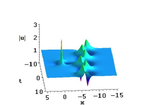
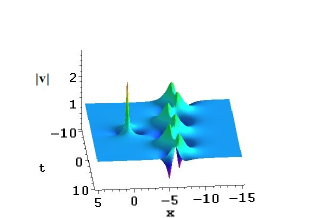
$(\rm{a})$                                            $(\rm{b})$

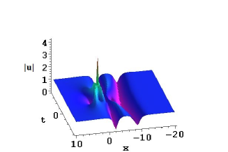
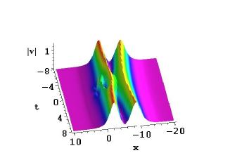
Fig. 6: Evolution plot of the breather-rogue wave in coupled Hirota equations with the parameters chosen by $\epsilon=1/100,\alpha=1/100,d_{1}=1,d_{2}=1$. (a) the Akhmediev breather and the rogue wave separate in $u$ component; (b) the Akhmediev breather and the rogue wave separate in $v$ component.

$(\rm{a})$                                            $(\rm{b})$

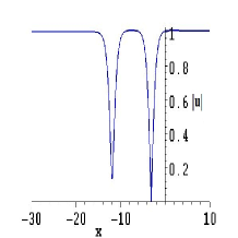
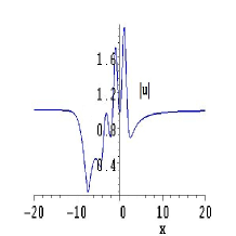
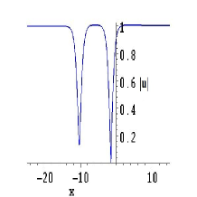
Fig. 7: Evolution plot of the second-order dark-bright-rogue wave in coupled Hirota equations with the parameters chosen by $\epsilon=1/100,\alpha=1,d_{1}=1,d_{2}=0,m_{1}=0,n_{1}=0$. (a) two dark solitons merge with a fundamental second-order rogue wave in $u$ component; (b) two bright solitons merge with a fundamental second-order rogue wave in $v$ component.

$(\rm{a})$                                    $(\rm{b})$                                    $(\rm{c})$

Fig. 8: Plane evolution plot of the interactional process between two dark solitons and a fundamental second-order rogue wave in Figs. 7(a) at: (a) $t=-20$; (b) $t=1$; (c) $t=20$. The collision process is elastic, the amplitude and velocity of the dark solitons are unchanged after the collision.

References