An ESPResSo implementation of elastic objects immersed in a fluid

Abstract

We review the lattice-Boltzmann (LB) method coupled with the immersed boundary (IB) method for the description of combined flow of particulate suspensions with immersed elastic objects. We describe the implementation of the combined LB-IB method into the open-source package ESPResSo. We present easy-to-use structures used to model a closed object in a simulation package, the definition of its elastic properties, and the interaction between the fluid and the immersed object. We also present the test cases with short examples of the code explaining the functionality of the new package.

FRAMEWORK FEATURES
Feature	OIF command example and options
Templates	if_create_template \ \ \ \verb template-id \ 0 \\ \hs ge metry	odes-file \ ".dat”, riangles-file \ ".dat”
elastic properties	s \ 0.1, \verb b  0.03, al \ 0.1, \verb ag  0.4, v \ 1.0 \\ \end{tabular} \vspace{0.3cm} \noindent \begin{tabular}{p{3.2cm}p{11.5cm}} {\bf Objects} & \verb oif_add_object \ \ \ \verb object-id \ 0 \\ \hs source template & \hs \verb template-id \ 1 \\ \hs position, rotation & \hs \verb origin \ 10 8 13, \hs \verb rotate \ $\pi/2$ \ 0 \ $\pi/4$ \\ \end{tabular} \vspace{0.3cm} \noindent \begin{tabular}{p{3.2cm}p{11.5cm}} {\bf Properties} & \verb oif_object_set \ \ \ \verb object-id \ 0 \\ \hs position & \hs \verb origin \ 10 8 13 \\ \hs external forces & \hs \verb force \ 3 0 0 \\ \hs deformation & \hs \verb mesh-nodes \ "deformed.dat" \\ \end{tabular} \vspace{0.3cm} \noindent \begin{tabular}{p{3.2cm}p{11.5cm}} {\bf Output} & \verb oif_object_output \ \ \ \verb object-id \ 0 \\ \hs vt visualization	tk-pos \ "pos.tk”
deformation	esh-nodes \ "defored.dat”

Mesh	if_check_mesh \\ \hs mesh files & \hs \verb n des-file  ”n.dat”, riangles-file \ ".dat”
mesh analysis	rientatin
mesh repair	epai  ”r.dat”

Other
initialization	if_init \ \\ \hs inf rmation	if_inf

1 Introduction

The simulations of flow with immersed objects are a key technique for analysis in numerous areas. One can simulate the propulsion of bacteria [maniyeri2012], another application is the analysis of fish-like behavior [gilmanov2005]. Our current research is motivated by biomedical applications for which simulation of blood on the level of blood cells immersed in a fluidic blood plasma is crucial (Fig. 1). These applications require understanding of processes depending on individual behavior of particular cells. Among others, we speak about microfluidic devices aimed for filtering of circulating tumor cells from blood [chen2012].

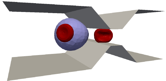
(a)

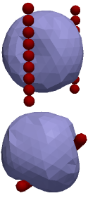
(b)

Figure 1: Elastic objects in biomedical applications a) Simulation of blood flow through tunable magneto-active polymer channel [gusenbauer2013] b) Circulating tumor cell captured in magnetic bead trap (side and top view) [gusenbauer2012]

We utilize the lattice-Boltzmann (LB) method for the description of the fluid dynamics and the immersed boundary (IB) method for the description of the immersed objects. The coupling of both methods provides an accurate description of the complete fluid-structure interactions.

The lattice-Boltzmann method is a powerful technique enabling fast and accurate computation of the fluid flow in complex structures [guo2002, kutay2006, geller2006]. In its nature, it is suitable for parallelization, performing very well in the benchmark examples [kandhai1998, satofuka1999, williams2009]. The LB method describes the flow dynamics by giving information about the fluid velocity and pressure in each space-time discretization point of the computational domain.

The immersed boundary (IB) method is based on the discretization of the boundary of the immersed object. The method was first introduced by Charles S. Peskin in 1972 [peskin1972]. The advantage of the method lies in its ability to capture the changes in the shape of the object without re-meshing and adaptive refinement of the underlying meshes. This is a crucial advantage for the simulation of moving boundaries.

2 Method

The ESPResSo package is aimed for soft-matter simulations. Originally, it was intended for simulations of different chemical systems where molecules and atoms are involved. These atoms are modeled as particles with their own mass. User defines bonds and potentials that generate forces between the particles. Consequently, particles move in the space subject to these forces and numerous other constraints.

In later releases of ESPResSo, the LB method was implemented to simulate soft-matter systems immersed in fluid. However, the package had no concept of a closed object. All the entities simulated in ESPResSo were open, tree-like structures without inner volume and surface. Our idea was to extend the functionality of ESPResSo by introducing closed objects with their own particle management in order to simulate elastic objects immersed in a fluid.

In this section, we first briefly describe the LB method as it was implemented in the original version of ESPResSo. Then we describe the IB method that we have implemented.

Lattice Boltzmann method: This method is based on fictive particles. These particles perform consecutive propagations and collisions over a fixed discrete lattice. Consider a lattice placed over the three-dimensional domain and consisting of identical cubic cells. This lattice creates an Eulerian grid which is fixed during the entire simulation. The variable of interest in the LB method is $n_{i}(x,t)$ which is the particle density function for the lattice point $x$, discrete velocity vector $e_{i}$, and time $t$. We use the D3Q19 version of the LB method (three dimensions with 19 discrete directions $e_{i}$, so $i=0,...,18$). The governing equations in the presence of external forces, are

$$\underbrace{\vphantom{\frac{1}{\tau}}n_{i}(x+e_{i}\delta_{t},t+\delta_{t})=n_{i}(x,t)}_{propagation}-\underbrace{\vphantom{\frac{1}{\tau}}\Delta_{i}(\textbf{n}(x,t))}_{collision}+\underbrace{\vphantom{\frac{1}{\tau}}f_{i}(x,t)}_{externalforces}$$ (1)

where $\delta_{t}$ is the time step and $\Delta_{i}$ denotes the collision operator that accounts for the difference between pre- and post-collision states and satisfies the constraints of mass and momentum conservation. $f_{i}$ is the external force exerted on the fluid. We refer to [Ahlrichs1998] and [dunweg2008] for details on the LBM. The macroscopic quantities such as velocity $u$ and density $\rho$ are evaluated from

$$\rho(x,t)=\sum_{i}n_{i}(x,t)\qquad\mathrm{and}\qquad\rho(x,t)u=\sum_{i}n_{i}(x,t)e_{i}.$$

Immersed Boundary method: This method is based on the discretization of object’s boundary. The boundary is covered by a set of IB points linked by triangular mesh, which is called Lagrangian mesh. The positions of IB points are not restricted to any lattice. To take the mechano-elastic properties of the immersed objects into account, geometrical entities in this mesh (edges, faces, angles between two faces, …) are used to model stretching, bending, stiffness, and other properties of the boundary. They define forces according to the current shape of the immersed object that are exerted on IB points. These forces cause motion of the IB points according to the Newton’s equation of motion

$$m\frac{d^{2}X_{j}}{dt^{2}}=F_{j}$$ (2)

where $m$ is the mass of the IB point, $X_{j}$ is the position and $F_{j}$ is the force exerted on the particular IB point $j$. The source of $F_{j}$ is either from the above mentioned elasto-mechanical properties of the immersed object, or from the fluid-structure interaction.

Equations (1) and (2) describe two different model components on two different meshes: the motion of the fluid and the motion of the immersed objects. For coupling, ESPResSo uses an approach from [Ahlrichs1998] with a drag force that is exerted on a sphere moving in the fluid. Analogous to the Stokes formula for the sphere in a viscous fluid, we assume the force exerted by the fluid on one IB point to be proportional to the difference of the velocity $v$ of the IB point and the fluid velocity $u$ at the same position,

$$F_{j}=\xi(v-u).$$ (3)

Here $\xi$ is a proportionality coefficient which we will refer to as the friction coefficient. In the previous expression, the velocities $v$ and $u$ are computed at the same spatial location, whereas we posses $u$ in fixed Eulerian grid points and $v$ in moving Lagrangian IB points. Therefore, for computation of $u$ at the IB point, we use linear interpolation of the $u$ values from nearby fixed grid points.

There is also an opposite effect: not only fluid acts on the IB point, but also the IB point acts on the fluid. Therefore, the opposite force $-F_{j}$ needs to be transferred back to the fluid. $F_{j}$ from the location of the IB point is distributed to the nearest grid points. Distribution is inversely proportional to the cuboidal volumes with opposite corners being the IB point and the grid point [Ahlrichs1998].

3 Object-in-fluid framework

We implement an object-in-fluid (OIF) framework into ESPResSo that allows the use of objects with inner volume, for example blood cells, magnetic beads, capsules and so on. We use LB-IB method where IB points from the triangulation are identified with ESPResSo particles. The edges of the triangular mesh are identified as bonds in ESPResSo. Bonds generate elastic forces that keep the shape of the object. The movement of the object is achieved by applying calculated forces to the IB points.

The immersed objects are composed of a membrane encapsulating the fluid inside the object. For now, the inside fluid must have the same density and viscosity as the outside fluid.

The original ESPResSo works with particles that can be defined by a single art \ command executed for each article. Particles are virtually connected with bonds executing nter \ and \verb part \ \verb bond \ commands. To create a mesh, e.g. a trangular mesh with 300 mesh nodes covering a sphere, one needs to execute a series of commands analyzing the mesh, computing hundreds of edge lengths, all angles between triangles, etc. Afterwards, more than thousand commands must be executed to add the particles and define the bonds. In the OIF framework we enable the automatization of this process with numerous features.

The OIF framework works in two steps. First, one needs to create a template, then one can add actual objects. The template has its own elastic properties and shape. Templates are not real objects, they only keep information about the objects to be created. After a template (or several templates) is created, one can add actual objects to the simulation by specifying the template from which the object takes its geometry and elastic properties, the location and, optionally, the rotation of the object.

During the simulation, one can analyze the objects by printing their physical properties. Also, different quantities characterizing the objects can be set.

Further functionality includes analysis of the mesh files, output for the VTK visualization using a standalone visualization software, e.g. ParaView [paraview]. Detailed description of all currently implemented features of the OIF framework is in Section 5. However, the OIF framework is a lively project that is being extended on regular base. Therefore for up-to-date documentation on the latest developments we recommend the ESPResSo documentation [espressoDocumentation].

4 Elastic interactions

The generic implementation of bonded interactions in ESPResSo is described in detail in [Limbach2006, Arnold2013]. Bonded interactions are always defined between two, three or sometimes four points. They generate forces that are exerted on each IB point. These forces must be evaluated at a certain point of the integration algorithm. At that moment, with given positions of the IB points, the forces for each specific interaction can be calculated and added to the IB points.

Parameters: There are several parameters involved in this model. All of them should be calibrated with respect to the application.

Mass of the particles: Every particle has its mass that influences the dynamics. Its default value is one, however it can be changed when adding the object into simulation with if_add_bject  ass \ comand.

Friction coefficient $\xi$: The parameter describing the strength of fluid-particle interaction is the riction \ parameter rom the original ESPResSo command bfuid , see (3).

Parameters of elastic moduli: Elastic behavior can be described by five different elastic moduli: stretching, bending, local and global area preservation and volume preservation. Each of them has its own scaling parameter: s, \verb b, al, \verb ag, v. \ %Their mathematical formulations have been taen from [dupin2007].

The mass of the particles and the friction coefficient can be calibrated using the known analytical values of the drag coefficients for ellipsoidal objects. More details about the calibration is given in [cimrak11a].

The elastic parameters depend on the way how the physical properties are modeled. For each physical property there are always numerous approaches how to model that particular property. As a very simple example let us discuss the local area conservation. Assume an elastic object has a relaxed shape, in which this objects remains unless external forces are applied. In the relaxed shape, each local part of the surface has its area. The general idea is that once the local part of the object’s surface has a larger area than in the relaxed state then this part must be shrunk. If the current area is smaller than that in the relaxed shape, the surface must be expanded.

To implement this general idea we show two different approaches. Both approaches first compute the magnitude of the force that will be applied to each vertex of the triangles in the mesh. This magnitude is proportional to the difference between the current area of the triangle and the area in the relaxed shape. The directions of the forces however differ in the two approaches. First approach puts the forces in the direction from the vertex to the centroid of the triangle. The second approach applies the forces in the vertices in the direction of the respective altitudes of the triangle. Both approaches follow the main idea, however the actual effect on the triangle is different.

In the current version of the OIF framework, we work with the elastic models taken from [Dao2003]. More details about the mechanical and biological aspects specifically for red blood cells are presented in the cited work. The proper calibration to fit the experimental data has been performed in [cimrak11a, Cimrak2013].

However, we are aware of the different approaches. Authors in [Fedosov2010a, Fedosov2010b, Odenthal2013] use the energy approach where the forces are derived from the energy contributions rather than defined explicitly as in [Dao2003]. The OIF framework is flexible enough to implement any method based on the application of forces to the nodes in the triangular mesh.

The following interactions are implemented in order to mimic the mechanics of elastic or rigid objects immersed in the LB fluid flow. They are all based on the fact that an elastic object without any external forces has a relaxed shape. The object always tends to recover this relaxed shape. Once this shape is deformed, elastic forces act on the boundary of the object, trying to return it to its relaxed state. So for example, all edges of the triangulation in the relaxed shape have a reference length which we call relaxed length. Similarly, there is a relaxed angle between two incident triangles in the mesh, a relaxed area of each triangle in the mesh and so on.

The elastic forces have specific expressions for each elastic modulus. Their mathematical formulations have been taken from [Dupin2007].

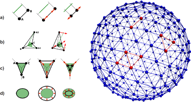
Figure 2: Elastic sphere model in ESPResSo:
a) stretching force, b) bending force, c) local area force, d) volume force/global area force

Stretching force

This type of interaction is available for closed 3D immersed objects as well as for 2D sheet flowing in the 3D flow.

It forces each triangulation edge to adjust towards its relaxed length. For each edge of the mesh, $L$ is the current length of the edge. By $L^{0}$ we denote the relaxed length. In the case of $L=L^{0}$ no forces are added. $\Delta L=L-L^{0}$ denotes the deviation from the relaxed length. The stretching force acting on edge endpoints is computed using

$$F_{\mathrm{s}}=k_{\mathrm{s}}\kappa(\lambda)\frac{\Delta L}{L^{0}}n.$$ (4)

Here, $\mathrm{\mathit{n}}$ is the unit vector pointing from the one edge endpoint to the other, $k_{\mathrm{s}}$ is the stretching constant, $\lambda=L/L^{0}$, and $\kappa$ is a nonlinear function that resembles neo-Hookean behavior

$$\kappa(\lambda)=\frac{\lambda^{0.5}+\lambda^{-2.5}}{\lambda+\lambda^{-3}}.$$ (5)

For linear behavior of the stretching force we simply have $\kappa=1$. The stretching force acts between two particles and is symmetric (Figure 2a).

Bending force

Beside the stretching force, the tendency of an elastic object to maintain the relaxed shape is governed also by prescribing the preferred angles between two incident triangles of the mesh. This type of interaction is available for closed 3D immersed objects, as well as for 2D sheet flowing in the 3D flow.

The angle between two triangles in the resting shape is denoted by $\theta^{0}$. For closed immersed objects, one always has to set the inner angle. The deviation of this angle $\Delta\theta=\theta-\theta^{0}$ is computed and defines the bending force for each triangle.

$$F_{\mathrm{b}}=k_{\mathrm{b}}\frac{\Delta\theta}{\theta^{0}}n$$ (6)

Here, $n$ is the unit normal vector to the triangle and $k_{\mathrm{b}}$ is the bending constant. The force $F_{\mathrm{b}}$ is assigned to the two vertices not belonging to the common edge. The opposite force divided by two is assigned to the two vertices lying on the common edge (Figure 2b).

Unlike the stretching force, the bending force is strictly asymmetric. For more details, see the ESPResSo documentation [espressoDocumentation]. Notice, that concave objects can be defined as well. If $\theta_{0}$ is larger than $\pi$, then the inner angle is concave.

Local area conservation

This interaction conserves the area of the triangles in the triangulation. This type of interaction is available for closed 3D immersed objects, as well as for 2D sheet flowing in the 3D flow.

The deviation of the triangle surface $S$ is computed from the triangle surface in the resting shape $\Delta S=S-S^{0}$. The area constraint assigns the following shrinking/expanding force to every vertex

$$F_{\mathrm{al}}=-k_{\mathrm{al}}\frac{\Delta S}{S}w$$ (7)

where $k_{\mathrm{al}}$ is the area constraint coefficient, and $w$ is the unit vector pointing from the centroid of triangle to the vertex. Similarly, analogical forces are assigned to other vertices of the triangle (Figure 2c). This interaction is symmetric.

Global area conservation

This type of interaction is available for closed 3D immersed objects, as well as for 2D sheet flowing in the 3D flow.

The conservation of local area is sometimes too restrictive. The current surface of the whole immersed object is denoted by $\mathrm{\mathit{S_{g}}}$, the surface in the relaxed shape by $\mathrm{\mathit{S_{g}^{0}}}$ and $\Delta\mathrm{\mathit{S_{g}}}=\mathrm{\mathit{S_{g}}}-\mathrm{\mathit{S_{g}^{0}}}$. The global area conservation force is then defined as

$$F_{\mathrm{ag}}=-k_{\mathrm{ag}}\frac{\Delta S_{g}}{S_{g}}w$$ (8)

The force $F_{\mathrm{ag}}$ is assigned to all vertices of the object (Figure 2d).

Unlike the previous three forces (and related bonds), this one is different from classical bonds in ESPResSo, because it requires an advance calculation on the scale of the whole immersed object - to get its total area. This calculation has been implemented to allow for proper area computation also in parallelized simulations when parts of the given object lie in different blocks of the decomposed domain. In particular, consider a case when the immersed object lies in several regions that belong to different computational nodes. To compute the surface of such immersed object, each computational node needs to compute partial surface of the corresponding part and send the information to master to gather the whole surface of the object. To implement this, at each surface computation, a message is broadcasted to all computational nodes that adds the partial surface of the object. After gathering the information from all nodes, we can compute the actual forces for the global area conservation.

Volume conservation

This type of interaction is available solely for closed 3D immersed objects.

The deviation of the object’s volume $V$ is computed from the volume in the resting shape $\Delta V=V-V^{0}$. For each triangle the following force is computed

$$F_{\mathrm{v}}=-k_{\mathrm{v}}\frac{\Delta V}{V^{0}}S\ n$$ (9)

where $S$ is the area of triangle, $n$ is the normal unit vector of triangle’s plane, and $k_{\mathrm{v}}$ is the volume constraint coefficient. The volume of the immersed object is computed from

$$V=\sum_{triangles}S\ n\cdot h$$ (10)

where the sum is computed over all triangles of the mesh and $h$ is the unit vector from the centroid of triangle to a plane which does not cross the object. The force $F_{\mathrm{v}}$ is equally distributed to all three vertices (Figure 2d).

Similar to the computation of global area force, the volume force also requires a prior calculation on the scale of the whole object - to get the total volume. And again, it is implemented in such a way that partial volumes are added together in parallelized simulations when the object belongs to more than one block of decomposed domain.

Remark

The actual values of $k_{\mathrm{s}},k_{\mathrm{b}},k_{\mathrm{al}},k_{\mathrm{ag}},k_{\mathrm{v}}$ need to be calibrated for each type of the elastic object separately. They strongly depend on the physical values of elastic moduli. Their values can be determined e.g. from stretching experiments performed with red blood cells [Dao2003]. The stretching force expression (4) yields the sensitivity of $k_{\mathrm{s}}$ on the density of the triangular mesh. This dependence was elaborated in [Cimrak2013].

5 Implementation details and OIF command description

All commands and variables in the OIF framework start with prefix if_ . Syntax in the OIF framewrk follows the structure from ESPResSo. Each OIF command consists of command keyword followed by several option - arguments couples. The order of these couples is arbitrary. Some options of the commands are mandatory, some are optional. The options mostly have one or more arguments but there are also options without arguments.

The mandatory options are listed directly after the command keyword, the optional ones are listed inside brackets.

Initialization, general info

if_init \ & \\ \verb if_info

The first command initializes the OIF framework and must be used before any other OIF commands. It creates global variables used in the OIF framework. These variables are accessible on the Tcl level in ESPResSo, but for the ordinary user of the OIF framework it is not necessary to access them. The detailed description of the OIF variables is in the ESPResSo documentation.

The second command prints basic information about the current number of created templates and objects, etc.

Both commands are without options.

Template creation

if_create_template \ & \verb template-id \ \textit{tid} \ \verb ndes-file  nfile

riangles-file \ \extittfile  [tretch \ \textit{x sy sz]