One-Bit Compressed Sensing by Greedy Algorithms

Abstract

Sign truncated matching pursuit (STrMP) algorithm is presented in this paper. STrMP is a new greedy algorithm for the recovery of sparse signals from the sign measurement, which combines the principle of consistent reconstruction with orthogonal matching pursuit (OMP). The main part of STrMP is as concise as OMP and hence STrMP is simple to implement. In contrast to previous greedy algorithms for one-bit compressed sensing, STrMP only need to solve a convex and unconstraint subproblem at each iteration. Numerical experiments show that STrMP is fast and accurate for one-bit compressed sensing compared with other algorithms.

1 Introduction

Compressed sensing, or compressive sensing provides a new method of data sampling and reconstruction, which allows to recover sparse signals from much fewer measurements [5, 8]. Suppose that we have an unknown sparse signal $\hat{x}\in\mathbb{R}^{n}$ with $\|\hat{x}\|_{0}\leq s$ and $s\ll n$, where $\|\cdot\|_{0}$ denotes the number of nonzero components. We observe the signal as

$$b=A\hat{x},$$

where $A\in\mathbb{R}^{m\times n}$ is called measurement matrix, $b\in\mathbb{R}^{m}$ is the vector of measurements. Compressed sensing shows that only $m=O(s\log(n/s))$ measurements are sufficient for exact reconstruction of $\hat{x}$ under many settings for the measurement matrix $A$ [6, 8].

1.1 One-Bit Compressed Sensing

In compressed sensing, it is supposed that the measurements have infinite bit precision. However, in practice what we get is quantized measurements. In other words, the entries in the measurement vector $b$ must be mapped to a discrete set of values ${\mathcal{A}}$. There are much work about the recovery of the general signal from the quantized measurements [16]. In this paper, we focus on the case where ${\mathcal{A}}=\{-1,1\}$ with the mapping being done by the sign function. So we need to recover a $s$-sparse signal from $y:={\rm sign}(b)\in\{-1,1\}^{m}$. This problem is called one-bit compressed sensing, which was first introduced by Boufounos-Baraniuk [4]. In one-bit compressed sensing, we observe original signal as:

$$y={\rm sign}(A\hat{x}),$$

where $y\in\mathbb{R}^{m}$ with each element is sign of the corresponding element of $A\hat{x}$. That means we lost all magnitude information of $A\hat{x}$. Following [9], $x^{\sharp}\in{\mathbb{R}}^{n}$ is called a solution for one-bit compressed sensing corresponding to $A$ and $\hat{x}$ if it satisfies

• consistence, i.e. ${\rm sign}(Ax^{\sharp})={\rm sign}(A\hat{x})$,

• sparsity, i.e. $\|x^{\sharp}\|_{0}\leq\|{\hat{x}}\|_{0}$.

A simple observation is that ${\rm sign}(A\hat{x})={\rm sign}(Ac\hat{x})$ where $c>0$ is a scale. Thus the best one-bit compressed sensing can do is to recover $\hat{x}$ up to a positive scale. Therefore, we usually expect to recover original signal on the unit Euclidean sphere in practice.

1.2 Previous Work

A straightforward way to obtain a solution for one-bit compressed sensing is to solve the following program:

$$\min~{} \|x\|_{0}$$

s. t. $$y={\rm sign}(Ax)~{}\text{and}~{}\|x\|_{2}=1.$$ (1)

Since (1.2) is computational intractable, similar with compressed sensing, one can replace the $\ell_{0}$ norm by the more tractable $\ell_{1}$ norm and obtain that ( see [4, 13, 10])

$$\min~{} \|x\|_{1}$$

s. t. $$y={\rm sign}(Ax)~{}\text{and}~{}\|x\|_{2}=1.$$ (2)

Many algorithms have been proposed to solve (1.2). Particularly, in [10], Laska et. al. use the augmented Lagrangian optimization framework to design RSS algorithm with employing a restricted-step subroutine to solve a non-convex subproblem. Binary iterative hard thresholding (BIHT) and adaptive outlier pursuit (AOP) are introduced in [9] and [18], respectively. BIHT is the modification of iterative hard thresholding which is to solve compressed sensing problem (see [2]). AOP is a robust algorithm built on BIHT, and it is exactly BIHT when measurements are noise free. The numerical experiments in [18] show that AOP performs better than the previous existing algorithms in terms of the recovery performance. In [13], Plan and Vershynin replace the normalization constraint $\|x\|_{2}=1$ by $\|Ax\|_{1}=c_{0}$ and give an analysis of the following convex program

$$\min~{} \|x\|_{1}$$

s. t. $$y={\rm sign}(Ax)~{}\text{and}~{}\|Ax\|_{1}=c_{0},$$ (3)

where $c_{0}$ is a given positive constant.

Moreover, in compressed sensing, one develops many greedy algorithms to recover the sparse signals, such as OMP, CoSaMP, ROMP, OMMP and subspace pursuit etc (see [14, 11, 12, 7, 17] ). Motivated by these algorithms in compressed sensing, one also designs greedy algorithms for one-bit compressed sensing. Particulary, the matching sign pursuit (MSP) algorithm is presented in [3]. However, MSP suffers from time-consuming since it solves a non-convex sub-problem at each iteration. Naturally, one may be interested in designing more efficiently greedy-type algorithm for one-bit compressed sensing, which is also the start point of this project.

1.3 Our Contribution

The aim of this paper is to present the sign truncated matching pursuit (STrMP) algorithm, which is a new greedy algorithm to solve one-bit compressed sensing. In particular, motivated by [13], we replace the unit $\ell_{2}$-norm constraint by $\|Ax\|_{1}=c_{0}$ where $c_{0}$ is any fixed positive constant, and hence we consider the following optimization problem:

$$\min{} \|x\|_{0}$$ (4)

s. t. $$y={\rm sign}(Ax)~{}\text{and}~{}\|Ax\|_{1}=c_{0}.$$

A key step of STrMP algorithm is to use

$$j_{0}:=\mathop{\rm argmax}\limits_{i}\lvert A_{i}^{\top}y\rvert$$

to choose the first index $j_{0}$. We also prove that $j_{0}\in{\rm supp}({\hat{x}})$ with high probability provided $m=O(s\log n)$ and $A$ is a Gaussian matrix. If $j_{0}\in{\rm supp}({\hat{x}})$, we can remove the constraint $\|Ax\|_{1}=c_{0}$ and transform (4) to the program in the form of

$$\min{} \|z\|_{0}$$

s. t. $$y={\rm sign}(Pz+q),$$

where $P\in{\mathbb{R}}^{m\times(n-1)}$ and $q\in{\mathbb{R}}^{m}$, which is more convenient for designing greedy algorithms. We will introduce this and the algorithm in detail in section 2. STrMP algorithm overcomes the bottleneck of MSP that a non-convex problem need to be solved at each iteration. In fact, STrMP just need to solve a convex and unconstrained sub-problem at each iteration. Hence, numerical experiments show that STrMP outperforms previous existing algorithms in terms of speed. Moreover, the numerical experiments also show that the recovery performance of STrMP is better than that of MSP and is similar with that of BIHT or AOP. The last but not the least, beside the sparsity level, no parameter need to be adjusted in STrMP by the user.

1.4 Terminology and Organization

In the following of this paper, we denote by $A_{i}$ the $i$th column of matrix $A$, and $A_{ij}$ the $i$th row and $j$th column component of $A$. $e_{i}$ denotes the unit vector with the $i$th element is 1 and other elements are zero. For a vector $y\in\mathbb{R}^{m}$, ${\rm diag}(y)\in\mathbb{R}^{m\times m}$ denotes the diagonal matrix whose diagonal elements are corresponding elements of $y$. The symbol $[n]$ denotes the index set $\{1,2,\ldots,n\}$. For a subset $T\subset[n]$, $|T|$ denotes the number of elements in $T$. For a vector $x\in\mathbb{R}^{n}$ and a subset $T\subset[n]$, we use $x_{T}\in\mathbb{R}^{|T|}$ to denote the vector containing the entries of $x$ indexed by $T$. We use $x|_{T}\in\mathbb{R}^{n}$ to denote the vector whose entries indexed by $T$ are corresponding entries to $x$ and the entries indexed by $T^{c}$ are zero. For a matrix $A\in\mathbb{R}^{m\times n}$, $A_{T}\in\mathbb{R}^{m\times|T|}$ denotes a matrix which contains the columns of $A$ indexed by $T$. We define the sign truncated function as $(\cdot)_{-}:=\min\{\cdot,0\}$.

The rest of this paper is organized as follows. In section 2, we derive the STrMP algorithm, and also present the theorem which shows that one can choose the first index successfully with high probability provided $m=O(s\log n)$ and $A$ is a Gaussian matrix. The STrMP-$l_{1}$ algorithm, which is an adjustment of the STrMP algorithm is introduced in section 3. The numerical results, comparing with other algorithms, are illustrated in section 4. We conclude our results in section 5.

2 STrMP Algorithm

We derive the algorithm STrMP in this section. The algorithm is built on the following theorem, which shows that one can find a $x^{\sharp}$ which is a solution for one-bit compressed sensing by solving a program without the normalized constraint $\|Ax\|_{1}=c_{0}$.

Theorem 1:

Suppose that $j_{0}\in{\rm supp}(\hat{x})$ and $y^{\top}A_{j_{0}}\neq 0$ where $y={\rm sign}(A\hat{x})$. Suppose that $z^{\sharp}\in{\mathbb{R}}^{n-1}$ is a solution to

$$\min{} \|z\|_{0}$$ (5)

s. t. $$y={\rm sign}(Pz+q)$$

where $P=\left(I-\frac{A_{j_{0}}y^{\top}}{y^{\top}A_{j_{0}}}\right)A_{[n]\setminus\{j_{0}\}}$ and $q=\frac{c_{0}}{y^{\top}A_{j_{0}}}A_{j_{0}}$. Suppose that $x^{\sharp}$ is defined by

$$x^{\sharp}_{[n]\setminus\{j_{0}\}}:=z^{\sharp},\quad x^{\sharp}_{j_{0}}:=\frac{c_{0}-y^{\top}A_{[n]\setminus\{j_{0}\}}z^{\sharp}}{y^{\top}A_{j_{0}}}.$$ (6)

Then $\|Ax^{\sharp}\|_{1}=c_{0}$ and $x^{\sharp}\in{\mathbb{R}}^{n}$ is a solution for one-bit compressed sensing corresponding to $A$ and $\hat{x}$.

Based on Theorem 1, if knows an index $j_{0}\in{\rm supp}({\hat{x}})$ in advance, one can construct a solution for one-bit compressed sensing corresponding to $A$ and $\hat{x}$ by solving a program in the form of (5). STrMP algorithm uses

$$j_{0}=\mathop{\rm argmax}\limits_{i\in[n]}|A_{i}^{\top}y|$$

to choose the index $j_{0}$, and we also prove that $j_{0}\in{{\rm supp}}({\hat{x}})$ with high probability provided $m=O(s\log(n-s))$ and $A$ is a Gaussian matrix:

Theorem 2:

Let $\hat{x}$ be a $s$-sparse vector in ${\mathbb{R}}^{n}$. Let $A\in\mathbb{R}^{m\times n}$ be a random matrix with independent standard normal entries. Assume for some $\epsilon>0$

$$m\geq\frac{\pi}{2}s\left(\epsilon+\sqrt{\epsilon^{2}+2\log(n-s)}\right)^{2}.$$

Then

$$\mathop{\rm argmax}\limits_{i\in[n]}{|(A^{\top}{\rm sign}(A\hat{x}))_{i}|}\in{\rm supp}(\hat{x})$$

holds with probability at least $1-2e\cdot\exp(-c\epsilon^{2})$, where $c$ is an absolute constant.

We now focus on (5). A simple observation is that we can rewrite (5) as

$$\min{} \|z\|_{0}$$ (7)

s. t. $$Cz+d\geq 0,$$

where $C={\rm diag}(y)P$ and $d={\rm diag}(y)q$. We use greedy algorithms to find an approximate solution to (7). To state the algorithm, we recall that the sign truncated function $(\cdot)_{-}$ which is defined by $(\cdot)_{-}:=\min\{0,\cdot\}$. The algorithm begins with an initial support set $\Lambda^{0}=\emptyset$ and an estimate $z^{0}=0$. At the $k$th iteration, the algorithm computes the product of $C^{\top}$ and the sign truncated vector $(Cz^{k}+d)_{-}$ and form a proxy, where the truncated function $(\cdot)_{-}$ is applied component-wise to $Cz^{k}+d$. And use

$$j^{k}=\mathop{\rm argmax}\limits_{i}\lvert C_{i}^{\top}(Cz^{k}+d)_{-}\rvert$$

to choose a new index where $C_{i}^{\top}$ denotes transposition of $C_{i}$. Set $\Lambda^{k+1}:=\Lambda^{k}\cup\{j\}$. Next we solve a convex problem to enforce the consistence:

$${z}^{k+1}:=\mathop{\rm argmin}\limits_{z}\|(Cz+d)_{-}\|_{2}^{2}\qquad{\rm s.~{}t.}\qquad{\rm supp}(z)\subset\Lambda_{k+1},$$ (8)

which is essential unconstraint. We use two-point step size gradient method [1] to solve it and we introduce the algorithm in detail in Appendix B. We conclude above fact and formulate our algorithm in Algorithm 1.

Algorithm 1 The Sign Truncated Matching Pursuit (STrMP) Algorithm

0:  $A\in{\mathbb{R}}^{m\times n},~{}y\in\{-1,1\}^{m},~{}c_{0}>0,~{}s\in{\mathbb{Z}}^{+}$, residual tolerance $\varepsilon>0$ Initialization:  $\Lambda^{0}=\emptyset\subset[n]$, $z^{0}=0$, $k=0$

1:  Compute the first index $j_{0}=\mathop{\rm argmax}\limits_{i\in[n]}|(A^{\top}y)_{i}|$

2:  Set

$$C={\rm diag}(y)\left(I-\frac{A_{j_{0}}y^{\top}}{y^{\top}A_{j_{0}}}\right)A_{[n]\setminus\{j_{0}\}},~{}d=\frac{c_{0}}{y^{\top}A_{j_{0}}}{\rm diag}(y)A_{j_{0}}.$$

3:  while $\|(Cz^{k}+d)_{-}\|_{2}^{2}\geq\varepsilon$ and $k\leq s-1$ do

4:     Match: $h^{k}=C^{\top}(Cz^{k}+d)_{-}$

5:     Identify: $j^{k}=\mathop{\rm argmax}\limits_{i}|h^{k}_{i}|$

6:     Update: $\Lambda^{k+1}=\Lambda^{k}\cup\{j^{k}\}$,

7:         $\,\,{z^{k+1}}=\mathop{\rm argmin}\limits_{z\in{\mathbb{R}}^{n-1}}\|(Cz+d)_{-}\|_{2}^{2}~{}~{}{\rm s.t.}~{}z|_{({\Lambda}^{k+1})^{c}}=0$

8:     Increase iteration count: $k=k+1$

9:  end while

10:  Set $x^{k}_{[n]\setminus\{j_{0}\}}=z^{k},\quad x^{k}_{j_{0}}=\frac{c_{0}-y^{\top}A_{[n]\setminus\{j_{0}\}}z^{k}}{y^{\top}A_{j_{0}}}$

10:  $\frac{x^{k}}{\|x^{k}\|_{2}}$

Remark 1.

According to Theorem 1, the $x^{\sharp}$ defined by (6) is $s$-sparse and consistent. Then Theorem 2 in [9] shows that if $A$ is a Gaussian matrix, then

$$\|{x^{\sharp}}/{\|x^{\sharp}\|_{2}}-{\hat{x}}/{\|\hat{x}\|_{2}}\|_{2}=O\left(\frac{s}{m}\log\frac{mn}{s}\right),$$

holds with high probability.

Remark 2.

The code in Algorithm 1 describes a version of the STrMP algorithm. Similar to OMP, there are many adjustments of STrMP. Particularly, in the identify step, one can select many atoms per iteration instead of one atom, which is also helpful for improving the performance.

Remark 3.

A simple observation is that the output result of STrMP algorithm is independent of $c_{0}$ provided $c_{0}\gg\varepsilon$. In fact, for different positive $c_{0}$, the solution $z^{k+1}$ in the update step is the same up to a positive scale. And hence, in the identify step, STrMP algorithm chooses the same index $j$ even $c_{0}$ is different.

Remark 4.

Suppose that ${\hat{x}_{j}}=\pm\frac{1}{\sqrt{s}}$ holds for all $j\in{\rm supp}(\hat{x})$. The proof of Theorem 2 implies that, under the condition of Theorem 2, the $s$ indices corresponding to the largest magnitude entries in the vector $\lvert A^{\top}y\rvert$ are the support of $\hat{x}$ with high probability.

3 STrMP-$l_{1}$ Algorithm

In the update step of the STrMP algorithm, we use $\min_{z}\|(Cz+d)_{-}\|_{2}$ to enforce the consistence. Inspired by compressed sensing, we can replace $l_{2}$-norm by $l_{1}$-norm. Thus one may consider to solve following subproblem in the update step

$${z}^{k+1}:=\mathop{\rm argmin}\limits_{z}\|(Cz+d)_{-}\|_{1}\qquad{\rm s.~{}t.}\qquad{\rm supp}(z)\subset\Lambda_{k+1},$$ (9)

since $l_{1}$-norm is more effective to characterize the sparsity than $l_{2}$-norm. We apply quasi-Newton method to solve the subproblem (9). Correspondingly, in the match step, we compute

$$h^{k}=C^{\top}{\rm sign}(Cz^{k}+d)_{-},$$

which is exactly a subgradient of $\|(Cz+d)_{-}\|_{1}$ at $z^{k}$ (see [9]), and in identify step we set $j^{k}=\mathop{\rm argmax}\limits_{i}\lvert h_{i}^{k}\rvert$. Here, to state conveniently, we set ${\rm sign}(0)=0$. In the following of this paper, we denote this algorithm by STrMP-$l_{1}$.

4 Numerical Experiment

In this section, we make numerical experiments to compare the performance of STrMP with that of other existing methods as mentioned before, such as BIHT, MSP and RSS with showing that both STrMP and STrMP-$l_{1}$ are fast and accurate.

In our experiments, the measurement matrix $A\in\mathbb{R}^{m\times n}$ is generated by Gaussian random matrix. The original signal $\hat{x}\in\mathbb{R}^{n}$ is $s$-sparse, and its non-zero coefficients are drawn from standard normal distribution, and it is normalized to have unit $l_{2}$ norm. In all following experiments, we set $n=1000$. And in all following figures, the blue line with circles denotes STrMP, the black line with upward triangle denotes STrMP-$l_{1}$, the yellow line with cross denotes BIHT, the red line with squares denotes RSS and the green line with hexagram denotes MSP.

4.1 Accuracy Test

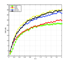
(a) SNR (fixed $s=10$)

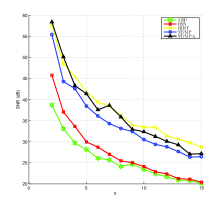
(b) SNR (fixed $m=1000$)

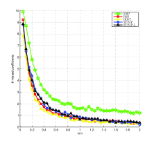
(c) number of missed coefficients

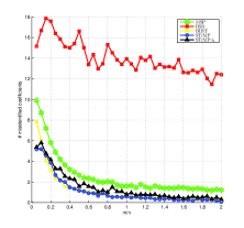
(d) number of misidentified coefficients

Figure 1: Accuracy experiments: Averaged SNR for (a) fixed $s=10$ and $n=1000$ while $m$ is changed with $m/n$ between $0.05$ and $2$, and (b) fixed $n=1000$ and $m=1000$ while $s$ is between 1 and 15. Averaged number of missed coefficients for (c) fixed $s=10$ and $n=1000$ with $m/n$ is between $0.05$ and $2$. Averaged number of misidentified coefficients for (d) $s=10$ and $n=1000$ with $m/n$ is between 0.05 and 2. STrMP, STrMP-$l_{1}$ and BIHT have similar performance, RSS and MSP perform similarly. And STrMP, STrMP-$l_{1}$ and BIHT are better than others.

In this experiment, we test the reconstruction accuracy in three different ways: the average signal-to-noise ratio (SNR), the average number of missed coefficients and the average number of misidentified coefficients, which are defined as follows

• SNR $:=10\log_{10}(\frac{\|x^{\sharp}\|^{2}}{\|x^{\sharp}-\hat{x}\|^{2}})$,

• Number of missed coefficients $:=|\{i\in[n]:\hat{x}_{i}\neq 0~{}\text{and}~{}x_{i}^{\sharp}=0\}|$,

• Number of misidentified coefficients $:=|\{i\in[n]:\hat{x}_{i}=0~{}\text{and}~{}x_{i}^{\sharp}\neq 0\}|$.

Here SNR is used to measure overall reconstruction performance of the recovery algorithms. Since the original signal $\hat{x}$ is sparse, it is also important to identify the support of original signal. To measure this kind of performance, it is helpful to calculate the number of missed coefficients and of misidentified coefficients.

The numerical results are depicted in Figure 1. In this experiment, as mentioned before, we set $n=1000$. In Figure 1(a), Figure 1(c) and Figure 1(d), we fix $s=10$ and change $m/n$ within the range $[0.05,2]$ with the step $0.05$. And hence $40$ different $m/n$ are considered. For each $m/n$, we perform $100$ trials and record the average value. In Figure 1(b), we fix $n=1000$ and $m=1000$ while $s$ is between $1$ and $15$. We also repeat the experiment $100$ times for each $s$ and plot the mean value. The plots in Figure 1 show that STrMP, STrMP-$l_{1}$ and BIHT perform similarly. The performance of STrMP-$l_{1}$ and BIHT is slightly better than STrMP in SNR. Figure 1(d) shows that RSS exhibits poorer performance for the number of misidentified coefficients which are also observed and analyzed in [10].

4.2 Consistency Test

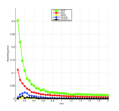
Figure 2: Consistency experiments: Averaged Hamming error between ${\rm sign}(Ax^{\sharp})$ and $y$ for $s=10$ with $m/n$ is between 0.05 and 2. As the figure depicts that STrMP and STrMP-$l_{1}$ have the similar performance as BIHT in terms of consistency test, and they are better than others.

In this subsection, we test whether $x^{\sharp}$ is consistence. To do that, we measure the Hamming error which is defined as follows:

• Hamming error $:=\|{\rm sign}(Ax^{\sharp})-y\|_{0}/m$.

For each $m/n$, we also perform 100 trials and record the average values. The plots in Figure 2 show that STrMP, STrMP-$l_{1}$ and BIHT work very well and they have better performance than that of MSP and RSS.

4.3 Speed Test

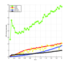
(a) CPU time (fixed $s=10$)

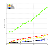
(b) CPU time (fixed $m=1000$)

Figure 3: Speed experiments: Averaged CPU time for (a) $s=10$ with $m/n$ is between 0.05 and 2, (b) $m=1000$ with $s$ is between 1 and 15. These demonstrate that STrMP and STrMP-$l_{1}$ take least time comparing with other algorithms.

At last, we test the speed of the algorithms by recoding the average computational time. Figure 3 depicts that STrMP and STrMP-$l_{1}$ outperform MSP significantly, and they are also faster than BIHT and RSS. The CPU time of MSP increases quickly as the measurements and the sparsity increase. However, time consuming of STrMP grows very slowly as measurements and sparsity increase, which is particularly striking for STrMP and STrMP-$l_{1}$. This is because the sub-problems of the STrMP algorithms are convex and unconstrained.

5 Conclusion

In this paper, we have introduced a fast and accurate greedy algorithm for the one-bit compressive sensing. The subproblem in STrMP is convex and unconstraint. And hence, STrMP algorithm is faster than previously existing one-bit compressed sensing algorithms. The choose of the first index plays an important role in STrMP. We prove that the first index belongs to the support of the original signal with high probability provided $m=O(s\log n)$. The numerical experiments show that the recovery performance of STrMP and STrMP-$l_{1}$ algorithm are similar with that of BIHT, and they are much better than that of RSS and MSP. One can note that the main part of STrMP is as concise as OMP. So, it will be very interesting to investigate the convergence property of STrMP using the technology developed in the study of OMP [14, 11, 19].

Appendix Appendix A Proofs of Theorems 1 and 2

Proof of Theorem 1.

To this end, we only need to prove that $x^{\sharp}$ satisfies

• consistence, i.e. ${\rm sign}(Ax^{\sharp})=y$,

• sparsity, i.e. $\|x^{\sharp}\|_{0}\leq\|{\hat{x}}\|_{0}$,

• normalization, i.e. $\|Ax^{\sharp}\|_{1}=c_{0}$.

We first consider

$${\rm sign}(Ax^{\sharp}) = {\rm sign}(A_{[n]\setminus\{j_{0}\}}z^{\sharp}+x_{j_{0}}^{\sharp}A_{j_{0}})$$

$$= {\rm sign}\left(\left(I-\frac{A_{j_{0}}y^{\top}}{y^{\top}A_{j_{0}}}\right)A_{[n]\setminus\{j_{0}\}}z^{\sharp}+\frac{c_{0}}{y^{\top}A_{j_{0}}}A_{j_{0}}\right)$$

$$= {\rm sign}(Pz^{\sharp}+q)=y,$$

which implies that (i). We turn to (iii). Note that

$$\|Ax^{\sharp}\|_{1} = y^{\top}Ax^{\sharp}=y^{\top}A_{[n]\setminus j_{0}}z^{\sharp}+y^{\top}A_{j_{0}}x^{\sharp}_{j_{0}}$$

$$= y^{\top}A_{[n]\setminus j_{0}}z^{\sharp}+y^{\top}A_{j_{0}}\frac{c_{0}-y^{\top}A_{[n]\setminus j_{0}}z^{\sharp}}{y^{\top}A_{j_{0}}}=c_{0}.$$

We arrive at (iii). We next consider (ii). To this end, we need to show that

$$\|x^{\sharp}\|_{0}\leq\|\hat{x}\|_{0}.$$

Without loss of generality, we can assume that $\|A\hat{x}\|_{1}=y^{\top}A\hat{x}=c_{0}$ (otherwise, we can multiply $\hat{x}$ by a positive constant ), which implies that

$$\hat{x}_{j_{0}}=\frac{c_{0}-y^{\top}A_{[n]\setminus\{j_{0}\}}\hat{x}_{[n]\setminus j_{0}}}{y^{\top}A_{j_{0}}}.$$ (10)

Then a simple calculation shows that

$$y = {\rm sign}(A{\hat{x}})={\rm sign}(A_{[n]\setminus j_{0}}{\hat{x}}_{[n]\setminus j_{0}}+A_{j_{0}}{\hat{x}}_{j_{0}})$$

$$= {\rm sign}(P\hat{x}_{[n]\setminus\{j_{0}\}}+q).$$

Here, in the last equality, we use (10). And hence $\hat{x}_{[n]\setminus\{j_{0}\}}$ satisfies the constraint condition (5) which implies that

$$\|z^{\sharp}\|_{0}\leq\|\hat{x}_{[n]\setminus\{j_{0}\}}\|_{0}=\|\hat{x}\|_{0}-1.$$

So, the definition of $x^{\sharp}$ implies that

$$\|x^{\sharp}\|_{0}\leq\|z^{\sharp}\|_{0}+1\leq\|\hat{x}\|_{0}.$$

We arrive at the conclusion. ∎

To prove Theorem 2, we first introduce Hoeffding-type inequality (see [15, Propsition 5.10]).

Lemma 1 (Hoeffding-type inequality):

Let $\zeta_{1},\ldots,\zeta_{n}$ be independent centered sub-gaussian random variables, and $K=\max\limits_{i}\|\zeta_{i}\|_{\psi_{2}}$. Then for every $a=(a_{1},\ldots,a_{n})\in\mathbb{R}^{n}$ and every $\epsilon\geq 0$, we have

$$P\{|\sum\limits_{i=1}^{n}a_{i}\zeta_{i}|\geq\epsilon\}\leq e\cdot\exp(-\frac{c_{1}\epsilon^{2}}{K^{2}\|a\|_{2}^{2}}),$$

where $c_{1}>0$ is an absolute constant.

Here, for a sub-gaussian random variable $\xi$,

$$\|\xi\|_{\psi_{2}}:=\mathop{\rm sup}\limits_{p\geq 1}({\mathbb{E}}\lvert\xi\rvert^{p})^{1/p}$$

(see also [15, Definition 5.7]). For a standard normal variable $\xi$, $\|\xi\|_{\psi_{2}}$ is bounded by $\sqrt{2}$. We are now turning to the proof of our theorem.

Proof of Theorem 2.

Without loss of generality, we can suppose that $\|\hat{x}\|_{2}=1$ and $\hat{x}_{\jmath}>0$ where $\jmath:=\mathop{\rm argmax}\limits_{i\in[n]}|\hat{x}_{i}|$. We claim that, for any $\epsilon>0$

$${\mathbb{P}}\{\max\limits_{k\notin{\rm supp}(\hat{x})}\lvert\langle{A_{k},y}\rangle\rvert<\sqrt{m\epsilon^{2}+2m\log(n-s)}\}\geq 1-\exp(-\frac{\epsilon^{2}}{2}),$$ (11)

and

$${\mathbb{P}}\{|\langle{A_{\jmath},y}\rangle|\geq 2\cdot m\frac{\hat{x}_{\jmath}}{\sqrt{2\pi}}-\epsilon\sqrt{m}\}\geq 1-e\cdot\exp(-\frac{c_{1}\epsilon^{2}}{8}).$$ (12)

Combining (11) and (12), to prove the conclusion we just need to show that

$$2\cdot m\frac{\hat{x}_{\jmath}}{\sqrt{2\pi}}-\epsilon\sqrt{m}\geq\sqrt{m\epsilon^{2}+2m\log(n-s)},$$ (13)

which is equivalent to

$$\sqrt{m}\cdot\frac{2\hat{x}_{\jmath}}{\sqrt{2\pi}}\geq\sqrt{\epsilon^{2}+2\log(n-s)}+\epsilon.$$ (14)

Indeed, note that $\hat{x}_{\jmath}=\|\hat{x}\|_{\infty}\geq\frac{1}{\sqrt{s}}$ with $\hat{x}$ being $s$-sparse, we have

$$\sqrt{m}\cdot\frac{2\hat{x}_{\jmath}}{\sqrt{2\pi}}\geq\sqrt{\frac{2}{{\pi}}}\cdot\sqrt{\frac{m}{s}}\geq\sqrt{\epsilon^{2}+2\log(n-s)}+\epsilon,$$

which implies (14) and hence (13) holds. Here, in the last inequality, we use

$$m\geq\frac{\pi}{2}s(\epsilon+\sqrt{\epsilon^{2}+2\log(n-s)})^{2}.$$ (15)

Hence, if the condition (15) is satisfied, we have

$$\mathop{\rm argmax}\limits_{i\in[n]}{|(A^{\top}{\rm sign}(A\hat{x}))_{i}|}\in{\rm supp}(\hat{x})$$

holds, with probability at least $1-2e\cdot\exp(-c\epsilon^{2})$, which implies the conclusion, where $c:=\min\{1,c_{1}/8\}$.

To this end, we still need to prove (11) and (12). We first consider (11). According to $y={\rm sign}(A\hat{x})$, we obtain that the entries of $y$ are $i.i.d.$ Bernoulli random variables, and they are independent of entries of $A_{k}$ for those $k\notin{\rm supp}(\hat{x})$. Note that $\langle{A_{k},y}\rangle\sim\mathcal{N}(0,m)$ provided $k\notin{\rm supp}(\hat{x})$. The Gaussian concentration inequality implies

$$P\{|\langle{A_{k},y}\rangle|<t\}\geq 1-\exp\left(-\frac{t^{2}}{2m}\right),$$

where $t>0$. Since $\hat{x}$ is $s$-sparse, there are $(n-s)$ entries do not belong to ${\rm supp}(\hat{x})$. By using the union bound, we have

$${\mathbb{P}}\{\max\limits_{k\notin{\rm supp}(\hat{x})}|\langle{A_{k},y}\rangle|<t\}\geq 1-(n-s)\exp\left(-\frac{t^{2}}{2m}\right).$$

Taking $t=\sqrt{m\epsilon^{2}+2m\log(n-s)}$, we obtain that

$${\mathbb{P}}\{\max\limits_{k\notin{\rm supp}(\hat{x})}|\langle{A_{k},y}\rangle|<\sqrt{m\epsilon^{2}+2m\log(n-s)}\}\geq 1-\exp\left(-\frac{\epsilon^{2}}{2}\right).$$

We next turn to (12). Without loss of generality we can assume that $\hat{x}_{\jmath}>0$. Note that $A_{i\jmath}y_{i},~{}i\in[m]$ are $i.i.d.$ random variables since $y_{i}$ only depends on the $i$th row of $A$. Then for every $\epsilon\geq 0$

$${\mathbb{P}}\{|A_{i\jmath}y_{i}|\geq\epsilon\}={\mathbb{P}}\{|A_{i\jmath}|\geq\epsilon\}\leq\exp(-\frac{\epsilon^{2}}{2}),$$

which implies that $A_{i\jmath}y_{i},~{}i\in[m]$ are $i.i.d.$ sub-gaussian random variables. We next calculate the expectation of $A_{i\jmath}y_{i}$. Let $\xi:=A_{i\jmath}$ and $\eta:=\sum\limits_{k\neq\jmath}A_{ik}\hat{x}_{k}$. Then $\xi\sim\mathcal{N}(0,1)$ and $\eta\sim\mathcal{N}(0,1-\hat{x}_{\jmath}^{2})$. Also, note that $\xi$ and $\eta$ are independent and

$${\mathbb{E}}(A_{i\jmath}y_{i})={\mathbb{E}}(A_{i\jmath}\cdot{\rm sign}(A_{i\jmath}\hat{x}_{\jmath}+\sum\limits_{k\neq\jmath}A_{ik}\hat{x}_{k}))={\mathbb{E}}(\xi\cdot{\rm sign}(\xi\hat{x}_{\jmath}+\eta)).$$

Now we have

$${\mathbb{E}}(A_{i\jmath}y_{i}) = \int_{-\infty}^{\infty}\int_{-\infty}^{\infty}\xi\cdot{\rm sign}(\xi\hat{x}_{\jmath}+\eta)\frac{1}{\sqrt{2\pi}}e^{-\frac{\xi^{2}}{2}}\frac{1}{\sqrt{2\pi(1-\hat{x}_{\jmath}^{2})}}e^{-\frac{\eta^{2}}{2(1-\hat{x}_{\jmath}^{2})}}\,\mathrm{d}\xi\,\mathrm{d}\eta$$ (16)

$$= \int_{-\infty}^{\infty}\int_{-\infty}^{-\frac{\eta}{\hat{x}_{\jmath}}}(-\xi)\frac{1}{\sqrt{2\pi}}e^{-\frac{\xi^{2}}{2}}\frac{1}{\sqrt{2\pi(1-\hat{x}_{\jmath}^{2})}}e^{-\frac{\eta^{2}}{2(1-\hat{x}_{\jmath}^{2})}}\,\mathrm{d}\xi\,\mathrm{d}\eta$$

$$+\>\int_{-\infty}^{\infty}\int_{-\frac{\eta}{\hat{x}_{\jmath}}}^{\infty}\xi\frac{1}{\sqrt{2\pi}}e^{-\frac{\xi^{2}}{2}}\frac{1}{\sqrt{2\pi(1-\hat{x}_{\jmath}^{2})}}e^{-\frac{\eta^{2}}{2(1-\hat{x}_{\jmath}^{2})}}\,\mathrm{d}\xi\,\mathrm{d}\eta$$

$$= 2\frac{\hat{x}_{\jmath}}{\sqrt{2\pi}}.$$ (17)

By using Lemma 1, we can get

$${\mathbb{P}}\{|\sum\limits_{i=1}^{m}(A_{i\jmath}y_{i}-{\mathbb{E}}(A_{i\jmath}y_{i}))|\geq\epsilon\sqrt{m}\}\leq e\cdot\exp(-{c_{1}\epsilon^{2}/8}),$$

where $c_{1}$ is an absolute constant. Then

$${\mathbb{P}}\{|\sum\limits_{i=1}^{m}A_{i\jmath}y_{i}|\geq m\cdot{\mathbb{E}}(A_{i\jmath}y_{i})-\epsilon\sqrt{m}\}\geq 1-e\cdot\exp(-c_{1}\epsilon^{2}/8).$$

∎

Remark 5.

We also make numerical experiments to test the success probability of the choose of the first index. We set $n=1000,s=15$ and change $m$ within the range $[30,200]$. We repeat the experiment $100$ times for each $m$ and calculate the success rate. The numerical results show that $m\thickapprox 150$ measurements are enough for correctly selecting the first index with the success rate being 1.

Appendix Appendix B Two-Point Step Size Gradient Method

The Step 6 of STrMP algorithms is to use the two-point step size gradient method [1]. We show it in Algorithm 2. The algorithm is usually to solve unconstrained optimization problems in the form of

$$\min_{x\in{{\mathbb{R}}}^{n}}f(x),$$ (18)

where $f(x)$ is derivable. For more details see [1].

Algorithm 2 Two-Point Step Size Gradient Method

0:  $0\leq\varepsilon\ll 1$ Initialization: $x_{1}\in{{\mathbb{R}}}^{n}$, $k:=1$

1:  while $\|\nabla f(x_{k})\|_{2}>\varepsilon$ do

2:     $d_{k}=-\nabla f(x_{k})$

3:     if $k=1$ then

4:        using exact line search or other methods to find first step $\alpha_{1}$.

5:     else

6:        $\alpha_{k}=s_{k-1}^{\top}y_{k-1}/\|y_{k-1}\|_{2}^{2}$, where

$$s_{k-1}=x_{k}-x_{k-1},~{}y_{k-1}=\nabla f(x_{k})-\nabla f(x_{k-1}).$$

7:     end if

8:     $x_{k+1}:=x_{k}+\alpha_{k}d_{k}$, $k:=k+1$

9:  end while

9:  $x_{k}$

References

- [1] Jonathan Barzilai and Jonathan M. Borwein. Two-point step size gradient methods. IMA Journal of Numerical Analysis, 8(1):141–148, 1988.
- [2] Thomas Blumensath and Mike E. Davies. Iterative hard thresholding for compressed sensing. Applied and Computational Harmonic Analysis, 27(3):265–274, 2009.
- [3] Petros T. Boufounos. Greedy sparse signal reconstruction from sign measurements. In Asilomar Conference on Signals, Systems and Computers, pages 1305–1309, 2009.
- [4] Petros T. Boufounos and Richard G. Baraniuk. 1-bit compressive sensing. In Proceedings of the 42nd Annual Conference on Information Sciences and Systems (CISS), pages 16–21, 2008.
- [5] Emmanuel J. Candès, Justin K. Romberg, and Terence Tao. Stable signal recovery from incomplete and inaccurate measurements. Communications on Pure and Applied Mathematics, 59(8):1207–1223, 2006.
- [6] Emmanuel J. Candès and Terence Tao. Decoding by linear programming. IEEE Transactions on Information Theory, 51(12):4203–4215, 2005.
- [7] Wei Dai, Olgica Milenkovic. Subspace pursuit for compressive sensing signal reconstruction, IEEE Transactions on Information Theory, 55(5): 2230-2249, 2009.
- [8] David L. Donoho. Compressed sensing. IEEE Transactions on Information Theory, 52(4):1289–1306, 2006.
- [9] Laurent Jacques, Jason N. Laska, Petros T. Boufounos, and Richard G. Baraniuk. Robust 1-bit compressive sensing via binary stable embeddings of sparse vectors. IEEE Transactions on Information Theory, 59(4):2082–2102, 2013.
- [10] Jason N. Laska, Zaiwen Wen, Wotao Yin, and Richard G. Baraniuk. Trust, but verify: Fast and accurate signal recovery from 1-bit compressive measurements. IEEE Transactions on Signal Processing, 59(11):5289–5301, 2011.
- [11] Deanna Needell, Joel A. Tropp. CoSaMP: Iterative signal recovery from incomplete and inaccurate samples. Applied and Computational Harmonic Analysis, 26(3): 301-321, 2009.
- [12] Deanna Needell, Roman Vershynin. Uniform uncertainty principle and signal recovery via regularized orthogonal matching pursuit. Foundations of Computational Mathematics, 9(3): 317-334, 2009.
- [13] Yaniv Plan and Roman Vershynin. One-bit compressed sensing by linear programming. Communications on Pure and Applied Mathematics, 66(8):1275–1297, 2013.
- [14] Joel A. Tropp. Greed is good: Algorithmic results for sparse approximation. IEEE Transactions on Information Theory, 50(10):2231-2242, 2004.
- [15] Roman Vershynin. Introduction to the non-asymptotic analysis of random matrices. In Yonina C. Eldar and Gitta Kutyniok, editors, Compressed Sensing: Theory and Applications, pages 210–268. Cambridge University Press, 2012.
- [16] Yang Wang and Zhiqiang Xu. The performance of PCM quantization under tight frames representations. SIAM Journal on Mathematical Analysis, 44(4):2802-2823, 2012.
- [17] Zhiqiang Xu. The performance of orthogonal multi-matching pursuit under RIP. Available at: http://arxiv.org/abs/1304.1969.
- [18] Ming Yan, Yi Yang, and Stanely Osher. Robust 1-bit compressive sensing using adaptive outlier pursuit. IEEE Transactions on Signal Processing, 60(7):3868–3875, 2012.
- [19] Tong Zhang. Sparse recovery with Orthogonal Mathching Pursuit under RIP. IEEE Transactions on Information Theory, 57(9):6215–6221, 2011.