Nonlinear modes and symmetries in linearly-coupled pairs of $\mathcal{PT}$-invariant dimers

Abstract

 

The subject of the work are pairs of linearly coupled $\mathcal{PT}$-symmetric dimers. Two different settings are introduced, namely, straight-coupled dimers, where each gain site is linearly coupled to one gain and one loss site, and cross-coupled dimers, with each gain site coupled to two lossy ones. The latter pair with equal coupling coefficients represents a $\mathcal{PT}$-hypersymmetric quadrimer. We find symmetric and antisymmetric solutions in these systems, chiefly in an analytical form, and explore the existence, stability and dynamical behavior of such solutions by means of numerical methods. We thus identify bifurcations occurring in the systems, including spontaneous symmetry breaking and saddle-center bifurcations. Simulations demonstrate that evolution of unstable branches typically leads to blowup. However, in some cases unstable modes rearrange into stable ones.

 

I Introduction

Recently, quantum systems and their classical wave counterparts featuring the $\mathcal{PT}$ (parity-time) symmetry, supported by the balance between spatially separated gain and loss terms, have drawn a great deal of attention, as reviewed in Refs. Bender_review ; special-issues ; review . In this context, the straightforward similarity between the Schrödinger equation in quantum mechanics and the paraxial propagation equation in optics has made it possible to propose Muga ; PT_periodic and demonstrate in experiments experiment that the $\mathcal{PT}$  symmetry can be implemented in terms of the optical-beam propagation in waveguides with appropriately placed and mutually balanced gain and loss.

The optical realizations of the $\mathcal{PT}$ symmetry make it natural to extend this concept to nonlinear settings Musslimani2008 . In particular, solitons can be supported by the combination of the Kerr nonlinearity and spatially periodic complex potentials, whose odd imaginary part accounts for the balanced gain and loss, thus accounting for the $\mathcal{PT}$  symmetry. A detailed analysis demonstrates the existence of stability regions for such $\mathcal{PT}$-symmetric solitons, both bright Yang and dark ones dark ; vortices , as well as for two-dimensional vortices vortices . Alternatively, one-dimensional dual ; Driben ; Barash ; dual2 and two-dimensional Burlak bright $\mathcal{PT}$-symmetric solitons, and their one-dimensional dark counterparts dark-coupler can be built as stable objects in dual-core couplers, with the balanced gain and loss placed in the different cores. Stable bright solitons were also predicted in $\mathcal{PT}$-symmetric settings with the second-harmonic-generating (quadratic) nonlinearity chi2 .

Another class of nonlinear $\mathcal{PT}$-symmetric systems is represented by a pair of discrete (delta-functional) gain and loss elements Stuttgart , or the gain-loss dipole, with the imaginary part of the potential represented by the $\delta^{\prime}$ function of the coordinate Bangkok , which are embedded into a continuous medium with the cubic nonlinearity. The model with the the gain-loss dipole admits a full family of exact analytical solutions for solitons pinned to the $\mathcal{PT}$ dipole.

Further, discrete solitons were predicted in various chains of linear discrete and circular circular coupled $\mathcal{PT}$-symmetric elements and, more generally, in networks of coupled $\mathcal{PT}$-symmetric oligomers (dimers, quadrimers, etc.) KPZ ; KPZ0 ; KPZ1 . Parallel to incorporating the usual Kerr nonlinearity into the conservative part of the $\mathcal{PT}$ system, its gain-loss-antisymmetric part can be made nonlinear too, by introducing mutually balanced cubic gain and loss terms AKKZ ; we . This can be done in the simplest way in the context of discrete systems, by embedding nonlinear cores into linear chains we . Effects of combined linear and nonlinear $\mathcal{PT}$ terms on the existence and stability of optical solitons were studied too combined .

Although $\mathcal{PT}$-symmetric models belong, generally speaking, to the class of dissipative systems, the fact that they give rise to continuous families of modes, which exist due to the balance between the separated gain and loss with equal strengths, makes them similar to conservative systems. The $\mathcal{PT}$-symmetry of the modes gets broken with the increase of the gain-loss coefficient. Above the critical value of this coefficient, the solution typically undergoes blowup pelin_recent , due to the onset of the imbalance between the linear gain and loss. On the other hand, in the presence of the nonlinear $\mathcal{PT}$-balanced gain and loss terms, the symmetry breaking of the solutions may lead to the formation of a self-trapped asymmetric mode, rather than the blowup we . However, in the latter case the modes exist as isolated attractors (rather than continuous families), like in generic nonlinear dissipative systems, i.e., the $\mathcal{PT}$ symmetry is broken in that case too.

The purpose of the present work is to introduce nonlinear systems with double symmetries, $\mathcal{PT}$ and spatial, and explore results of the interplay between these symmetries. The simplest example of such a setting, which we construct and analyze here, are bi-dimers, i.e., pairs of two linearly coupled $\mathcal{PT}$-symmetric dimers with the on-site cubic nonlinearity. Two types of this setting are possible, both considered below: straight- and cross-coupled ones, in which, respectively, the gain and loss elements of one dimer are coupled to their counterparts in the parallel one, or, alternatively, the two dimers are set anti-parallel to each other, the gain pole of one being coupled to its lossy counterpart in the other. In earlier works, similar configurations were considered either for equal couplings between all the sites KPZ1 , or for special cases (e.g., cross-coupled dimers for a special form of unequal couplings were touched upon in Ref. KPZ0 ). None of the earlier considered bi-dimer settings included the above-mentioned nonlinear $\mathcal{PT}$-symmetric gain/loss terms, which are a part of the models introduced in the present work.

The paper is organized as follows. In Section II, we formulate the models of the straight- and cross-coupled bi-dimers. We report partial analytical and systematic numerical results, varying the linear gain/loss parameter, $\gamma_{0}$, in the presence of the nonlinear gain and loss terms with coefficient $\gamma_{2}$, for varieties of stationary modes in the straight- and cross-coupled bi-dimers in Sections III and IV, respectively. In particular, the cross-coupled bi-dimer with the two linear-coupling constants equal to each other may be considered as a $\mathcal{PT}$-hypersymmetric quadrimer. The paper is concluded by Section V, which also puts forward directions for future studies.

II Formulation of the models

II.1 The straight-coupled bi-dimer

We introduce a system of two linearly coupled $\mathcal{PT}$-symmetric dipoles, each one represented by complex variables $\psi_{A,B}^{(1,2)}$, where subscripts $A$ and $B$ stand for the gain and loss sites, while superscripts $1$ and $2$ refer to the dipole’s number. Stationary states with frequency $\omega$ are looked for in the form of

$$~{}\psi_{A,B}^{(1,2)}(t)=e^{-i\omega t}\phi_{A,B}^{(1,2)}.$$ (1)

The bi-dimers with the straight and cross couplings between the gain and loss sites are schematically shown, in terms of variables $\phi_{A,B}^{(1,2)}$, in the left and right panels of Fig. 1.

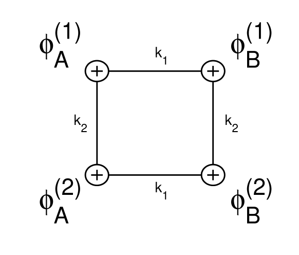
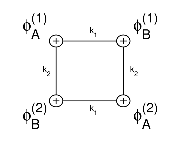
Figure 1: The left and right panels schematically display the straight- and cross-coupled bi-dimers, respectively.

Taking the dimer elements as defined in Ref. we (which includes the conservative cubic nonlinearity with real coefficient $\chi$), the straight-coupled bi-dimer is described by the following dynamical equations:

$$\begin{array}[]{l}{i\dot{\psi}_{A}^{(1)}=}\left({i\gamma_{0}-i\gamma_{2}}\left|{\psi_{A}^{(1)}}\right|{{}^{2}+\chi}\left|{\psi_{A}^{(1)}}\right|{{}^{2}}\right){\psi_{A}^{(1)}+k_{1}\psi_{B}^{(1)}+k_{2}\psi}_{A}^{(2)}{,}\\[9.0pt] {i\dot{\psi}_{B}^{(1)}=}\left({-i\gamma_{0}+i\gamma_{2}}\left|{\psi_{B}^{(1)}}\right|{{}^{2}+\chi}\left|{\psi_{B}^{(1)}}\right|{{}^{2}}\right){\psi_{B}^{(1)}+k_{1}\psi_{A}^{(1)}{+k_{2}\psi}_{B}^{(2)},}\end{array}$$ (2)

$$\begin{array}[]{l}{i\dot{\psi}_{A}^{(2)}=}\left({i\gamma_{0}-i\gamma_{2}}\left|{\psi_{A}^{(2)}}\right|{{}^{2}+\chi}\left|{\psi_{A}^{(2)}}\right|{{}^{2}}\right){\psi_{A}^{(2)}+k_{1}\psi_{B}^{(2)}+k_{2}\psi}_{A}^{(1)}{,}\\[9.0pt] {i\dot{\psi}_{B}^{(2)}=}\left({-i\gamma_{0}+i\gamma_{2}}\left|{\psi_{B}^{(2)}}\right|{{}^{2}+\chi}\left|{\psi_{B}^{(2)}}\right|{{}^{2}}\right){\psi_{B}^{(2)}+k_{1}\psi_{A}^{(2)}{+k_{2}\psi}_{B}^{(1)},}\end{array}$$ (3)

where $\gamma_{0}>0$ and $\gamma_{2}>0$ are the linear and nonlinear gain-loss coefficient, $k_{1}$ accounts for the linear coupling, inside a give dimer, between the sites at which the gain and loss are applied, and $k_{2}$ is a coefficient of the coupling between the parallel dimers. Then, stationary solutions are looked as per Eq. (1) with constant amplitudes $\phi_{A,B}^{(1,2)}$ satisfying a system of algebraic equations:

$$\begin{array}[]{l}{\omega\phi_{A}^{(1)}=}\left({i\gamma_{0}-i\gamma_{2}}\left|{\phi_{A}^{(1)}}\right|{{}^{2}+\chi}\left|{\phi_{A}^{(1)}}\right|{{}^{2}}\right){\phi_{A}^{(1)}+k_{1}\phi_{B}^{(1)}+k_{2}{\phi}_{A}^{(2)},}\\[9.0pt] {\omega\phi_{B}^{(1)}=}\left({-i\gamma_{0}+i\gamma_{2}}\left|{\phi_{B}^{(1)}}\right|{{}^{2}+\chi}\left|{\phi_{B}^{(1)}}\right|{{}^{2}}\right){\phi_{B}^{(1)}+k_{1}\phi_{A}^{(1)}{+k_{2}\phi}_{B}^{(2)},}\end{array}$$ (4)

$$\begin{array}[]{l}{\omega\phi_{A}^{(2)}=}\left({i\gamma_{0}-i\gamma_{2}}\left|{\phi_{A}^{(2)}}\right|{{}^{2}+\chi}\left|{\phi_{A}^{(2)}}\right|{{}^{2}}\right){\phi_{A}^{(2)}+k_{1}\phi_{B}^{(2)}+k_{2}{\phi}_{A}^{(1)},}\\[9.0pt] {\omega\phi_{B}^{(2)}=}\left({-i\gamma_{0}+i\gamma_{2}}\left|{\phi_{B}^{(2)}}\right|{{}^{2}+\chi}\left|{\phi_{B}^{(2)}}\right|{{}^{2}}\right){\phi_{B}^{(2)}+k_{1}\phi_{A}^{(2)}{+k_{2}\phi}_{B}^{(1)}.}\end{array}$$ (5)

Notice that in this model each site with linear gain features nonlinear loss and vice versa, as such a setting is likely to produce stable states we .

II.2 The cross-coupled bi-dimer

The system of two antiparallel linearly (cross-) coupled dimers is described by the following dynamical and static equations, cf. Eqs. (2)-(5):

$$\begin{array}[]{l}{i\dot{\psi}_{A}^{(1)}=}\left({i\gamma_{0}-i\gamma_{2}}\left|{\psi_{A}^{(1)}}\right|{{}^{2}+\chi}\left|{\psi_{A}^{(1)}}\right|{{}^{2}}\right){\psi_{A}^{(1)}+k_{1}\psi_{B}^{(1)}+k_{2}\psi}_{B}^{(2)}{,}\\[9.0pt] {i\dot{\psi}_{B}^{(1)}=}\left({-i\gamma_{0}+i\gamma_{2}}\left|{\psi_{B}^{(1)}}\right|{{}^{2}+\chi}\left|{\psi_{B}^{(1)}}\right|{{}^{2}}\right){\psi_{B}^{(1)}+k_{1}\psi_{A}^{(1)}{+k_{2}\psi}_{A}^{(2)},}\end{array}$$ (6)

$$\begin{array}[]{l}{i\dot{\psi}_{A}^{(2)}=}\left({i\gamma_{0}-i\gamma_{2}}\left|{\psi_{A}^{(2)}}\right|{{}^{2}+\chi}\left|{\psi_{A}^{(2)}}\right|{{}^{2}}\right){\psi_{A}^{(2)}+k_{1}\psi_{B}^{(2)}+k_{2}\psi}_{B}^{(1)}{,}\\[9.0pt] {i\dot{\psi}_{B}^{(2)}=}\left({-i\gamma_{0}+i\gamma_{2}}\left|{\psi_{B}^{(2)}}\right|{{}^{2}+\chi}\left|{\psi_{B}^{(2)}}\right|{{}^{2}}\right){\psi_{B}^{(2)}+k_{1}\psi_{A}^{(2)}{+k_{2}\psi}_{A}^{(1)},}\end{array}$$ (7)

$$\begin{array}[]{l}{\omega\phi_{A}^{(1)}=}\left({i\gamma_{0}-i\gamma_{2}}\left|{\phi_{A}^{(1)}}\right|{{}^{2}+\chi}\left|{\phi_{A}^{(1)}}\right|{{}^{2}}\right){\phi_{A}^{(1)}+k_{1}\phi_{B}^{(1)}+k_{2}{\phi}_{B}^{(2)},}\\[9.0pt] {\omega\phi_{B}^{(1)}=}\left({-i\gamma_{0}+i\gamma_{2}}\left|{\phi_{B}^{(1)}}\right|{{}^{2}+\chi}\left|{\phi_{B}^{(1)}}\right|{{}^{2}}\right){\phi_{B}^{(1)}+k_{1}\phi_{A}^{(1)}{+k_{2}\phi}_{A}^{(2)},}\end{array}$$ (8)

$$\begin{array}[]{l}{\omega\phi_{A}^{(2)}=}\left({i\gamma_{0}-i\gamma_{2}}\left|{\phi_{A}^{(2)}}\right|{{}^{2}+\chi}\left|{\phi_{A}^{(2)}}\right|{{}^{2}}\right){\phi_{A}^{(2)}+k_{1}\phi_{B}^{(2)}+k_{2}{\phi}_{B}^{(1)},}\\[9.0pt] {\omega\phi_{B}^{(2)}=}\left({-i\gamma_{0}+i\gamma_{2}}\left|{\phi_{B}^{(2)}}\right|{{}^{2}+\chi}\left|{\phi_{B}^{(2)}}\right|{{}^{2}}\right){\phi_{B}^{(2)}+k_{1}\phi_{A}^{(2)}{+k_{2}\phi}_{A}^{(1)}.}\end{array}$$ (9)

Here $k_{2}$ is again a real coupling constant. As said above, in the cross-coupled bi-dimers, each site with a linear gain is coupled to two sites with linear loss (and vice-versa). In particular, the case of the $\mathcal{PT}$ hypersymmetry (alias double symmetry) corresponds to $k_{2}=k_{1}$ (in the continuous model of the $\mathcal{PT}$-symmetric coupler, the extended symmetry of the same type was introduced in Refs. dual and Driben , under the name of “supersymmetry”, which we do not use here, to avoid confusion with the well-known supersymmetry between bosons and fermions in the quantum field theory). In the latter case, the cross-coupled bi-dimer may also be naturally called a $\mathcal{PT}$-hypersymmetric quadrupole.

In the particular case of $\chi=0$ and $\omega=0$, solutions to the hypersymmetric version of Eqs. (8) and (9) may be sought for in the form similar to that in the case of the single dimer we , viz.,

$$\phi_{A}^{(1,2)}=A_{1,2},~{}\phi_{B}^{(1,2)}=iB_{1,2},$$ (10)

where real amplitudes $A_{1,2}$ and $B_{1,2}$ obey the following system of four equations:

$$\left(\gamma_{0}-\gamma_{2}A_{1}^{2}\right)A_{1} = \left(\gamma_{0}-\gamma_{2}A_{2}^{2}\right)A_{2}=-k_{1}\left(B_{1}+B_{2}\right),$$

$$\left(\gamma_{0}-\gamma_{2}B_{1}^{2}\right)B_{1} = \left(\gamma_{0}-\gamma_{2}B_{2}^{2}\right)B_{2}=-k_{1}\left(A_{1}+A_{2}\right).$$ (11)

In particular, a corollary of Eqs. (11) is the following relations between the amplitudes:

$$A_{1}^{2}+A_{2}^{2}+A_{1}A_{2}=B_{1}^{2}+B_{2}^{2}+B_{1}B_{2}=\gamma_{0}/\gamma_{2}.$$ (12)

Below, we address the existence, stability and dynamics of nonlinear modes in both the straight- and cross-coupled bi-dimers.

III Straight-coupled bi-dimers

In this section, we first analytically seek for stationary solutions with (real) frequency $\omega$, as per Eqs. (4)-(5). Then, we will numerically explore the linear stability and nonlinear dynamics of these solutions.

III.1 Solutions for stationary modes

Using the amplitude-phase parametrization for the complex variables,

$$\phi_{A}^{(1)}=Ae^{i\theta_{1}},\ \phi_{B}^{(1)}=Be^{i\theta_{2}},\ \phi_{A}^{(2)}=Ce^{i\theta_{3}},\phi_{B}^{(2)}=De^{i\theta_{4}},$$ (13)

we have found nine branches of solutions to stationary equations (4) and (5), in both analytical and numerical forms, which are listed below.

1. Two solutions, which correspond to signs $\pm$ in the expression for $A^{2}$ in Eq. (14), with the unbroken spatial antisymmetry  and unbroken $\mathcal{PT}$ symmetry: $\phi_{A}^{(1)}=-\ \phi_{A}^{(2)}$, $\phi_{B}^{(1)}=-\phi_{B}^{(2)}$, $\left|\phi_{A}^{(1,2)}\right|^{2}=\left|\phi_{B}^{(1,2)}\right|^{2}$:

   $$A=B=C=D,$$

   $$\theta_{1}-\theta_{3}=\theta_{2}-\theta_{4}=\pi,$$

   $$A^{2}=\frac{\gamma_{0}\gamma_{2}+\chi(k_{2}+\omega)\pm\sqrt{k_{1}^{2}(\gamma_{2}^{2}+\chi^{2})-(\gamma_{0}\chi-\gamma_{2}(k_{2}+\omega))^{2}}}{\gamma_{2}^{2}+\chi^{2}}~{},$$

   $$\sin(\theta_{1}-\theta_{2})=\frac{\gamma_{0}-\gamma_{2}A^{2}}{k_{1}},$$

   $$\cos(\theta_{1}-\theta_{2})=\frac{k_{2}+\omega-\chi A^{2}}{k_{1}},$$ (14)

   Note that this solution satisfies the self-consistency condition, $\sin^{2}(\theta_{1}-\theta_{2})+\cos^{2}(\theta_{1}-\theta_{2})\equiv 1$. Of course, here and below only the solutions with $A^{2}>0$ are meaningful ones.

2. Two solutions with unbroken spatial symmetry and broken $\mathcal{PT}$ symmetry: $\phi_{A}^{(1)}=\ \phi_{A}^{(2)}$, $\phi_{B}^{(1)}=\phi_{B}^{(2)}$, $\left|\phi_{A}^{(1,2)}\right|^{2}\neq\left|\phi_{B}^{(1,2)}\right|^{2}$. These solution branches are non-generic (of codimension $1$), existing under a special condition,

   $$\chi\gamma_{0}=(k_{2}-\omega)\gamma_{2}.$$ (15)

   If this condition holds, the two analytical solutions are

   $$A=C,\ B=D,\ A^{2}+B^{2}=\frac{\gamma_{0}}{\gamma_{2}},$$

   $$A^{2}=\frac{\gamma_{0}\left(\gamma_{2}^{2}+\chi^{2}\right)\pm\sqrt{\left(\gamma_{2}^{2}+\chi^{2}\right)\left(-4k_{1}^{2}\gamma_{2}^{2}+\gamma_{0}^{2}\left(\gamma_{2}^{2}+\chi^{2}\right)\right)}}{2\gamma_{2}\left(\gamma_{2}^{2}+\chi^{2}\right)},$$

   $$\sin(\theta_{1}-\theta_{2})=\frac{(\gamma_{0}-\gamma_{2}A^{2})A}{k_{1}B},$$

   $$\cos(\theta_{1}-\theta_{2})=\frac{(\omega-k_{2}-\chi A^{2})A}{k_{1}B}.$$ (16)

   Further, the point of the spontaneous breakup of the spatial symmetry of solution (16), which should lead to fully asymmetric modes, can be found by looking for perturbed stationary solutions, $\phi_{A}^{(1,2)}=A\pm\delta\phi_{A}$, $\phi_{B}^{(1,2)}=iB\pm\delta\phi_{B}$, with infinitesimally small $\delta\phi_{A,B}$ . The substitution of this into Eqs. (4), (5) and the linearization with respect to the perturbations leads to a system of linear homogeneous equations,

   $$\left(2k_{2}-i\gamma_{0}+2i\gamma_{2}A^{2}\right)\delta\phi_{A}+i\gamma_{2}A^{2}\delta\phi_{A}^{\ast}-k_{1}\delta\phi_{B} = 0,$$

   $$\left(2k_{2}+i\gamma_{0}-2i\gamma_{2}B^{2}\right)\delta\phi_{A}+i\gamma_{2}B^{2}\delta\phi_{B}^{\ast}-k_{1}\delta\phi_{A} = 0.$$ (17)

   Splitting the complex perturbations into real and imaginary parts, $\delta\phi_{A,B}\equiv\delta\phi_{A,B}^{\prime}+i\delta\phi_{A,B}^{\prime\prime},$ transforms Eqs. (17) into a system of four equations, whose solvability condition yields an equation which determines the aforementioned point of the spontaneous symmetry breaking:

   $$\left|\begin{array}[]{cccc}2k_{2}&\gamma_{0}-\gamma_{2}A^{2}&-k_{1}&0\\ -\gamma_{0}+3\gamma_{2}A^{2}&2k_{2}&0&-k_{1}\\ -k_{1}&0&2k_{2}&2\gamma_{0}-3\gamma_{2}A^{2}\\ 0&-k_{1}&\gamma_{2}A^{2}&2k_{2}\end{array}\right|=0.$$ (18)

   The value of $k_{2}$ at which the symmetry breaking occurs can be found from Eq. (18) in an analytical form:

   $$k_{2}=\frac{1}{8}\left(2k_{1}^{2}-\gamma_{0}^{2}+6A^{2}\gamma_{0}\gamma_{2}-6A^{4}\gamma_{2}^{2}\right.$$ (19)

   $$\left.\pm\sqrt{-12k_{1}^{2}\gamma_{0}^{2}+\gamma_{0}^{4}+64A^{2}k_{1}^{2}\gamma_{0}\gamma_{2}-4A^{2}\gamma_{0}^{3}\gamma_{2}-64A^{4}k_{1}^{2}\gamma_{2}^{2}+4A^{4}\gamma_{0}^{2}\gamma_{2}^{2}}\right).$$ (20)

3. Two solutions with the unbroken spatial $\mathcal{PT}$ symmetries, $\phi_{A}^{(1)}=\ \phi_{A}^{(2)}$, $\phi_{B}^{(1)}=\phi_{B}^{(2)}$, $\left|\phi_{A}^{(1,2)}\right|^{2}=\left|\phi_{B}^{(1,2)}\right|^{2}$:

   $$A^{2}=B^{2}=C^{2}=D^{2}=\frac{\gamma_{0}\gamma_{2}+\chi(\omega-k_{2})\pm\sqrt{k_{1}^{2}(\gamma_{2}^{2}+\chi^{2})-(\gamma_{0}\chi+\gamma_{2}(k_{2}-\omega))^{2}}}{\gamma_{2}^{2}+\chi^{2}},$$

   $$\sin(\theta_{1}-\theta_{2})=\frac{\gamma_{0}-\gamma_{2}A^{2}}{k_{1}},$$

   $$\cos(\theta_{1}-\theta_{2})=\frac{\omega-k_{2}-\chi A^{2}}{k_{1}}.$$ (21)

4. Three solution branches with the broken spatial symmetry and unbroken $\mathcal{PT}$ symmetry, i.e., $A=B\neq C=D$, can be found only in a numerical form. Their profiles are shown in Fig. 5.

III.2 Stability of the stationary modes

Since the solution branches given by Eq. (16) exist only under condition (15), for being able to compare them with other solutions, we fix the coefficients as $\gamma_{2}=1,\ k_{1}=1,\ k_{2}=\omega=0.1$, and $\chi=0$, unless stated otherwise, while the main control parameter, the linear gain-loss coefficient, $\gamma_{0}$, is subject to variation. Note that, according to Eqs. (2)-(3), at $\chi=0$ coefficient $\gamma_{2}$ affects solely the absolute values of the solutions, but not their phases (actually, it does not significantly affect the stability of the solutions either). For this reason, $\gamma_{2}=1$ is fixed here, without the loss of generality.

Figures 2-6 present properties of the straight-coupled bi-dimers of the types enumerated above. The stability of the solutions was identified via numerical computation of eigenvalues, $\lambda$, for modes of small perturbations determined by the linearized version of Eqs. (2)-(3), which is produced by the substitution of the expression for perturbed solutions,

$$\psi_{A,B}^{(1,2)}=e^{-i\omega t}\left\{\psi_{A,B,\mathrm{eq}}^{(1,2)}+\delta\left[a_{A,B}^{(1,2)}e^{\lambda t}+\left(b_{A,B}^{(1,2)}\right)^{\star}e^{\lambda^{\star}t}\right]\right\},$$ (22)

into Eqs. (2)-(3), and subsequent linearization with respect to the infinitesimal amplitude, $\delta$. The instability is implied by the existence of a positive real part of any eigenvalue, $\lambda\equiv\lambda_{r}+i\lambda_{i}$, with $\lambda_{r}>0$.

Figure 2 represents the solution branches defined by Eq. (14), with thick red and thin blue curves corresponding to the upper and lower signs in the expression for $A^{2}$, respectively. The thin blue branch starts at $\gamma_{0}=0.98$, and is stable until $\gamma_{0}=1.76$, where two pairs of purely imaginary eigenvalues collide and create a complex quartet, thus causing the destabilization of the underlying stationary solution through an oscillatory instability. An additional instability arises at $\gamma_{0}=2$, through the bifurcation of an imaginary eigenvalue pair into a real one. The thick red branch exists and is unstable for all values of $\gamma_{0}$. The respective instability is accounted for by two pairs of real eigenvalues that are too close to be distinguished in Figure 2, coexisting with a pair of purely imaginary ones.

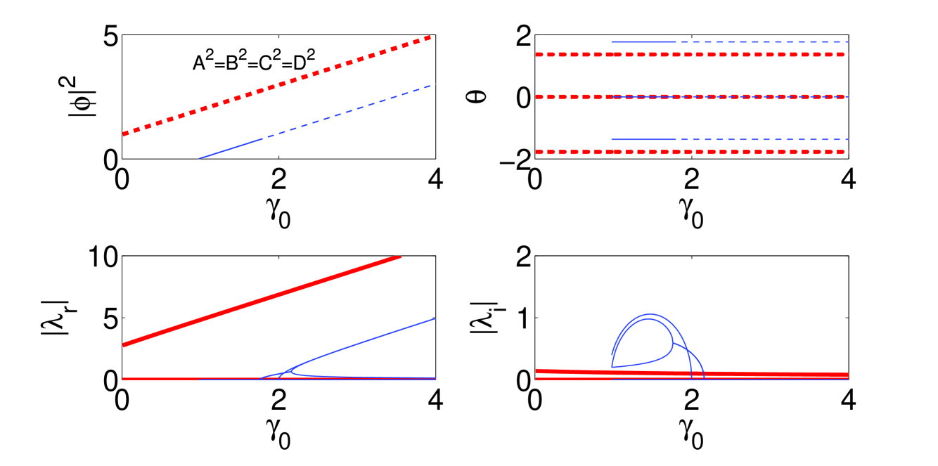
Figure 2: (Color online) Solutions for the straight-coupled bi-dimers, given by Eq. (14), for fixed parameters $\gamma_{2}=1,\ k_{2}=0.1,\ \chi=0,\ k_{1}=1$, and $\omega=0.1$. Stable and unstable portions of the solution families are plotted by solid and dashed lines, respectively. The thick red and thin blue line branches correspond, respectively, to “$+$” and “$-$” signs in the expression for $A^{2}$ in Eq. (14). The four panels show the squared absolute values (top left), phases (top right), as well as real ($\lambda_{r}$, bottom left) and imaginary ($\lambda_{i}$, bottom right) parts of the linear stability eigenvalues for the two branches.

Next, the solutions given by Eqs. (16) and (21) are shown in Figs. 3 and 4, respectively. The black (shown in Fig. 4) and magenta (the asymmetric branch in Fig. 3) solution branches correspond, respectively, to the upper and lower signs in the expression for $A^{2}$ in Eq. (16), while the thickest red and thinnest blue curves represent solutions (21) with the upper and lower signs, respectively. The thinnest blue branch starts at $\gamma_{0}=1$ and quickly becomes unstable at $\gamma_{0}=1.02$ due to a pair of real eigenvalues that arise from zero. The magenta and black branches bifurcate from the thinnest blue one at $\gamma_{0}=2$, implying the onset of the $\mathcal{PT}$-symmetry breaking at this point. The magenta branch is always unstable, while its black counterpart is unstable at $\gamma_{0}<2.82$, and stable at $\gamma_{0}>2.82$. It is important here to stress that, while for the thinnest blue and thickest red branches $\omega$ is fixed in the course of the continuation in $\gamma_{0}$, this is not the case for the black and magenta branches. In particular, condition (15) fully determines $\omega$ for a given set of other parameters. So, similarly to what is known from the earlier works we ; duanmu , such non-generic branches exist at isolated values of parameters, such as the frequency (once all other parameters of the system are fixed).

Figure 3: (Color online) Profiles of the straight-coupled bi-dimer solutions given by Eq. (16) (magenta curves) and Eq. (21) (thin blue and thick red ones), for fixed parameters $\gamma_{2}=1,\ \omega=k_{2}=0.1,\ \chi=0$ and $k_{1}=1$. The thinnest blue and thickest red branches correspond to “$-$” and “$+$” signs in the expression for the amplitude in Eq. (21), respectively. The magenta branches with the intermediate thickness correspond to the “$-$” sign in the expression for $A^{2}$ in Eq. (16), while the curve corresponding to the “$+$” sign is plotted in Fig. 4.

Figure 4: (Color online) Profiles of the straight-coupled bi-dimer solution corresponding to the “$+$” sign in Eq. (16), for fixed parameters $\gamma_{2}=1,\ \omega=k_{2}=0.1,\ \chi=0$ and $k_{1}=1$.

We have also found three solution branches with $A=B$ and $C=D$ numerically, which are shown in Fig. 5. A bifurcation point is in this case located at $\gamma_{0}=1.56$, when two solution branches, represented by the thinnest blue and the thinner red lines, arise from a saddle-center bifurcation. However, both these branches are unstable, bearing at least one real pair of eigenvalues (the one represented by the blue line acquires a second instability pair at $\gamma_{0}=2.26$, while the branch corresponding to the thinner red line always possesses at least two pairs with positive real parts). The thickest black branch exists and is unstable for all $\gamma_{0}$ too (again, with one real pair for all values of $\gamma_{0}$, and an additional one emerging from the bifurcation of an imaginary pair into a real one at $\gamma_{0}=1.74$). The difference in the values of amplitudes $A\equiv B$ between all the three branches is very small, but the difference in the values of $C\equiv D$ between the branches may be significant, especially for the thinner red branch, whose $C\equiv D$ amplitudes are approaching zero as the gain/loss parameter $\gamma_{0}$ increases.

Figure 5: (Color online) Profiles of the straight-coupled bi-dimer solutions with $A=B$ and $C=D$. Note that the phases are not constant, even if they seem to be nearly constant, except for $\theta_{1}\equiv 0$. For a detailed description of the relevant branches see the text.

Some case examples of the dynamical behavior of these nine branches of the solutions are shown in Fig. 6. Among the nine above-mentioned branches, only three feature stable dynamics in certain intervals of $\gamma_{0}$, viz., the thin blue branch in Fig. 2 for $0.98\leq\gamma_{0}\leq 1.76$, the thinnest blue branch in Fig. 3 for $1\leq\gamma_{0}\leq 1.01$, and the black one in Fig. 4 for $\gamma_{0}\geq 2.82$. The perturbed evolution of modes belonging to unstable branches always demonstrate an indefinite growth of the amplitude (blowup) at the site where the gain is applied, in the examples that we have considered. Amplitudes at the loss sites decay very slowly in the solutions represented by the the thin blue branch, whereas they grow in the solutions corresponding to the thick red branch, though very slowly, too.

(a)  thin blue branch

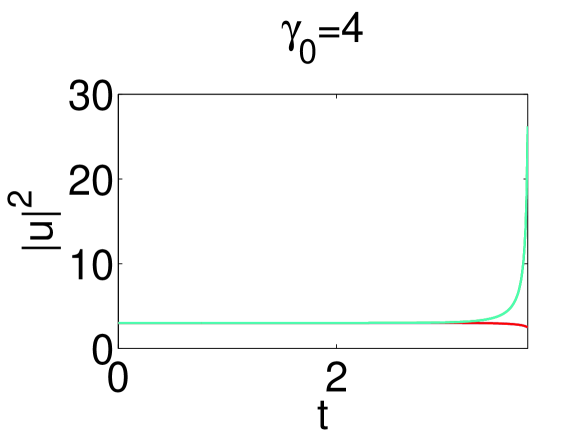
(b)  thin blue branch

(c)  thick red branch

Figure 6: (Color online) The evolution of the straight-coupled modes from Fig. 2. Here and in dynamical simulations displayed below, the simulations were performed with random initial perturbations of relative size $\sim 10^{-5}$ added to the stationary solutions. Panel a) shows the stable dynamics of the solutions represented by the thin blue branch at $\gamma_{0}=1.5$. Panels b) and c) show the instability of both thin blue and thick red branches at $\gamma_{0}=4$, where $B\equiv D$ grows exponentially, while $A\equiv C$ eventually decays in b) but grows in c).

IV Cross-coupled bi-dimers

Similarly to the previous section, we here start by seeking for stationary solutions with frequency $\omega$, as per Eqs. (8) and (9). Subsequently, we explore the linear stability and nonlinear dynamics of such solutions.

IV.1 Solutions for stationary modes

The cross-coupled bi-dimer complexes possess all the solutions that an ordinary nonlinear dimer possesses (see for relevant details the recent work duanmu ). This can be immediately seen by setting $\phi_{A}^{(1)}=\phi_{A}^{(2)},\phi_{B}^{(1)}=\phi_{B}^{(2)}$, which reduces Eqs. (8) and (9) to an ordinary dimer.

Besides those obvious solutions, we have not been able to obtain other stationary modes for cross-coupled bi-dimers in a general analytical form. Only two branches of solutions are found in this case, without any symmetry-breaking point, as shown in Fig. 7. However, it cannot be ruled out that additional branches, potentially featuring a symmetry breaking, may exist in this setting.

The branch with equal absolute values of the amplitudes at all four sites (the red one in Fig. 7), i.e., with $A=B=C=D$ (in other words, it is a hypersymmetric quadrimer, as it is defined above), is one that can be found in an explicit analytical form:

$$A=B=C=D,$$

$$\phi_{1}=\phi_{3},\ \phi_{2}=\phi_{4},$$

$$\sin(\phi_{2}-\phi_{1})=\frac{\gamma_{2}A^{2}-\gamma_{0}}{k_{1}+k_{2}},$$

$$\cos(\phi_{2}-\phi_{1})=\frac{\omega-E}{k_{1}+k_{2}}.$$ (23)

The other numerically identified solution branch is shown by the blue line in Fig. 7. It is characterized by relations $A=B,\ C=D$, i.e., it features the broken spatial symmetry and unbroken $\mathcal{PT}$ symmetry, according to Eq. (13).

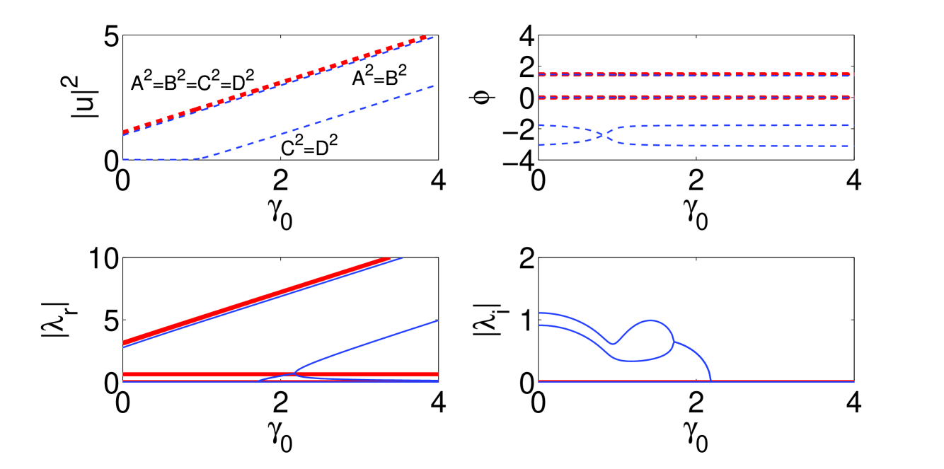
Figure 7: (Color online) Solution profiles for the cross-coupled bi-dimers at fixed parameters $\gamma_{2}=1,\ \omega=k_{2}=0.1,\ \chi=0$, and $\ k_{1}=1$. The thin blue and thick red lines pertain, respectively, to the numerically found solution and the analytical one given by Eq. (23), respectively.

IV.2 Stability of the stationary modes

Both solution branches (red and blue ones) for the cross-coupled bi-dimers, which are plotted in Fig. 7, turn out to be unstable. The thick red branch, which represents the analytically found solution, always has two pairs of real eigenvalues. One of them is approximately constant, while the other grows continuously. For the thin blue branch, there is always one pair of real eigenvalues that grows indefinitely too. On the other hand, there are two pairs of imaginary eigenvalues that collide, giving rise to a complex quartet, and the respective oscillatory instability, at $\gamma_{0}=1.72$. Then they collide again at $\gamma_{0}=2.19$, turning into two pairs of real eigenvalues.

The perturbed evolution of these unstable branches is shown in Fig. 8. The evolution of the solutions corresponding to the thin blue branch is similar to the examples discussed above for the straightly-coupled bi-dimer, leading to the blowup (indefinite growth). However, it is worthy to note that, unlike the other unstable branches, which were considered above, whose amplitudes blow up due to the instability, the evolution of solutions associated with the thick red branch is quite different. It leads at first to a breakup of the $\mathcal{PT}$ symmetry, bringing the pair of amplitudes, $B=D$, very close to zero. Subsequently, the instability results in establishment of a stable mode with squared absolute values of the amplitudes $A^{2}=C^{2}=3.67$ and $B^{2}=D^{2}=0.33$ (i.e., still with the broken $\mathcal{PT}$ symmetry), and phases locked to $\theta_{1}=\theta_{3},\ \theta_{2}=\theta_{4}$ and $\theta_{1}-\theta_{2}=\pi/2$. In fact, this eventually established solution can be identified as a stable state of a the usual (single) nonlinear dimer, which was named “case II” in Ref. duanmu .

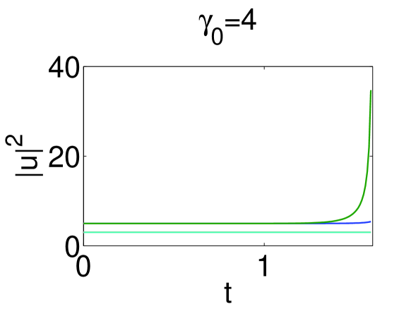
(a)  thin blue branch

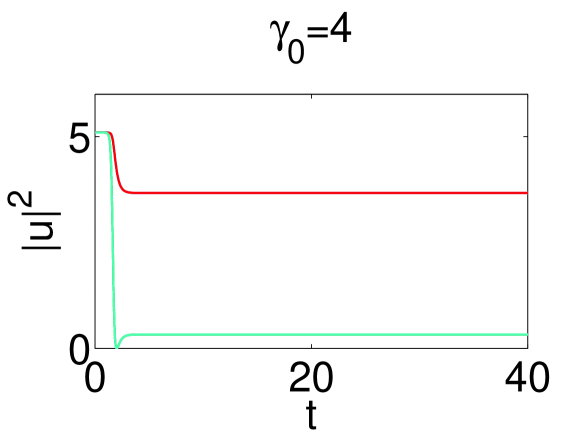
(b)  thick red branch

Figure 8: (Color online) Perturbed evolution of the solutions for the cross-coupled bi-dimers corresponding to Fig. 7.

V Conclusion

We have introduced two settings bearing both linear and nonlinear gain and loss, which implement, in the simplest form, different fundamental types of symmetries for $\mathcal{PT}$-invariant systems. Both settings are built of two linearly coupled intrinsically nonlinear $\mathcal{PT}$-symmetric dipoles (which, by themselves, provide for the simplest implementations of the $\mathcal{PT}$ invariance). One of the configurations is arranged as a straight-coupled bi-dimer, with each linear-gain site linearly-coupled to another linear-gain one, and a linear-loss site. The second configuration is the cross-coupled bi-dimer, with each of the gain sites coupled to two lossy ones. The latter system may also implement a $\mathcal{PT}$-hypersymmetric quadrimer, in the case when all the linear-coupling coefficients are equal.

For these two systems, we have identified a number of solutions analytically, including those keeping both the spatial and the $\mathcal{PT}$-symmetries unbroken, as well as solutions that break one of these symmetries. These solutions present a number of noteworthy features, in terms of the bifurcation theory. In particular, symmetry-breaking and saddle-center bifurcations were found in these settings. Instabilities typically lead to blowup of the solutions, but examples of convergence to another attractor were also identified.

These fundamental systems may be used as building blocks to construct lattices consisting of either straight- or cross-coupled bi-dimers, which should be a natural next step of the analysis. It would also be of particular interest to extend considerations to a three-dimensional $\mathcal{PT}$-symmetric system, i.e., to explore $\mathcal{PT}$-symmetric cubes and configurations which may be developed from them. Studies along these directions are currently in progress.